Planar Domain Indices: A Method for Measuring a Quality of a Single Component in. Two-component Pixels. T. R. Clarke. 1. , M. S. Moran. 2. , E. M. Barnes. 1.
Planar Domain Indices: A Method for Measuring a Quality of a Single Component in Two-component Pixels T. R. Clarke1, M. S. Moran2, E. M. Barnes1, P. J. Pinter Jr.1, and J. Qi3 1
U. S. Water Conservation Laboratory, Phoenix, Arizona, USA
2
Southwest Watershed Research Center, Tucson, Arizona, USA 3
Michigan State University, East Lansing, Michigan, USA
Abstract- A method is presented that reduces the difficulty of measuring a particular quality of one component in a multi-component element. The Planar Domain Index design requires two measurements: that of a signal sensitive to the desired quality of the target component and another signal sensitive to the component’s weight or relative proportion to the whole. The quality signal and component weight signal form the two dimensions of a plane, and the maximum and minimum possible values for each signal define the boundaries of a domain within this plane. The position of a coordinate pair within the domain can then be correlated to the quality being measured, independent of the component’s proportion to the whole. Examples given involve mixed vegetation and soil targets, with vegetation indices used to measure the component weight. Quality signals of the example applications include canopy minus air temperature as a measure of evapotranspiration, a normalized difference of near infrared and far red wavelengths as a measure of chlorophyll content, and differential Synthetic Aperture Radar (SAR) for measuring near-surface soil moisture. I. INTRODUCTION
A continuing demand of remote sensing, particularly from resource management disciplines, is a way to evaluate some characteristic of one component within a measurement area when two or more components are present. Examples from agriculture include mixed soil/plant canopy pixels where knowledge of the presence of fertilizer deficit, water stress, or of pests and diseases, is desired. All of these phenomena have the potential of being revealed through remote measurements of the plant canopy, but are only possible if plant canopy completely fills the remote sensing instruments’ field of view or pixel, which we will refer to as the element. Increasing proportions of exposed soil would not only reduce the canopy signal, but also introduce a new signal from the interfering component that could lead to misinterpretation. Component isolation is often not possible because of inadequate spatial resolution, resulting in heterogeneous elements (mixed pixels). Our objective is to describe an approach that reduces the difficulty of measuring a particular quality of one component in a multi-component element. As
an alternative to component isolation, one measures the proportion of the target component as a percentage of the element as a whole, and uses this variable to evaluate the quality signal. Two dimensions are therefore required. One dimension is a signal measuring the component’s proportion or weight relative to the whole element. The second dimension is a quality signal measuring some intrinsic property of the subject component. Together these two dimensions form a plane. For every component weight there would be an expected maximum and an expected minimum value of the quality variable, and the aggregated maximum and minimum values for all component weights form the boundaries of a domain within the plane. The range of possible intensive variables is likely to change with the component weight, affecting the shape of the planar domain. As a simplified case we will take some mythical plant canopy property, and reflectance at a particular wavelength as the signal capable of measuring this property. Canopy reflectance is 0.1 when the property is at a minimum and 0.5 when the property is at its maximum. The element is the instantaneous field of view of a hand-held radiometer, and in this example is made up of two components, plant canopy and bare soil. The bare soil at this wavelength has a constant reflectance of 0.2. Consider two scenarios, each with an element size of one square meter of ground. In the first scenario, a small plant occupies 0.01 m2 at the center of the element, surrounded by 0.99 m2 of bare soil. The possible range of reflectances as a weighted average of the whole element is very small, from 0.199 to 0.203, as the difference in signal between the maximum and minimum canopy property would be nearly overwhelmed by the constant brightness of the dominant soil component. In the second scenario the plant canopy covers the entire element, and the range of possible reflectances of the element as a whole is 0.1 to 0.5. It can therefore be seen that a measure of the canopy vs. soil component weight must be taken under consideration to successfully interpret any quality of the canopy component. The same is true if the target component is the soil, rather than the canopy.
0-7803-7033-3/01/$10.00 (C) 2001 IEEE
II. THE PLANAR DOMAIN INDEX The ideal remote measure of a component’s quality would be completely insensitive to signals from non-target components of the element area, without the need of either assumptions or estimates for input parameters. In the following discussion we will assume a two-component element area of plant and soil. Fig. 1a provides a hypothetical representation of an idealized two-component index for a plant canopy phenomenon. The component weight of the plant canopy can be provided by a vegetation index (VI) that, ideally, increases linearly with percent vegetative cover. Variation in the second signal, caused by the quality being measured, is manifested as a vertical movement between possible extremes. The range of values increases with the plant canopy component’s weight. The lowest possible limit of signals for all component weight values in this idealized example is a straight line between the expected signal for a bare soil and the minimum possible signal for a full cover canopy. The maximum limit begins at the same bare soil point (since the signal is insensitive to soil) and extends to the expected maximum possible signal for a full canopy. These signal boundaries Smin and Smax are functions of percent cover and enclose a triangular domain, with a vertex at the bare soil end and the base at the full canopy cover end. All possible combinations of component weight and intensive value are found within this domain. For a particular percent cover, the maximum possible signal would be Point A on the Smax line and the minimum possible signal would be Point C on the Smin line. A measured signal (Point B) at that percent cover must by definition fall somewhere on or between these two points. A planar domain index PDI of the quality being measured is therefore: PDI =
B−C A−C
(1)
An ideal index for a soil quality in a two-component element would be a mirror image of the canopy index, with the unvarying vertex at the complete canopy cover end of the component weight dimension as shown in Fig. 1b. In practice, it is expected that ideal indices as shown in Fig. 1a and 1b will be rare. Three reasons for this are given here. First, it is difficult to completely filter the effects of the interfering component or components. The signal will therefore vary somewhat, independent of the target component quality. For example, variations of soil color or albedo may not be completely filtered from a canopy signal. This would result in a broadening of the vertex at the supposedly insensitive end of the domain. The situation can be ameliorated to some extent with knowledge of local conditions. If the two components have an equal influence on the intensive variable, the triangular shape of the twodimensional domain would become rectangular. Such a case can still be useful if the quality of both components combined
Fig.1. Basic shapes of planar domain indices. For soil/canopy mixed pixels, ideal indices would measure a quality of the canopy (a) or soil (b), with no variation in signal when the target component is absent. If the quality signal were equally sensitive to the target and non-target components, the domain would become rectangular (c).
is in itself useful, such as in the Water Deficit Index that measures the combined plant transpiration and soil evaporation, as discussed later in the examples section. The second deviation from the ideal is the frequent necessity to make broad assumptions before interpreting results. For example, one must assume for a two-component element that there are indeed only two components. Flowering or fruiting bodies of a canopy, litter, and shadows might affect the plant or soil signals. Other assumptions or estimates must sometimes be made on contributing parameters, and the reliability of the index depends on the sensitivity to these parameters and the accuracy of the estimates. Modeling the biological component is a feasible means of acquiring this information. A third departure from the ideal would be non-linearity of one or both dimensions. If point B in Fig. 1a were half way between points A and C, it would not necessarily follow that the quality was exactly fifty percent of maximum. Likewise, the Smin and Smax lines might experience a more rapid change
0-7803-7033-3/01/$10.00 (C) 2001 IEEE
at a low component weight than at high component weights or vice versa, producing a curved boundary. Another complication found in the component weight is that full cover might be reached before the measuring vegetation index reaches its maximum. Such a phenomenon is likely with a low, spreading cover such as melons. In this case the Smax and Smin lines would become horizontal between the point of 100% cover and maximum VI. III. EXAMPLES OF PLANAR DOMAIN INDICES
Applications are currently being explored using all three of the basic planar domain shapes shown in Fig. 1. These examples are presented as illustrations of the possibilities of the planar domain approach rather than as definitive proofs of concept. A. Canopy Index An example of a canopy index idealized in Fig. 1a is the Canopy Chlorophyll Content Index, still under development, which uses a combination of reflectances in three bands to estimate the chlorophyll content of exposed leaves. This index takes advantage of the red edge shift phenomenon described by Gates et al. [1], Collins [2] and many others. As chlorophyll concentration increases, the absorption bandwidth also increases, and far-red reflectance decreases. For cotton, the quality variable is the normalized difference of the far red (720nm) and near infrared (790nm), and the component weight variable is the Normalized Difference Vegetation Index (NDVI) [3], using the same near infrared band and a narrow red band (670nm, �5nm). This red band is not affected by changes in chlorophyll concentration until levels become extremely low [4]. B. Soil index Wang and Qi [5] give an excellent example of a planar domain index where soil is the target component. In this case the quality measured was near-surface soil moisture in rangeland, and the signal was the change in Synthetic Aperture Radar (SAR) backscattering from the ERS-2 satellite. The SAR signal is strongly affected by surface roughness, near-surface soil moisture and vegetative cover. The surface roughness does not change appreciably over time, while vegetative cover and soil moisture do change seasonally, particularly in semi-arid regions with seasonal rains. The surface roughness effect was reduced by comparing the backscatter coefficients when the soil was known to be very dry with the backscatter when the same area was known to be very wet. The resulting differential backscatter coefficients formed the quality boundaries of the planar domain. Landsat TM images were acquired within 4 days of the SAR imagery, and were used to provide NDVI as an inverse component weight variable. The resulting domain was very near the ideal illustrated in Fig. 1b. Although all of
the true domain extremes are not contained in these data (i.e., saturated soil, complete cover), there is a clear trend toward a vertex at higher NDVI and enough information exists that these boundaries can be extrapolated. C. Combined Component Index An example of a two-dimensional index where both components of an element contribute substantially to the signal is the Water Deficit Index (WDI), described by Moran et al. [6]. The WDI provides an instantaneous measure of relative evapotranspiration (ET). The shape of the domain is similar to the rectangular model of Fig. 1c, but is wider at the soil end because the quality signal (surface temperature minus air temperature, Ts-Ta) has a wider possible range for a bare soil than for a full canopy. The resulting domain is therefore a trapezoid. The Soil Adjusted Vegetation Index (SAVI) with L set to 0.5, was used for component weight, as it was shown to have a nearly linear relation to percent cover over much of its range for cotton [7]. The maximum values represent a zero ET condition, while the minimums indicate a surface with potential ET (no water deficit). IV. CONCLUSIONS The Planar Domain Index approach has shown applicability using optical, thermal, and microwave signals as measures of a target quality in heterogeneous pixel elements. Work is continuing in applying the Canopy Chlorophyll Content Index to wheat and broccoli, and the WDI has been modified to produce a Crop Water Stress Index applicable to partial canopies [8]. Although this paper discusses soil/vegetation elements exclusively, the planar domain methodology could conceivably be useful for application in other mixed elements such as those containing clouds, water, or more than one distinct type of vegetation. IV.
REFERENCES
[1] Gates, D. M., Keegan, H. J., Schleter, J. C., and Weidner, V. R. Spectral properties of plants, Applied Optics vol. 4, pp.11-20., 1965. [2] Collins, W. Remote sensing of crop type and maturity, Photogramm. Eng. Remote Sens. vol. 44, pp.43-55, 1978. [3] Deering, D.W., J. W. Rouse, Jr., R.H. Haas, and Schell, J. A. Measuring “forage production” of grazing units from Landsat MSS data, In Proc. Tenth Int. Symp. On Remote Sensing of Environment. Univ. Michigan, Ann Arbor, pp. 1169-1178, 1975. [4] Buschman, C., and Nagel, E. In vivo spectroscopy and internal optics of leaves as basis for remote sensing of vegetation, Int. J. Remote Sensing, vol. 14, pp. 711-722, 1993. [5] Wang, C. and Qi, J. Soil moisture estimation of a rangeland region with ERS-2 and TM imagery, IGARSS’00, Honolulu, Hawaii, July, 2000. [6] Moran, M. S., Clarke, T. R., Inoue, Y., and Vidal, A. Estimating crop water deficit using the relation between surface – air temperature and spectral vegetation index, Remote Sens. Environ. vol. 49, pp. 246-263, 1994. [7] Huete, A. R. A soil-adjusted vegetation index (SAVI), Remote Sens. Environ. vol. 25, pp. 295-309, 1988. [8] Clarke, T. R. An empirical approach for detecting crop water stress using multispectral airborne sensors, HortTech. vol. 7, pp. 9-16, 1997.
0-7803-7033-3/01/$10.00 (C) 2001 IEEE