Plane-to-plane positioning from image-based visual servoing and

Author manuscript, published in "IEEE/RSJ Int. Conf. on Intelligent Robots and Systems, IROS'04 1 (2004) 1004--1009"

Plane-to-plane positioning from image-based visual servoing and structured light Jordi Pag`es

inria-00352034, version 1 - 12 Jan 2009

†

†

Christophe Collewet

Institut d’Inform`atica i Aplicacions University of Girona Girona, Spain

‡

‡

Cemagref 17 Avenue de Cucill´e Rennes, France

Abstract— In this paper we face the problem of positioning a camera attached to the end-effector of a robotic manipulator so that it gets parallel to a planar object. Such problem has been treated for a long time in visual servoing. Our approach is based on linking to the camera several laser pointers so that its configuration is aimed to produce a suitable set of visual features. The aim of using structured light is not only for easing the image processing and to allow low-textured objects to be treated, but also for producing a control scheme with nice properties like decoupling, stability, well conditioning and good camera trajectory.

I. I NTRODUCTION 2D or image-based visual servoing [4] is a robot control technique based on visual features extracted from the image of a camera. The goal consists of moving the robot to a desired position where the visual features contained in a kdimensional vector s become s∗ . Therefore, s∗ describes the features when the desired position is reached. The visual features velocity s˙ is related to the relative camera-object motion according to the following linear system s˙ = Ls · v

(1)

where Ls is the so-called interaction matrix and v = (Vx , Vy , Vz , Ωx , Ωy , Ωz ) is the relative camera-object velocity (kinematic screw) composed of 3 translational terms and 3 rotational terms. This linear relationship is usually used to design a control law whose aim is to cancel the following vision-based task function e = C(s − s∗ )

(2)

where C is a combination matrix that is usually chosen as In when n = k, n being the number of controlled axes. Then, by imposing a decoupled exponential decrease of the task function e˙ = −λe (3) the following control law can be synthesised +


s e v = −λL

Franc¸ois Chaumette

(4)

with λ a positive gain. The key point on a 2D visual servoing task is to select a suitable set of visual features and to find their dynamics with respect to the camera-scene relative motion. Thanks to previous works concerning the study of improving the performance of 2D visual servoing, we can identify three main

∗

Joaquim Salvi†

∗

IRISA / INRIA Rennes Campus Universitaire de Beaulieu Rennes, France

desirable conditions for a suitable set of visual features. First, the visual features should ensure the convergence of the system. A necessary condition for this is that the resulting interaction matrix must be not singular, or the number of cases when it becomes singular is reduced and can be analytically identified. A design strategy which can avoid singularities of Ls is to obtain decoupled visual features, so that each one only controls one degree of freedom. Even if such control design seems to be out of reach, some works concerning the problem of decoupling different subsets of degrees of freedom have been recently proposed [2], [8], [10]. Secondly, it is important to minimise the condition number of the interaction matrix. It is well known that minimising the condition number improves the robustness of the control scheme against image noise and increases the control stability [3]. Finally, a typical problem of 2D visual servoing is that even if an exponential decrease of the error on the visual features is achieved, the obtained 3D trajectory of the camera can be very unsatisfactory. This is usually due to the strong non-linearities in Ls . Some recent works have shown that the choice of the visual features can reduce the non-linearities in the interaction matrix obtaining better 3D camera trajectories [7], [10]. In this paper we exploit the capabilities of structured light in order to improve the performance of visual servoing. A first advantage of using structured light is that the image processing is highly simplified [9] (no complex and computationally expensive point extraction algorithms are required) and the application becomes independent to the object appearance. Furthermore, the main advantage is that the visual features can be chosen in order to produce an optimal interaction matrix. Few works exploiting the capabilities of structured light in visual servoing can be found in the literature. Andreff et al. [1] introduced on their control scheme a laser pointer in order to control the depth of the camera with respect to the objects once the desired relative orientation was already achieved. Similarly, Krupa et al. [6] coupled a laser pointer to a surgical instrument in order to control its depth to the organ surface, while both the organ and the laser are viewed from a static camera. In general, most of the applications only take profit of the emitted light in order to control one degree of freedom and to make easier the image processing. There are few works facing the issue of controlling several

inria-00352034, version 1 - 12 Jan 2009

degrees of freedom by using visual features extracted from the projected structured light. The main contribution in this field is due to Motyl et al. [5], who modelled the dynamics of the visual features obtained when projecting laser planes onto planar objects and spheres in order to fulfill positioning tasks. In this paper we propose the first step for optimising a visual servoing scheme based on structured light, by focusing on a simple positioning task with respect to a planar object. The paper is structured as follows. Firstly, in Section II, the formulation of the interaction matrix of a projected point is developed. Secondly, the proposed structured light sensor based on laser pointers is presented in Section III. Afterwards, in Section IV, a set of decoupled visual features is proposed for the given sensor. Then, in Section V, our approach is analytically compared with the classic case of using directly image point coordinates. In Section VI, some experimental results using both approaches are shown. Finally, conclusions are discussed in Section VII. II. P ROJECTION OF A LASER POINTER ONTO A PLANAR OBJECT

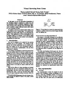
The simplest case of visual servoing combined with structured light consists of using a laser pointer attached to the camera. Let us consider the case of a planar object as shown in Figure 1.

where n = (A3 , B3 , C3 ) is the unitary normal vector to the plane. The expression of the depth Z corresponding to the intersection point between the object and the laser pointer can be obtained in a suitable form by solving the equations system built up with the planar object equation Π3 (6) and the normalised perspective projection equations x = X/Z, yielding D3 (7) Z=− A3 x + B3 y + C3 Applying the normalised perspective projection to the vectorial expression of the laser the following equations are obtained   xZ = Xr + λux yZ = Yr + λuy (8)  Z = Zr + λuz By summing the three equations we obtain Z(x + y + 1) = Xr + Yr + Zr + λ(ux + uy + uz ) (9) Then, by applying the depth Z in equation (7) and solving the equation for λ, its expression in function of the 3D parameters of the object and the origin of the ray is obtained as follows 1 λ = − (A3 Xr + B3 Yr + C3 Zr + D3 ) (10) µ with µ = nT u
= 0. Note that µ would be 0 when the laser pointer did not intersect with the planar object, i.e. when the angle between u and n is 90◦ . Thereafter, by taking into account that Xr and u do not vary in the camera frame, the time derivative of λ can be calculated yielding

Fig. 1. Case of a laser pointer linked to the camera and a planar object.

The interaction matrix Lx corresponding to the image point coordinates of the projected laser pointer was firstly formulated by Motyl et al. who modelled the laser pointer as the intersection of two planes [5]. However, the resulting matrix was in function of up to 12 3D parameters: 4 parameters for every one of the two planes defining the laser, and 4 additional parameters for the object plane. Even constraining the two planes modelling the laser to be orthogonal, the interpretation of the interaction matrix is not easy. A. Proposed modelling In order to reduce the number of 3D parameters involved in the interaction matrix, the laser pointer can be expressed in the following vectorial form (in the camera frame)

λ˙ = η1 A˙ 3 + η2 B˙ 3 + η3 C˙ 3 + η4 D˙ 3 with

 η1    η2 η  3   η4

= = = =

−(λux + Xr )/µ −(λuy + Yr )/µ −(λuz + Zr )/µ −1/µ

= −xZ/µ = −yZ/µ = −Z/µ

(11)

(12)

From the time derivatives of A3 , B3 , C3 and D3 involved in (11) given in [5], we have that (11) depends only on u, Xr , n, D3 and v. However, we can note that the unitary orientation vector u can be expressed in terms of the two points belonging to the line Xr and X as follows u = (X − Xr )/X − Xr 

(13)

where that u = (ux , uy , uz ) is an unitary vector defining the laser direction while Xr = (Xr , Yr , Zr ) is any reference point belonging to the line. The planar object is modelled according to the following equation

Applying this equation in (11), the resulting expression no longer depends on the explicit orientation of the light beam. The orientation is then implicit in the reference point Xr , the normalised point (x, y) and its corresponding depth Z. Afterwards, the computation of x˙ and y˙ is straightforward. First, deriving the vectorial equation of the light beam (5), the following equation is obtained

Π3 : A3 X + B3 Y + C3 Z + D3 = 0

˙ ˙ = λu X

X = Xr + λu

(5)

(6)

(14)

Then, if the normalised perspective equations are derived and the previous relationship is applied we find X˙ λ˙ X − 2 Z˙ ⇒ x˙ = (u − x · uz ) (15) Z Z Z After some developments, and choosing as reference point Xr = (X0 , Y0 , 0) we obtain the following interaction matrix x˙ =

 1 Lx = Π0

−A3 X0 Z

−B3 X0 Z

−C3 X0 Z

−A3 Y0 Z

−B3 Y0 Z

−C3 Y0 Z

 X0 ε1 X0 ε2 X0 ε3  Y0 ε1 Y0 ε2 Y0 ε1 (16)

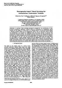
we propose a structured light sensor composed of four laser pointers. This choice has been taken because, as it will be demonstrated in the following section, a decoupled control scheme can be achieved by a suitable spatial configuration of the four lasers. Concretely, we propose to position the lasers forming a symmetric cross centred in the focal point of the camera, so that the axis of the cross are aligned with the X and Y axis of the camera, as shown in Figure 2. Furthermore, we propose to set the direction of the lasers coinciding with the optical axis Z of the camera. The distance of every laser origin to the camera focus is called L. Such lasers

where

inria-00352034, version 1 - 12 Jan 2009

Π0 ε1 ε2 ε1

= = = =

A3 (X0 − xZ) + B3 (Y0 − yZ) − C3 Z B3 − yC3 C3 x − A3 A3 y − B3 x

Note that with respect to the interaction matrix proposed by Motyl et al. in [5], the number of 3D parameters concerning the laser beam has been reduced from 8 to 3, i.e. X0 , Y0 and Z. The orientation of the beam remains implicit in our equations. Concerning the planar object, the number of parameters has been reduced from 4 to 3 since D3 has been expressed in function of the image coordinates (x, y), the corresponding depth Z of the point and the normal vector to the planar object. From (16) we directly obtain that the rank of the interaction matrix Lx is always equal to 1, which means that the time variation of the x and y coordinates of the observed point are linked. Thus, the image point moves along a line as pointed out by Andreff et al. [1].

1 4

Yc

Zc

Xc

Fig. 2.

Laser pointers configuration.

configuration produces a symmetric image like shown in Figure 3 when the image plane is parallel to the planar object, i.e. for the desired position. Given this lasers conxp

3

yp

III. T HE PROPOSED STRUCTURED LIGHT SENSOR In this section we deal with the problem of positioning a camera parallel to a planar object by using only visual data based on some projected structured light. A plane has only 3 degrees of freedom, which means that only three axes of the camera will be controlled (or three combinations of the 6 axis). In this section we propose a structured light sensor based on laser pointers which intends to achieve three main objectives: decoupling of the controlled degrees of freedom (at least near the desired position), robustness against image noise and control stability, and improving the camera trajectory by removing non-linearities in the interaction matrix. The choice of a structured light sensor based on laser pointers implies the choice of the number of lasers and how they are positioned and oriented with respect to the camera. In theory, three laser pointers are enough in order to control 3 degrees of freedom. The positioning of such lasers must be chosen in order to avoid three collinear image points, which would lead to a singularity in the interaction matrix. A simple way to avoid such situation is to position the lasers forming an equilateral triangle so that all the lasers point towards the same direction. However,

2

3

Xc

2 Yc

Fig. 3.

4

1

Example of image when the camera and the object are parallel.

figuration, the coordinates of the reference points (origin) of every laser, and the normalised image coordinates of the projected points are shown in table I. TABLE I L ASER REFERENCE POINT COORDINATES AND NORMALISED IMAGE POINT COORDINATES ( CAMERA FRAME ) Laser 1 2 3 4

X0 0 -L 0 L

Y0 L 0 -L 0

Z0 0 0 0 0

x∗ 0 -L/Z 0 L/Z

y∗ L/Z 0 -L/Z 0

IV. O PTIMISING THE INTERACTION MATRIX Finding a set of visual features which produces a decoupled interaction matrix for any camera pose seems an

unreachable issue. However, we can find visual features which show a decoupled behaviour near the desired position. In this section we propose a set of 3 visual features which produce a decoupled interaction matrix with low condition number and which removes the non-linearities for all the positions where the image plane is parallel to the object. The first visual feature of the proposed set is the area enclosed in the region defined by the four image points. The area has been largely used to control the depth as in [2], [7], [10]. In our case, the area formed by the 4 image points can be calculated by summing the area of the triangle defined by the points 1, 2 and 3, and the area of the triangle defined by 3, 4, and 1. After some developments we obtain the following formula

inria-00352034, version 1 - 12 Jan 2009

a=

1 ((x3 − x1 )(y4 − y2 ) + (x2 − x4 )(y3 − y1 )) (17) 2

that only depends on the point coordinates, whose interaction matrices are known. After some developments, the interaction matrix of the area when the camera is parallel to the object can be obtained as follows La

= (

0

4L2 /Z 3

0

0 0 0 )

(18)

We can note that when the camera is parallel to the object, the 3D area enclosed by the 4 projected points is equal to A = 2L2 , independently of the depth Z. This is true because the laser pointers have the same direction than the optical axis. Then, knowing that the image area is a = A/Z 2 the interaction matrix La can be rewritten as La

=

(

0

0

2a/Z

0 0 0 )

(19)

The 2 visual features controlling the remaining degrees of freedom are selected from the 4 virtual segments defined according to the Figure 4. xp yp

l32 2

α2 l12

α1 1

l34 α4 l14

i

K Y

4 j

αj

K X

k

Fig. 4. At left side, virtual segments defined by the image points. At right side, definition of the angle αj .

An interesting feature is the angle between each pair of intersecting virtual segments. The angle αj corresponding to the angle between the segment ljk and the segment lji (see Figure 4) is defined as → − → u ×− v sin αj = → − → v  u −

→ − → u ·− v , cos αj = → → u − v −

(xk − xj )(yi − yj ) − (xi − xj )(yk − yj ) (xk − xj )(xi − xj ) + (yk − yj )(yi − yj ) (21) Knowing that the derivative of f (x) = arctan(x) is f˙(x) = x/(1 ˙ + x2 ), the interaction matrix of αj can easily be calculated. Then, by choosing the visual features α13 = α1 − α3 and α24 = α2 −α4 , the following interaction matrices are obtained when the camera is parallel to the object. αj = arctan

Lα13 Lα24

= ( 0 0 0 2L/Z = ( 0 0 0 0

0 2L/Z

0 ) 0 )

(22)

Note that by using the visual feature set s = ( a, α13 , α24 ) the interaction matrix is diagonal (for the desired position) so that a decoupled control scheme is obtained with no singularities. However, it can be also noted that the non-null terms of the interaction matrix are inversely proportional to the depth Z. This will indeed cause the camera trajectory not to be completely satisfactory. As pointed out by Mahony et al. [7], a good visual feature controlling one degree of freedom (dof) is that one whose error function should vary proportionally to the variation of the dof. Let’s start by searching a feature an whose time derivative only depends on constant values. Since the time derivative of a depends on the inverse of the depth, we can search a feature of the form an = aγ so that the depth is cancelled in its time derivative. Then, taking into account all this, the required power γ can be deduced as follows 2γAγ (23) an = aγ ⇒ a˙ n = γaγ−1 a˙ = 2γ+1 · Vz Z In order to cancel the depth it is necessary that 2γ + 1 = 0 ⇒ γ = −1/2

(24) √ Therefore, the interaction matrix of an = 1/ a is √ Lan = ( 0 0 −1/( 2L) 0 0 0 ) (25) Following the same methodology, it can√be found that by choosing as visual features αn13 = α13 / a and αn24 = √ α24 / a the following constant matrices are obtained √ 2 0 0 ) Lα13n = ( 0 0 0 √ (26) Lα24n = ( 0 0 0 0 2 0 )

3 α3

Then, developing the inner and outer product, the angle is obtained from the point coordinates as follows

(20)

V. C OMPARISON WITH THE IMAGE POINTS APPROACH In this section the performance of the proposed set of visual features is compared with the set composed of the normalised image point coordinates. The comparison is made from an analytical point of view by calculating the local stability conditions around the desired position. The conditions of stability are expressed in function of the parameters describing the misalignment between the laserscross frame and the camera frame. This misalignment is modelled according to the following transformation matrix 

c Rl c Tl c (27) Ml = 03 1

inria-00352034, version 1 - 12 Jan 2009

The local stability analysis takes the closed-loop equation of the system in the desired state [8]

domain when using the proposed visual features is larger than when using simple image points coordinates.


∗ )−1 e e˙ = −λCL∗s (CL s

VI. E XPERIMENTAL RESULTS

(28)


∗ is the model of the interaction matrix in the where L s desired position where the laser-cross is supposed to be perfectly aligned with the camera frame. On the other hand, L∗s is the real interaction matrix in the desired position taking into account the misalignment of the laser-cross described by the frame transformation in equation (27). Then, the local stability is ensured when the product of matrices in the closed-loop equation is definite positive. We remember that a matrix is definite positive if the eigenvalues of its symmetric part have all positive real part. In practice, if a whole model of misalignment is considered, the analytical computation of the eigenvalues becomes too complex, so we face the stability analysis by considering a simplified model where the laser-cross frame is only displaced with respect to the camera frame. Then, the transformation matrix between both frames in equation (27) is such that c Rl = 03 and c Tl = (x , y , z ). Applying this simplified misalignment model to the laser-cross frame, the reference points and normalised image coordinates shown in table II are obtained when the camera is parallel to the object. These parameters are used to calculate L∗s , while the ideal parameters (assuming perfect alignment of both frames) in table I are used to
∗ . Since both interaction matrices have null calculate L s values for Vx , Vy and Ωz , they can be reduced to 3 × 3 matrices, so that C can be chosen as the identity matrix. TABLE II L ASER ORIGINS AND POINT COORDINATES Laser 1 2 3 4

X0 x -L+x x L+x

Y0 L+y y -L+y y

Z0 z z z z

x∗ x /Z (x − L)/Z x /Z (L + x )/Z

y∗ (L + y )/Z y /Z (y − L)/Z y /Z

First of all we test the local stability conditions for the set of visual features composed of the normalised image point coordinates s = (x1 , y1 , x2 , y2 , x3 , y3 , x4 , y4 ). Calculating the eigenvalues of the symmetric part of the
∗ )−1 and imposing their positivity, the folproduct L∗s (L s lowing condition arises 2x + 2y < 2L2

(29)

which √ is nothing else that the equation of a circle with radius 2L. Note that z does not affect the local stability, while a displacement of the laser-cross centre in the plane XY is tolerated if it is included in this circle. If the local stability analysis is made for the proposed set of visual features s = (an , α13n , α24n ) all the eigenvalues are equal to 1. This means that the local stability when using this set of visual features is always ensured when the laser-cross is only displaced with respect to the focal point. Such analytical results demonstrate that the stability

In this section the performance of the proposed set of visual features is compared with the case when image points are directly used. The experimental setup consists of a six-degrees-of-freedom robot with a camera coupled to its end-effector. The laser-cross structure has been built so that each laser pointer is placed at L = 15 cm from the cross intersection. The goal of the task consisted of positioning the camera parallel to a plane placed in front of the robotic cell at a distance of 95 cm. The desired image was acquired by positioning the robot in such a desired position. The first experiment consisted of moving the camera far away from the desired position about 20 cm and rotations of −40 and 20 degrees were applied with respect to the X and the Y axis, respectively. The results of the servoing by using the normalised image coordinates of the four laser points are shown in Figure 5a while the results when using the proposed visual features are presented in Figure 5b. As can be seen in the final images, the lasers are not perfectly aligned with the camera frame producing a non-symmetric image. However, the misalignment of the laser-cross is small enough to allow the convergence of the system even when using image point coordinates. As expected, the trajectories of the lasers points in the image are straight lines. The approach based on image points presents an almost exponential decrease of the error. However, the camera kinematics show a non-pure exponential behaviour. This fact is due to the non-linearities in the interaction matrix based on image points. On the other hand, as expected, a pure exponential decrease of the error in the visual features, as well as in the camera velocities, is observed in the case of the proposed set of visual features. In terms of numeric conditioning, the interaction matrix based on image point has a condition number equal to 11.17, while for our set of visual features the condition number is 3.3. A second experiment was carried out in order to test the sensitivity of the system to the alignment between the camera and the lasers-cross. Concretely, the laserscross was displaced about 6 cm along the X axis of the camera frame. Then, the camera was moved backwards from the desired position about 40 cm and rotated −20 and 20 degrees around the X and Y axis respectively. With such a large misalignment of the lasers-cross, the approach based on image point coordinates rapidly failed. Meanwhile, the approach based on our set of visual features still converged as shown in Figure 5c. The image trajectories of points 1 and 3 are no longer parallel to the Y axis due to the misalignment. The control on depth and on Ωx are almost unaffected by the cross misalignment. However, the feature α24n controlling Ωy presents a nonpure exponential decrease because it is certainly affected by the large misalignment. The robustness of the proposed visual features against large misalignment errors of the lasers-cross was already

a) 0.06

0.06

*

x1-x1* y1-y1 * x2-x2* y2-y2* x3-x3* y3-y3 x4-x4* y4-y4*

0.04 0.02 0

Vz Ωx Ωy

0.04 0.02 0

-0.02

-0.02

-0.04 -0.04 -0.06

0

5

10

15

20

25

0

5

10

15

20

25

b) 3

0.15

*

Vz Ωx Ωy

an-an

2.5

* 13n * α24n-α 24n

α13n-α

2 1.5

0.1

0.05

1 0.5

0

0 -0.5

-0.05

-1 -1.5 0

5

10

15

20

0

25

5

10

15

20

25

c) 2

an-an*

1.5

Vz Ωx Ωy

0.15

* 13n α24n-α*24n

α13n-α

1

0.1

0.5 0.05

inria-00352034, version 1 - 12 Jan 2009

0 -0.5

0

-1 -1.5

0

5

10

15

20

25

-0.05

0

5

10

15

20

25

Fig. 5. a) 1st experiment using image point coordinates, b) 1st experiment using the proposed visual features, c) 2nd experiment. Each column shows (from left to right): initial image; final image (with the trajectories of the laser points); visual features s − s∗ versus time (in s); camera velocities (m/s and rad/s) versus time (in s)

expected from the local stability analysis. Furthermore, we can intuitively understand this robustness because the area and relative angles defined upon the 4 image points are invariant to 2D rotations, translations and scaling (when the image plane is parallel to the target and all the lasers have the same orientation). VII. C ONCLUSIONS In this paper the task of positioning a camera parallel to a planar object has been faced. An approach based on visual servoing combined with structured light has been presented. Thanks to the flexibility of using structured light, the system behaviour has been optimised in three main aspects: control stability and decoupling, well-conditioning and better controlled camera velocities. The structured light sensor proposed is composed of four lasers pointers which are placed symmetrically with respect to the camera and pointing towards the same direction than the optical axis. Such configuration is suitable for defining a set of 3 decoupled visual features (near the desired position) which guarantees a higher degree of robustness against the lasers calibration than when using image point coordinates. Furthermore, non-linearities in the interaction matrix are removed producing a better mapping from the feature space to the camera velocities. The better performance of our approach in front of image point coordinates has been demonstrated through a local stability analysis and experimental results.

VIII. ACKNOWLEDGMENTS Work partially funded by the Cemagref Rennes of France and the Ministry of Universities, Research and Information Society of the Catalan Government. R EFERENCES [1] N. Andreff, B. Espiau, and R. Horaud. Visual servoing from lines. Int. Journal of Robotics Research, 21(8):679–700, August 2002. [2] P. I. Corke and S. A. Hutchinson. A new partitioned approach to image-based visual servo control. IEEE Trans. on Robotics and Automation, 17(4):507–515, August 2001. [3] J. T. Feddema, C. S. G. Lee, and O. R. Mitchell. Weighted selection of image features for resolved rate visual feedback control. IEEE Trans. on Robotics and Automation, 7(1):31–47, February 1991. [4] S. Hutchinson, G. Hager, and P. Corke. A tutorial on visual servo control. IEEE Trans. on Robotics and Automation, 12(5):651–670, 1996. [5] D. Khadraoui, G. Motyl, P. Martinet, J. Gallice, and F. Chaumette. Visual servoing in robotics scheme using a camera/laser-stripe sensor. IEEE Trans. on Robotics and Automation, 12(5):743–750, 1996. [6] A. Krupa, J. Gangloff, C. Doignon, M. Mathelin, G. Morel, J. Leroy, L. Soler, and J. Marescaux. Autonomous 3d positionning of surgical instruments in rototized laparoscopic surgery using visual servoing. IEEE Trans. on Robotics and Automation, 19(5):842–853, 2003. [7] R. Mahony, P. Corke, and F. Chaumette. Choice of image features for depth-axis control in image-based visual servo control. In IEEE/RSJ Int. Conf. on Intellingent Robots and Systems, Lausanne, Switzerland, September 2002. [8] E. Malis, F. Chaumette, and S. Boudet. 2 1/2 d visual servoing. IEEE Trans. on Robotics and Automation, 15(2):238–250, April 1999. [9] J. Salvi, J. Pag`es, and J. Batlle. Pattern codification strategies in structured light systems. Pattern Recognition, 37(4):827–849, 2004. [10] O. Tahri and F. Chaumette. Image moments: Generic descriptors for decoupled image-based visual servo. In IEEE Int. Conf. on Robotics and Automation, volume 2, pages 1185–1190, New Orleans, LA, April 2004.