Image Based Visual Servoing from Groups of 3D points

ISR 2004 Paris France March 26-April 1

Image Based Visual Servoing from Groups of 3D points ∗

Florian Schramm∗,† , Guillaume Morel∗ , Anne Lottin† Laboratoire de Robotique de Paris, Fontenay-aux-Roses, France † CEA - LIST, Fontenay-aux-Roses, France

Abstract— This paper presents a new approach for eye-in-hand visual servoing. The error to be controlled represents 3D feature points for a system with unknown, but constant camera calibration. It does not require more information than the original image based scheme, but exploits it more exhaustive: Depth information is incorporated into the error vector. This allows for the main contribution: a formal demonstration of globally asymptotical stability for the proposed image based control law. The paper details how for a vector of non-metric 3D point coordinates and a standard controller based on the transposed of the Image Jacobian all possible undesired equilibria, namely three, can be determined analytically and shown to be unstable.

I. I NTRODUCTION Within the framework of monocular hand-in-eye visual servoing, originally image based and pose based approaches are distinguished. In the original pose based approaches ([1], [2]), a reconstruction algorithm is present in the control loop in order to provide a camera pose as error vector to be controlled and prevents from robustness analysis w.r.t. to camera intrinsic parameters. Only recently, due to the projective reconstruction algorithm [3], robust controllers have been proposed ([4], [5], [6]). However, the assumptions for the involved partial reconstruction algorithm are not always satisfied in practice, namely to dispose of a plane at infinity. As for those pose based approaches not requiring a target model, image based approaches rely on an a priori learnt image, taken in the desired configuration. Then the control error vector measures image feature distance from the current to the desired view. Originally image based approaches, using 2D image point features, are experimentally known to be locally robust – controlled error is naturally independent of the constant intrinsic camera parameters – but to suffer from singularities and undesired equilibria (even attractive ones!) [7]. To alleviate these drawbacks, controller based on other image features are proposed [8], [9], [10]. Again, none of them provides a formal stability analysis. For image based approaches, extracted and matched features from two views are sufficient to state the error vector – however, for the corresponding Image Jacobian, relating variations of image features and control, usually a kinematic screw for camera motion, much more information is required, namely some metric information of the image feature including depth [11] and hence calibration. Then, it comes at no cost to use depth information in the error vector ([1], [12], [9]), extending two 2D image points to non-metric 3D image points. Such

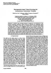
coordinates have most recently [12] formally shown to allow for an image based controller which does not suffer from singularities nor undesired equilibria, at least locally, i.e. for a limited orientation error. We pursue a similar approach, since our control design is based on the same non-metric 3D point coordinates. For unknown intrinsic camera parameters, we determine all three undesired equilibria, i.e. configurations, where the error vector lies in the null space of the transpose image Jacobian. Then we show formally them to be locally unstable. We assume depth of all points to be available up to a scalar factor. Under a weak visibility assumption, a pseudo linearizing controller can be shown in practice to globally asymptotically stabilize any desired final configuration, whatever the actual values for the intrinsic camera parameters may be. three undesired equilibria are excluded as starting point; two of them are however not reachable from the current visibility half sphere. To our knowledge, this is the first image based visual servoing control to be globally asymptotically stable wrt. calibration errors and relative depth errors. II. M ODELLING AND C ONTROL D ESIGN The well known problem of eye-in-hand visual servoing is depicted in Fig. II. Target object with arbitrary points

Image plane si

sdes,i

pi ez

F

Optical camera center R, t

pdes,i ez

Fdes Fig. 1.

Problem statement

A. Camera A camera, rigidly mounted on the tip of a manipulator, is to moved such that the attached frame F (also called the current

ISR 2004 Paris France March 26-April 1 frame), coincides with a desired camera frame Fdes . It is assumed that an image of the tracked target in the desired pose has been learnt prior to the visual servoing task, and that a vision algorithm allows to extract, in real time, image coordinates for a set of m matched points between the current and the desired image. No object model is required. A pinhole model of the camera is used. Given a target point Pi , we have: 1 (1) pi = Axi zi where pTi = [ui vi 1] groups the pixel image coordinates ui , vi of Pi , xTi = [xi yi zi ] groups the coordinates of Pi in F and A groups the intrinsic camera parameters:   αu αuv u0 αv v0  A=0 (2) 0 0 1 B. State vector In order to build our state vector, we have to assume that enough information is available in the image. As we will see later on, our control approach requires at least three non aligned points of the tracked target to be visible at any time of the task. Assumption 1: The tracked target consists of m ≥ 3 physical points, that can be localized by the vision system. They are (at any time) visible in both the desired and the current image. They are correctly matched, and at least three of them are not aligned in the image. ¤ The assumption that at least three of the points in the image plane are not aligned is weak. Indeed, the only solution for the (non physically aligned) target points to project into a straight line is that the target is planar, and the camera frame belongs to the target plane. However, this configuration is clearly at the limit of the visible workspace. Finally, note that the occlusion problem is not addressed in this work. For a given point Pi , we introduce non-metric 3D coordinates si , based on an estimate zˆi of its depth and an estimate ˆ of the camera calibration matrix A: A ˆ −1 pi si := zˆi A

(3)

Clearly, si can be seen as an estimate of xi , since si ≡ xi ˆ ≡ A and perfect depth in the case of perfect calibration A estimation zˆi ≡ zi . Grouping the coordinates (3) of the m target points into a single vector yields the state vector: sT = [sT1 sT2 . . . sTm ]

(4)

It shall be emphasized that the requirement for an estimate of the discrete depth field Z = [z1 z2 . . . zm ] does not imply the need for a pose reconstruction algorithm. Rather, several algorithms [3] can estimate Z from two views on the point set P1 , . . . Pm , corresponding to a rigid target. As we suppose to ignore the exact intrinsic camera parameters, algorithms are based on exploiting additional information, either of the scene (points at infinity, physically parallel lines, planar target), either of a particular motion between the two views (pure

translation, pure rotation). In any case, the elements of the discrete depth field Z can be estimated up to a common constant scalar factor ζ, zˆi = ζzi

(5)

Then, the new coordinates (3) for any Pi are: ˆ −1 pi = ζ zˆiδAA−1 pi si = zˆi A

(6)

ˆ represents the calibration error matrix. The where δA := AA ˆ δA are all upper triangular with strictly posmatrices A, A, itive diagonal entries. One can see that there exists a constant linear relationship between si and metric 3D coordinates xi : si = ∆xi ,

with ∆ := ζδδA

(7)

Again, ∆ and its inverse are both upper triangular constant matrices, with positive diagonal entries. We finally get:     x1 ∆ 03     .. s = D  ...  with D =  (8)  . xm

03

∆

C. Image Jacobian and its estimate Control action is assumed to be the usual absolute kinematic screw of the camera, expressed in camera coordinates: · ¸ · ¸ v v(Oc ∈ F/Fo ) u= = (9) ω ω (F/Fo ) where v(Pi , Fk /Fj ) denotes the translational velocity of point Pi in the motion of Fk relatively to Fj and ω (Fk /Fj ) denotes the angular velocity of Fk relatively to Fj . Frame Fo is attached to the tracked target, which is always at rest. The Image Jacobian J is defined as: x˙ = J(x)u

(10)

where xT = [xT1 xT2 . . . xTm ]. Since xi represents the target point Pi in camera frame F, we have: x˙ i = v(Pi , F/Fo ) = −v(Pi , Fo /F) = −v − ω × xi Or, in matrix form, £ x˙ i = −I3

[xi ]×

¤

(11)

where [a]× b ≡ a × b. For all points Pi together, we obtain:   −I3 [x1 ]× −I3 [x2 ]×    J(x) =  . (12) ..   .. .  −I3

[xm ]×

ˆ that will be used in the control Naturally, the estimate J, ˆ are law, is built up under the tacite assumption that zˆi and A ˆ known without errors. Thus we use an estimate J based on the new coordinates si (3) for the image jacobian: ˆ := J(s) J

(13)

ISR 2004 Paris France March 26-April 1 By [si ]× = [∆xi ]× = det(∆)∆−T [xi ]× ∆−1 , we get: ˆ = J(s) = D−T J(x)F J where F is regular as long as ∆: · T ¸ ∆ I3 F= I3 det(∆)∆−1

(14)

(15)

D. Proposed controller The goal of the visual servoing task is to bring the current configuration s to a previously captured configuration sdes . Therefore, the control error is defined as: e := s − sdes

(16)

Since matrix D is regular, we have from (8): e=0

⇔

xi = xdes,i for i = 1, 2, . . . , m

(17)

where xdes,i = ∆−1 sdes,i is the position of point Pi in the camera frame of the desired configuration. Furtermore, it is well known that if three nonaligned points of a rigid body coincide in two different frames, then the two frames coincide. The reciprocal is trivial. Thus, from assumption 1, the following property holds: Property 1: The error e = s − sdes is zero iff F ≡ Fdes . ¤ Note that the ambiguity usually encountered in conventional image based control using three image points does not hold any more when using the new coordinates si for the error vector, incorporating depth information. Two critical issues of conventional image based approaches, namely local minima and global stability, will be remedied by the use of the coordinates si . To this end, we use the controller: ˆT

u = λJ e

(18)

where λ is a constant diagonal gain matrix. III. P ROPERTIES OF THE CONTROL LAW In order to provide a stability analysis of the control law, we first derive two properties, related to the rank and the Null ˆ space of the estimated image jacobian J. ˆ A. Rank of the Image Jacobian J £ T T ¤T ˆ ∈ R6 be a vector verifying J(s)a = 0, Let a = a1 a2 and let Pα , Pβ and Pγ be three non aligned points of the target. Thanks to assumption 1, these points exist and their 3D coordinates xα , xβ and xγ necessarily span R3 . Indeed, the vectors xα , xβ and xγ can neither be colinear (points not aligned) nor be coplanar (which would imply that Oc , Pα , Pβ and Pγ lie in the same plan). Thus, thanks to the regularity of ∆, the vectors sα , sβ and sγ also span R3 . Furthermore, ˆ since we assumed J(s)a = 0, we have:  ½  −a1 + [sα ]× a2 = 0 [sα − sβ ]× a2 = 0 −a1 + [sβ ]× a2 = 0 ⇒ (19) [sβ − sγ ]× a2 = 0  −a1 + [sγ ]× a2 = 0 Then, necessarily, a2 = 0, which in turn implies that a1 = 0. ˆ To summarize, if J(s)a = 0, then necessarily a = 0, ˆ which proves J(s) to be of full column rank 6. Consequently,

ˆ T J(s) ˆ is of rank 6 and, given the regularity of D, DJ(x)T J(s) is of rank 6 as well. ˆ ˆ T J(s) ˆ J(s) Property 2: If Assumption 1 is verified, J(s), and J(x) are all of rank 6. ¤ ˆT B. Null space of image Jacobian J Within visual servoing applications, any 2D image based controller exhibits undesired equilibrium configurations. In such a configuration, the error vector is not zero, but the controller output u is zero – hence the system does not move. Moreover, in 2D image based control, some configurations characterizing undesired equilibria haven been experimentally found to be attractive (i.e. locally stable), providing a local minimum from which the controller cannot move. More precisely, an undesired equilibrium occurs when e lies in ˆT . In our case, J ˆT is a 6 × 3m matrix the null space of J T ˆ = 6, hence the dimension of the null space with rank J is 3m − 6 ≥ 3. Mathematically, undesired equilibria ˜ s are solutions s = ˜ s of ˆ T e = J(s) ˆ T (s − sdes ) = 06×1 J(s)

(20)

ˆT lacks However, whether e can lie or not int null space of J of a trivial answer, because e = s − sdes is not an arbitrary vectors of R3 . Rather, they are subject to a rigid body motion constraint. First, let us notice from (14) that: ˆ s)T e = FT J(˜ J(˜ x)T D−1 e = FT J(˜ x)T (˜ x − xdes )

(21)

−1

where x ˜ = D ˜ s. Thus, F being non singular, undesired equilibria are solutions of J(˜ x)T (˜ x − xdes ) = 06×1

(22)

under the constraint ∃ R, t s.t. x ˜i = Rxdes,i + t for i = 1, 2, . . . , m

(23)

where the rotation matrix R and the translation vector t describe, in the camera frame, the displacement of the target from the desired configuration to an (yet unknown) undesired equilibrium configuration. Interestingly, the undesired equilibria are not affected by the calibration uncertainties. Recalling Rodriguez formula R = I3 + sin θ[νν ]× + (1 − cos θ)[νν ]×2

(24)

T

and therefrom R − R = 2 sin θ[νν ]× , the rigid displacement constraint yields: x ˜i − xdes,i = (I3 − RT )˜ xi + RT t T

1

xi ]× R 2 ν sin θ + RT t = −R 2 [˜ where ν and θ are the unitary axis and the angle of rotation of R = exp(θνν ). Thus:   T 03 −R 2 ¸ · T R2t   .. (25) J(˜ x ) x ˜ − xdes =  1  . R 2 ν sin θ T } {z | 03 −R 2 w } {z | Q

ISR 2004 Paris France March 26-April 1 with:

Eq. (22) can now be rewritten as: J(˜ x)T QJ(˜ x)w = 0

(26)

Clearly, a solution is given by the desired final configuration θ = 0, t = 0, which represents an equilibrium. Further, undesired, equilibria (θ 6= 0, t 6= 0) cannot arise from considering only J(˜ x)w = 0, since J(˜ x) is of full rank 6 as shown in section III-A. Rather, undesired equilibria are characterized by J(˜ x)T QJ(˜ x) being singular, wT J(˜ x)T QJ(˜ x)w =

m X

T

zTi R 2 zi = 0

[zT1

zT2

zTm ]

T

T

∀i = 1, 2, . . . , m T 2

(28) π 2.

hence the only solution is R to be a rotation of In the rest of this section we will compute rotation axis ν characterizing jointly with θ = π undesired equilibria configuration. With θ = π, (24) simplifies to R = I3 + 2[νν ]×2 = 2νν ν T − I3

(29)

Combining with (23), the first block line of (22) becomes: m ¢X ¡ ¢ 1¡ I3 − R xdes,i = 2 I3 − ν ν T x ¯des (30) t= m i=1 Pm 1 where we have set x ¯des = m i=1 xdes,i . Furthermore, the second block line of (22) yields:

0=

m X

[Rxdes,i + t]× xdes,i

i=1

=

m X

[Rxdes,i ]× xdes,i − m[R¯ xdes ]× x ¯des

(31)

i=1

Due to the particular structure of R (cf. 29), we have for any vector a ∈ R3 : ¡ ¢ −[Ra]× a = [a]× 2νν ν T − I3 a = 2[(aaT )νν ]×ν Therefore, eq. (31) gives: · ³X ¸ m ¡ ¢ ¡ ¢´ xdes,i xTdes,i − m x ¯des x ¯Tdes ν ν = 0

(32)

×

i=1

Then, ν is sufficiently and necessarily an eigenvector of the matrix C given by: C=

m X ¡

xdes,i xTdes,i

¢

¡ ¢ −m x ¯des x ¯Tdes

(33)

i=1

To summarize this section: Property 3: For a given desired configuration sdes satisfying assumption 1, there are only four solutions ˜ s for J(˜ s)T (˜ s− sdes ) ≡ 0 corresponding to a feasible rigid motion. One solution is the desired equilibrium ˜ s = sdes . The three other solutions k = 1, 2, 3 are given by ˜ s = D˜ x, where x ˜i = Rk xdes,i + ti

ν k = eigvect

m X 1 (I3 − Rk ) xdes,i m i=1

m X ¡ ¢ ¡ ¢ xdes,i xTdes,i − m x ¯des x ¯Tdes i=1

¤ IV. S TABILITY ANALYSIS

T

= w J(˜ x) . Since all where z = ... summands have the same sign it follows zTi R 2 zi = 0

tk = (I3 − Rk )¯ xdes =

(27)

i+1 T

xdes,i = D−1 sdes,i Rk = exp(πνν k ) = I3 + 2[νν k ]×2

for i ∈ {1, 2, . . . , m}

(34)

In order to provide a stability analysis, we first derive the closed loop behaviour of x, which groups the 3D metric point coordinates. From (12,18), we obtain: x˙ = J(x)u = −λJ(x)FJ(x)T (x − xdes ) =: f (x)

(35)

Next, the undesired equilibrium x = x ˜ is studied, and afterwards the stability of the desired minimum x = xdes . A. Stability of undesired equilibria We can develop f (x) in (35) around x = x ˜ by : · ¸ ∂f (x − x ˜) + O(x2 ) x˙ = f (x) = x(˜ x) + ∂x x˜ | {z }

(36)

=:U

The linearized system is thus x˙ = U(x − x ˜)

(37)

where xi,j is the j th component of xi . We have: ¯ ¯ ∂(J(x)FT ) ¯¯ ∂f ¯¯ ˜x J(˜ x)T e = −λ ∂xi,j ¯x˜ | {z } ∂xi,j ¯x˜ =0 ¯ ¾ ¯ ½ T¯ ¯ ∂J(x) ¯ T ∂x ¯ ˜ (38) e + J(˜ x ) − λJ(˜ x)FT x ¯ ∂xi,j ¯x˜ ∂xi,j x˜ ˜x = (˜ where we have set e x − xdes). We have: £ ¤T ∂x = · · · 0T3×1 kTj 0T3×1 · · · ∂xi,j

(39)

on the ith position kTj the canonical basis (k1 , k2 , k3 ). Then: · ¸ ∂x −I3 = k JT (˜ x) −[˜ x]× j ∂xi,j Moreover, from (12), we have: ¯ · ¸ · ¸ ∂J(x)T ¯¯ 03×1 03 ˜ ex = = k ˜ xi − [kj ]× e [˜ exi ]× j ∂xi,j ¯x˜ Summing the preceding two eqns., we get: ¯ ¯ · ¸ ∂x ¯¯ ∂J(x)T ¯¯ −I3 T ˜ = k e + J (˜ x ) x −[xdes,i ]× j ∂xi,j ¯x˜ ∂xi,j ¯x˜ Inserting the last eqn. in (38), and grouping into a matrix form, we finally get: U = −λJ(˜ x)FT J(xdes )T

(40)

ISR 2004 Paris France March 26-April 1 We shall now prove, that the matrix U has at least one strictly positive eigenvalue. Let Pk , Pj be two target points ¡ ¢T ¡ ¢ verifying xdes,k 6= xdes,j and xdes,k − xdes,j x ˜k − x ˜j 6= 0. They necessarily exist since, by assumption 1, the tuple {x1 , x1 , . . . , xm } spans R3 . Now consider the vector: # " µT0 0 . . . 0 µT0 0 . . . 0 −µ 0 . . . 0 −µ T | {z } | {z } (41) c0 =

[11], deterioring calibration – required for the metric information for the Image Jacobian – may cause the control to fail. to our knowledge, the global asymptotic stability of a non pose based visual servoing approach to a 6 dof positioning problem is unique in the literature, even in a perfect calibration case.

•

V. S IMULATION RESULTS

j th vect.

kth vect.

where µ 0 = xdes,i − xdes,j + x ˜i − x ˜j . One can show that: · ¸ 03×1 T J(xdes) c0 = =: c1 (42) [˜ xk − x ˜j ]× (xdes,i − xdes,j )

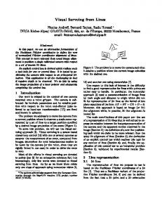
The following simulation results illustrate the above shown properties of the visual servoing law, namely the lack of local minima and the global asymptotical stability. a:Camera traj. in the target frame (m)

Therefore:

b: Traj. of the target in the camera frame (m)

0.5

cT0 Uc0 = λcT1 FT c1

(43)

Clearly, since F is positive definite, we have: cT0 Uc0

>0

1 0.8

0

0.6 0.4

−0.5

(44)

0.2 −1 0.2

0

which shows that at least one of the eigenvalues of U is strictly positive, i.e. the linearized system (37) being unstable.

−0.2

0.5

0

−0.5

0

c: Image trajectory (pixels) vs time (s)

−0.2

0.2

0

−0.2

d: Estimated error (m) vs t (s)

400

B. Stability of the desired minimum

0 0.2

0.05

300

Consider now the following Lyapunov candidate: 1 (45) V = (x − xdes)T (x − xdes), 2 which is null only at the desired configuration thanks to Property 1. Its time derivative is given by: V˙ = (x − xdes)T x˙ = zT FT z

(46)

200

0

100

0

0

200

400

600

0

10

Trans. velocity (m/s) vs t (s)

20

30

40

50

Rot. velocity (deg/s) vs t (s)

1 150

0.5

100

0

where we have set z = J(x)T (x − xdes). Now, invoking Property 3, the vector z is null for only four configurations, the three undesired configurations of equilibrium and the desired equilibrium x = xdes. As shown above, the three undesired equilibria are unstable providing that F is positive definite. Finally, beside these four configurations, a sufficient condition for V˙ to be negative is that F remains positive in all the visible trajectories. Then, V is a Lyapunov function. We summarize the results of section IV: Property 4: Under assumption 1, for the closed loop system (35) to be globally asymptotically stable, it is sufficient not to start in an undesired equilibrium (cf. Property 3) and to ensure F to be positive definitive, which means the focal distance is assumed to be positive, hence including the perfect calibration case. ¤ Finally, let’s emphasize that: • the positive definitiveness of F, which is sufficient for the controller to yield global asymptotic stability, is equivalent to the positive definitiveness of δA (cf. 8). One then find the same conditions as [4]. • Precisely speaking, we even need lees information than the original 2D image based approach, since the proposed control works fine even if the depth distribution is known up to a scale factor and the calibration totally ignored. Contrarily for the original 2D imaged based scheme

−0.05

50

−0.5 −1

0

−1.5

−50

−2

−100

−2.5 −3

−150 0

10

Fig. 2.

20

30

40

50

0

10

20

30

40

50

Perfect calibration: Task with small displacement

A general, non flat target constituted by 6 points has been used, with 2D point coordinates [−a − a 0], [a − a 0], [a a 0], [0 2a 0], [−a a 0], [0 0 − a] where a = 5cm. For a first¤ task, perfect calibration has been assumed, A = £ 2000 0 0 0 2000 0 . Fig. (2) shows the system behavior: The feature 0 0 1 points Pi are tracked by blue thick lines in camera space (b) and on the image plane (c). With in the target frame, characterized by the upper trihedron in (a), initial and final camera configuration are indicated by green and red trihedrons respectively. Clearly, the current error s − sdes tends to zero for all points Pi in (d) and the lower figure line shows the computed control effort. A gain λ with 10 on all diagonal elements has been used and is switched to 1 for the remaining simulations. The next simulation shows control performing the same ˆ = task, but with a voluntarily miscalibrated camera, A £ 1000 100 200 ¤ 0 1000 −100 and a relative depth error of ζ = 4. Again, 0 0 1 the controller achieves the task. Change of camera parameters can be observed from modified point trajectories in (c).

ISR 2004 Paris France March 26-April 1 a:Camera traj. in the target frame (m)

b: Traj. of the target in the camera frame (m) 1

0.5 0.8 0

0.6 0.4

−0.5 0.2 0.5

−1 0.2

0

0

0 0.2

0

−0.5

−0.2

c: Image trajectory (pixels) vs time (s)

−0.2

0.2

0

−0.2

d: Estimated error (m) vs t (s)

VI. C ONCLUSION

400 0.2 300

In this paper, we have established an image based visual servoing scheme which has been formally shown to be globally asymptotically stable w.r.t. unknown intrinsic camera parameters and relative depth error, under very weak conditions. This has been mainly achieved by taking into account depth in the control error and by choosing a controller built from a transpose Image Jacobian. Further research may for instance focus on how to enhance convergence or how to ensure formally visibility. Experimental validation is still ongoing.

0.1

200

0 −0.1

100

−0.2 0

0

200

400

600

0

10

Trans. velocity (m/s) vs t (s)

20

30

Rot. velocity (deg/s) vs t (s) 15

0 10 −0.2

5

−0.4

0 −5

−0.6

ACKNOWLEDGMENT

−10 −0.8 0

10

Fig. 3.

20

30

−15

0

10

20

30

Concerning the first author, work is partially financed by Research Training Network FreeSub of the European Commission under grant HPRN-CT-2000-00032. The authors are in particular thankful to Alain Micaelli for valuable hints yielding a more direct calculus.

Weak calibration: Task with small displacement

a:Camera traj. in the target frame (m)

b: Traj. of the target in the camera frame (m) 1.2

0.5

1 0.8

0

R EFERENCES

0.6 −0.5

0.4 0.2

−1 −1.5 −0.2

0

0.2

0.4

0.6

−0.2 0 0.2

0 0.2

0

c: Image trajectory (pixels) vs time (s)

−0.2

0.2

0

−0.2

d: Estimated error (m) vs t (s)

400

1.5 1

300 0.5 200

0 −0.5

100 −1 0

without any planning, the controller action yields trajectory which are compact as well in camer space (b,c) as well as for the camera displacement in world space (a). For real applications, special care has to be adressed to gain settings. An adaptive gain strategy may be chosen in order to limit the controller effort and to achieve reasonable convergence time.

0

100

200

300

400

500

−1.5

0

10

Trans. velocity (m/s) vs t (s)

20

30

Rot. velocity (deg/s) vs t (s)

0.4 10 0 −10 −20

−0.2

−30 −40 −50 −0.8

0

10

Fig. 4.

20

30

−60

0

10

20

30

Weak calibration: Task with large displacement

Finally, in Fig. 4 a control task is depicted for which most 2D image based controllers fail ??? [], namely a displacement involving a large rotation. Using again the coarse parameters ˆ the controller performs the necessary rotation, showing A, some arbitrary translational displacements before and after the rotation. No special means has been provided to keep feature points within the field of view (cf. assumption 1), however even

[1] P. Martinet, J. Gallice, and D. Khadraoui, “Vision based control law using 3D visual features,” ser. World Automation Congress, Montpellier, France, 1996, vol. 3, pp. 497–502. [2] W. Wilson, C. Hulls, and G. Bell, “Relative end-effector control using cartesian position based visual servoing,” IEEE Trans. on Robotics and Automation, vol. 12, no. 5, pp. 684–696, 1996. [3] E. Malis and F. Chaumette, “2 1/2 d visual servoing with respect to unknown objects through a new estimation scheme of camera displacement,” Int. Journal of Computer Vision, vol. 37, no. 1, pp. 79–97, 2000. [4] ——, “Theoretical Improvements in the Stability Analysis of a New Class of Model-Free Visual Servoing Methods,” IEEE Trans. on Robotics and Automation, vol. 18, no. 2, pp. 176–186, 2002. [5] P. Zanne, G. Morel, and F. Plestau, “A Robust 3D Vision Based Control and Planinng,” in IEEE Int. Conf. Robotics and Automation, Taipei, Taiwan, May 2003. [6] C. J. Taylor and J. P. Ostrowski, “Robust vision-based pose control,” in IEEE Int. Conf. on Robotics and Automation, vol. 1, San Francisco, CA, USA, 2000. [7] F. Chaumette, “Potential problems of stability and convergence in imagebased and position based visual servoing,” in The Confluence of Vision and Control, D. Kreigman and G. Hager, Eds. Springer, 1998. [8] N. Andreff, B. Espiau, and R. Horaud, “Visual servoing from lines,” Int J of Robotics Research, vol. 21, no. 8, pp. 679–700, 2002. [9] Y. Mezouar and F. Chaumette, “Model-free optimal trajectories in the image space,” in IEEE Int Conf. on Computer Vision and Pattern Recognition, CVPR ’01, vol. 1, Hawai, USA, 2001, pp. 1155–1162. [10] P. I. Corke and S. A. Huchinson, “A New Partitioned Approach ImageBased Visual Servo Control,” IEEE Trans. on Robotics and Automation, pp. 507–515, 2001. [11] E. Malis and P. Rives, “Robustness of image-based visual servoing with respect to depth distribution errors,” in IEEE Int Conf on Robotics and Automation, Taipei, Taiwan, 2003. [12] E. Cervera, A. P. del Pobil, F. Berry, and P. Martinet, “Improving imagebased visual servoing with three-dimensional features,” Int Journal of Robotics Research, vol. 22, no. 10-11, pp. 821–839, 2003.