fcaturcs are sufficient to determine the identity and pose of the object uniquely. ... it is possible that a pair of objects could differ only in the sequence of ... initial poses and a frictionless parallel-jaw gripper, they demonstrated a ..... This observation-restricted function corresponds to a subset of the union of the aspcct-restrictcd.
Planning Multiple Observations for Object Recognition Keith D. Gremban and Katsushi Ikeuchi
9 December 1992 CMU-CS-92- 146
School of Computer Science Carnegie Mellon University Pittsburgh, Pennsylvania 15213-3890
This research was sponsored by the Avionics Laboratory, Wright Research and Dcvclopmcnt Ccnter, Aeronautical Systems Division (AFSC).U.S.Air Force, Wright-Patterson AFB, Ohio 454336543 under Contract F33615-90-C-1465, ARPA Order No. 7597. The views and conclusions contained in this document are those of the authors and should not be interpreted as rcprcscnting thc officialpolicies, either expressed or implied, of the Defense Advanced Research Projccu Agcncy or of the U.S.Government.
Keywords: computer vision, vision and scene understanding, automatic programming
Abstract Most cornputcr vision systems perform object recognition on the basis of the fwturcs extracted from a single image of the object. The problem with this approach is that it implicitly assumes that the availiblc fcaturcs are sufficient to determine the identity and pose of the object uniquely. If this assumption is not met, then the fcawe set is insufficient, and ambiguity results. Consequently. much rcscarch in cornputcr vision has gone towards finding sets of features that are sufficient for spccific tasks, with the result that each system has its own associated set of features. A single, general feature set would be desirable.However, research in automatic generation of object recognition programs has demonstrated that pre-dctcrmined, fixed feature sets are often incapable of providing enough information to unambiguously determine object identity and pose. One approach to overcoming the inadequacy of any feature sct is to utilize multiple sensor observations obtained from different viewpoints, and combine them with knowledge of the 3D structure of the object to perform unambiguous object recognition. This paper prcscnts initial results towards performing object recognition using multiple observations to rcsolve arnbiguitics. Starting from the premise that sensor motions should be planned out in advance, the difiicultics involved in planning with ambiguous information are discussed. A reprcscntation lor pl'anning h a t combincs geometric information with viewpoint uncertainty is presented. A sensor planner utilizing thc rcprcscntation was implemented, and the results of object recognition experimcnts pcrformcd with thc planncr are discussed.
2
1 Introduction Most computer vision systems perform object recognition on the basis of the information containcd in a single image. Typically, a set of features is extracted from the image, and the extracted features are matched against modcl fcaturcs, with the best match determining the result. The problem with this approach is that it implicitly assumes that the available features are sufficient to determine the identity and pose (position and orientation) of the object uriiquely. If this assumption is not met, ambiguity results. Ambiguity may take the form of multiple object identities, multiple poses, or both.
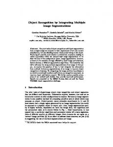
Much research in computer vision has gone towards finding sets of features that are sufficient to perform specific tasks.The result has been a number of systems that work well in their own specific domains, but are not extendable to other domains. Clearly, a general feature set that would be good for most object recognition tasks is desirable. However, recent research in the automatic generation of object recognition programs has demonstrated that pre-determined, 6xed feature sets are often incapable of providing enough information to unambiguously determine object identity and pose. Given any set of features, it is possible to specify a set of objects for which the feature set is insufficient and will result in ambiguity. One approach to overcoming the problem of insufficient feature sets is to utilize multiple sensor observations obtained from different viewpoints, and combine this information with knowledge of the 3D structure of the objects in order to perform unambiguous object recognition. By making use of observations from multiple viewpoints, two objects that have several poses which are indistinguishable can still be recognized as long as there is a distinguishing pattern of observations for each object. As a simple example, the front ends of a sedan and a station wagon may be indistinguishable,but the side views are not. For complex sets of objects, more than a single additional observation may be required to resolve ambiguity - in fact, it is possible that a pair of objects could differ only in the sequence of observations, rather than in the value of any given observation. Consequently, multiple observations should not be made at random, but should be planned out, based on knowledge of the objects and on the basis of the observations already made. The purpose of the research described in this report is to explore the multiple observation strategy for objcct recognition. To contrast this with other object recognition research, consider a graphical representation of recognition stmtegies. as in Figure 1. The x-axis represcnts the size and complexity of the feature set, and thc y-axis rcprcsents the number of observations used. Most current computer vision research is focused on the single linc rcprcscnting obscrvation strategies employing a single observation. There is an enure space of strategies left to explore. In this research, we are beginning to explore the region near the y-axis; that is, we employ relatively small. simple feature sets, but rely on multiple observations. From a practical point of view, our research can be thought of as exploring means of using multiple observations from different viewpoints to increase the information available from cheap. simple, sen-
sors. This report is structured as follows. The next section is an overview of objcct recognition and rclatcd work. In scction 3, we restrict ourselves to the case in which the sensor and object each have a single degree of frecdom, and examine the data structures and planning techniques necessary to utilize multiple observations. Section 4 discusses extensions of the restricted techniques to higher degrees of freedom. in section 5. we present the results of applying multiplc observations to the problem of object localization in the single degree of freedom case. Both simulatcd and real experiments were performed, and the results are demonstrated in several application domains. Finally, in the last scction, we discuss the significance of our approach, and our plans for future research.
3
number of
obseNations+
I
computer vision research
feawe%t size and complexity
Figure 1: The Space of Object Recognition Strategies
4
2 Background and Related Research There are two areas of research leading up to the work reported here. The first area of research is that of planning for sensor observations. The second arm is that of automatic compilation of vision programs. Each of the a r e s is discussed below.
Planning of Sensor Operations The early work in planning ofsensor observations wete only concerned with single observations. That is, the question addressed was that of determining the optimal sensor and light source position to obtain the best image. As tasks became more complex, and the number and similarityof objects increased, the need for multiple observations became apparent. The work of Cowan and Kovesi [6]examined the problem of automaticallygenerating the collection of possible camera locations given a set of sensing requirements. Their approach made use of explicit models of both the object and the camera, and solutions satisfied requirements of spatial resolution, focus, and visibility. Their approach converts each requirement into a geometric constrainr Each requirement defines a region of three-dimensional space that satisfies the requirement, and the intersection of the regions is the set of solutions. Yi et al[25] devised an optimization approach to determine the location of both the sensor and light source to obtain the best image. Their approach was based in terms of edge visibility; they considered both geomctric visibility, which specifies how much of an edge is visible (not occluded), and photometric visibility, which specifies how much of the edge has sufficient contrast to be detectable. Assuming a fixed distance from object to sensor, the vicwing sphere is uniformly sampled, and at each sample, measures of both geometric and photometric edge visibility are computed. A given vision task may be optimized in one of two ways: either maximizing the number of edges visible in an image, or making as much of a given edge visible as possible. Optimality criteria for each condition were determined. Goldberg and Mason [ 101 investigated the problem of determining optimal sequences of squecze grasp operations for determining object pose. They applied the Bayesian framework to the problem. Assuming a uniform distribution of initial poses and a frictionlessparallel-jaw gripper, they demonstrated a program for automatic planning of sequenccs of grasps that optimize the robots expected throughput. Particularly notable is their use of the object diameter function. For polygonal objects, the diameter function is piecewise sinusoidal, but during a squeeze, the object routcs to reduce the diameter, terminating in a local minimum. Thus, a grasping operation not only reduces uncertainty, but converts the diameter function into a piecewise constant function which is more easily analyzed. Since the goal was optimal plans, they used breadth-first search to expand the state space. In the domain of learning robots, Ming Tan [23] addressed the problem of learning sensing strategies. His system, CSL, was implemented on a real robot, and emphasized learning of minimum cost, robust sensing strategies. Given a basic knowledge of moving. sensing, and grasping procedures (cost, preconditions, features, and expectcd errors) and a set of mining 9 objects labeled by their grasping procedures, CSL directed a robot to interact with the objccts and build up a set of procedures for object recognition and grasping while minimizing the expected cost. Maver and Bajcsy [181 investigated the problem of describing a random arrangement of unknown objects in a scene, rather than identifying a known object. They used a laser scanning system which measures nnge 10 visible points. Occluded regions were modeled as polygons. Based on the height information and the geometry of the edges of the polygonal approximation, the next best view is determined. Liu and Tsai [17] used multiple 2D camera views to recognize 3D objects. Recognition is performed by matching 2D silhouette shape features against model features taken from a set of fixed camera views. The systcm made use of two cameras and a turntable for translation and rotation. Their system first reduces ambiguity by taking images from above the turntable to normalize the top-view shape, position the object centroid, and align the objcct principle axis. Next, a side view is taken, and the features analyzed. Until recognition is accomplished, the object is then rotated by 4 5 O , and a new image acquired and analyzed.
5 Hutchinson and Kak [14] demonstrated a system for dynamically planning sensing strategies, based on the current best estimate of the world. Given a work cell with welldefined sensing capabilities, their approach is to automatically propose a sensing operation, and then to determine the maximum ambiguity which might remain if that operation were applied. The system then selects the operation which minimizes the remaining ambiguity. Dempster-Shafer theory [22] was used to combine evidence and analyze proposed operations.
Safranek, et al[20] addressed the problem of combining low-level measurements, each of which is uncertain, in order to verify the location of an object. They showed that the combination could be achieved via Dempster-Shafer theory using binary frames of discernment They showed that, with huge amounts of data, belief functions can become saturated, leading to erroneous conclusions that cannot be altered by additional data
2.1 Automatic Compilation of Vision Programs 'Qpically. a computer vision system is essentially a custom solution to a specific problem, and is therefore expensive to develop and install, and is capable of recognizing only a single part of a smaU number of parts under very special conditions. Modifications to existing systems are difficult to make. Moreover, there is little transfer from one system to another, and so each new system costs as much to develop as the first system did. Recently, work in the area of automatic recognition program generation has addressed the problem of cost-effective system development. A new paradigm, appearance-bused vision [ll]. formalizes and automates the design process. Appearance-based vision can be characterizedas an automated process of analyzing the appearances of objects under specified observation condition, followed by the automatic generation of model-based object recognition programs based on the preceding analysis. An appearance-based system is known as a Vision Algorithm Compiler, or VAC. A VAC is highly modular. Both objects and sensors are explicitly modeled, and are therefore exchangeable. Hence, a VAC can generate object recognition code for many different objects using the same sensor model, or the set of objects can be fixed and h e sensor models varied.
A VAC incorporates a two stage approach to object recognition. The first stage is executed off-line and consists of analysis of predicted object appearances and the generation of object recognition code. the second stage is executed on-line. and consists of applying the previously generated code to input images. The first stage is executed only once for a given object recognition task. and can be relatively expensive. The second stage is executcd many times, and must be both fast and cost-effective.The high cost of the first stage is amortized over a large number of executions of the second stage.
Goad [9] presented one of the first programs capable of automatically constructing an object recognition program. In Goad's system. an object is described by a list of edges and a set of visibility conditions for each edge. Visibility is determined by checking visibility at a representative number of viewpoints obtained by tesscllating the viewing sphere. Object recognition is performed by a process of iteratively matching object and image edgcs until cither a satisfactory match is found, or the algorithm fails. The sequence of matchings is compiled during the off-line analysis phase. Goad's system was not completely automatic, however. Goad selected edges as the features io be used for recognition, and the order of edge matching was specified by hand. The 3DPO system of Bolles and Horaud [31 was built with the intended goal of using off-line analysis to produce the fastest, most efficient on-line object recognition program possible. 3DPO utilized the local-fenture-focusmethod, in which a prominentfocus feature is initially identified, and then secondary features predicted from the focus feature are used to fine-tune the localization rcsult. The system was not fully automatic, as the focus features and secondary features were chosen by hand. Ikeuchi and Kanade [15] first pointed out the importance of modeling sensors as well as objccts in order to predict appearances, and noted that the features that are useful for recognition depend on the sensor being used. Their systcm predicts object appearances at a representative set of viewpoints obtained by tessellating the viewing sphere. The
6
appearances are grouped into equivalence classes with respect to the visible features; the equivalence classes are called uspects. A recognition strategy is generated from the aspects and their predicted feature values, and is represented as an interpretation tree. Each interpretation tree specifies the sequence of operations rcquired to preciscly localize an object. The sequence of operations is broken up into two parts: the first part classifies an input image into an instance of one of the aspects, while the second part determines the precise pose (position and oricnution) of the object within the specified aspects is broken up into two parts: the first part classifies an input image into an instance of one of the aspects,while the second part determines the precise pose (position and orientation) of the object within the specified aspect. Hansen and Henderson [121 demonstrated a system that analyzed 3D geometric properties of objects and generated a recognition strategy. The system was developed to make use of a range Sensor for recognition. The system examines object appearances at a representative set of viewpoints obtained by tessellating the viewing sphere. Geometric features at each viewpoint are examined, and the pmperties of robustness, completeness, consistency. cost, and uniqueness are evaluated in order to select a complete and consistent set of features. For each model, a strategy tree is consaucted. which describes the search shategy used to recognize and localize objects in a scene.
The system of Arman and Agganval [I] was designed to be capable of selecting the proper sensor for a given task. Starting with a CAD model of an object, the system builds up a tree in which the root node represents the object, and the leaves represent features (where features are dependent upon the sensor selected), and a path from the mot to a leaf passes through nodes representing increasing specificity.Each arc in the tree is weighted by a “reward potential” that represents the likely gain from traversing that link. At run time, the system traverses the tree from the mot to the leaves, choosing the branch with the highest weight at each level, and backtracking when necessary. The PREMIO system of Camps, et a1 [5] predicts object appearances under various conditions of lighting, viewpoint, sensor, and image processing operators. Unlike other systems, PREMIO also evaluates the utility of each feature by analyzing the detectability. reliability, and accuracy. The predictions are then used by a probabilistic matching algorithm that performs the on-line process of identification and localization. The BONSAI system of Flynn and Jain [7] identifies and localizes 3D objects in range images by comparing relational graphs extracted from CAD models to relational graphs constructed from range image segrncntation. The system constructs the relational graphs off-line using two techniques: first, view-independent features are calculatcd directly from a CAD model; second, synthetic images are constructed for a representative set of viewpoints obtained by tessellating the viewing sphere, and the predicted areas of patches are determined and stored as an attribute of the appropriate relational graph node. During the on-line recognition phase, an interpretation tree is conslructcd which represents all possible matchings of the graph constructed from a range image, and the stored modcl graph. Rccognition is performed by heuristic search of the interpretation tree.
Sam, et a1 1191 demonstrated a system for recognition of specularobjects. During an off-line phase, the system generates synthetic images from a representative set of viewpoints. Specularities are extracted from each image, and the images are grouped into aspects according to shared specularities, and each specularity is cvaluatcd in tcrms of its detectability and reliability. A deformable template is also prepared for each aspect. At execution time, an input image is classified into a few possible aspects using a continuous classification procedure bascd on Dcmpster-Shafcr theory. Final verification and localization is performed using deformable template matching.
2.2 The Need for Resolution Hong, et al 1131 extended the work of Ikeuchi and Kanade by optimizing the object recognition code generated by their VAC. They noted that, in many instances, objects have aspects that cannot be distinguished on the basis of available features. They called these aspects congruenf uspects. Since congruent aspects form equivalcnce classes with respect m a feature set, they are grouped into larger sets called congruenr cfusses.The linear shape change dctermination process can sometimes overcome the ambiguity in aspects, but not always, and only at greatly increascd computational cost.
7
Congruent aspects appear to be a universally encountered, if not generally recognized phenomenon of objcct recognition systems. In the work of Hong et al, most of the objects for which recognition programs were gcncratcd exhibited congruent aspects. More recently, Siebert and Waxman 1211 reported an adaptive object recognition program and noted that 75% of the aspects generated by their system were ambiguous. In human-dcsigned systcms, congrucnt aspects exist, but are not noted; the vision system designer is specifically engaged in looking for a feature sct hat will not be ambiguous, and is therefore not likely to notice the phenomenon as anything more that a failure of a specific feature set. However, we speculate that the congruent aspect effect is responsible for the fact that virtually every object recognition system uses a unique feature set A little thought shows that, for any given feature set, there exist objects which have congruent aspects with respect to that feature set. Additionally, factors such as sensor noise and occlusion can reduce the sensitivity of a feature set and add to ambiguity; in effect, these factors create congruent aspects. Given that congruent aspects cannot be avoided, how can they be handled? The typical approach, that followed by most vision system designers, is simply to keep developing new feature sets. That is. when the current feature set fails, resulting in congruent aspects, a new feahm set is developed that is specialized for that object domain. Another approach that has received less attention, is to utilize multiple observations from different viewpoints, using knowledge of the 3D shape and sensor positions to combine information from different observations.
8
3 Planning Multiple Observations In the most general case of planning multiple observations, multiple objects would be considered, each of which would have six degrees of freedom in pose, and the sensor involved would also have six degrees of frcedom. The resulting planning space would then be 12 dimensional. Gaining any intuition in a 12 dimensional space would be difficult, and the details of representation and bookkeeping would likely obscure any generalizations. Therefore, to gain insight into the problem, we restrict our aaention initially to the simplest case, that in which the sensor and the object each have one degree of freedom. In the next section, we build on that base and extend the planning methodology to the case of three degrees of freedom in object and sensor. Additional extensions to still more general cases are possible.
To start off, we consider the case in which the distance to the object remains fixed, the object has one axis with known orientation about which it can rotate,and the Sensor is constrained to rotate in a plane about the object perpendicular to the h o w n object axis. Hence, there is a single degree of freedomeach in sensor motion and object pose; since sensor and object rotate about the Same axis, the system as a whole still has only one degree of freedom. Figure 2 illustrates this case.
Figure 2: Object Recognition with One Degree of Freedom
The one degree of freedom case described above is simple, but still similar to a variety of application domains. One example scenario is that in which a mobile robot moves around an object in order to recognize it - the robot motion is locally planar, the distance to the object remains fixed, and in many cases,such as automobiles and furniture, objects have a known “upright” posture. Another application scenario is that of sensing the pose of an object from measurements of object diameter made by tentatively grasping the object from above and measuring the gap between the manipulator fingers: we call thisfinger gap sensing, and demonstrate planning in this domain in section 5. As stated in the previous section, an aspect represents a characteristic view of an object. Intuitively, an aspcct corresponds to a contiguous set of viewpoints from which the object looks “more-or-less the same”. Aspect classification is the process of classifying an input image into an instance of an aspect Aspect classification is essentially a process of rough localization, since it limits the possible object poses to those consistent with the obscrved aspect. For many tasks, the rough localization determined by aspect classification is sufficient. In what follows, we assume that this is
9 the case, and consider the problem of localization to be equivalent to that of determining the aspect oriented in a particular direction. For example, to grasp an object stably with a parallel jaw gripper, it is only necessary to align a particular aspect of an object with a reference point of the gripper. given such an alignment, the object is guaranteed to slide into position when contacted by the gripper [4]. In a computer vision system, aspects can be defined in a variety of ways. For example, aspects can be based on the set of visible object surfaces, or on the range of a specificfeature. Aspects can be characterizedby determining the distribution of feature values over all the viewpoints within each aspect. 4spects with feature distributions that cannot be distinguished are congruent. We refer to a set of congruent aspects as an aspect class. Figure 3 illustrates a simple example. Suppose that the shape at the top is the projection of a solid 3D object which is to be viewed from within the plane of the page, and assume orthographic projection. Aspects of the object have been defined based on the set of visible surfaces. Numbering surfaces counter-clockwise from the right side. aspect 0 is defined by the set of viewpoints for which surfaces 0 and 1 are visible. For aspect 1, surfaces 0, 1, and 2 are visible. For aspect 2. surfaces 1 and 2 are visible. The rest of the aspects are d e w by noting where surfaces appear and disappear. Now. assuming that the area of each surfax is the only available feature, then surfaces 1 and 4 are indistinguishable, as are surfaces 2 and 3. The resulting aspect classes are labeled in the figure. , Clearly, if the feature distributions of two aspects cannot be distinguished, then additional sensor observations from the same viewpoint will contribute nothing to the problem of distinguishing between the aspects. However, the problem changes when Sensor movement is allowed. Unless an object is perfectly symmetrical, the relative position of other aspects will be different for different aspects. In principle, then, two congruent aspects can be distinguished by moving the sensor to another location from which different observations will result, depending on the identity of the original aspect. We call this process aspect resolution, and refer to the distinguishing observation as a resolving observation.For nearly symmerhcal objects, it may take more than one sensor move and obscrvation to rcsolve congruent aspects: instead, it may require a long Sequence of sensor moves and observations, referred to as a resolving sequence.
To make these definitions intuitive, consider again the example illustrated in Figure 3. The object in question has four congruent aspect classes. The first observation is of class-I, which limits the possible object poses to those corresponding to either of aspect-1 or aspect-6, shown shaded at the bottom of the figure. The second observation, taken 45' from the first, is of class-0. The combination of class-1 followed after 45' by class4 limits the object pose to the set shown shaded in the figure: that is, it is now known that the object is positioned in such a way lhnt aspcct-6 was initially visible In this case, aspect resolution has restricted the object's pose to be one consistent wilh an initial observation of aspectd. The example shown in Figure 3 is fairly simple, and it is easy for a human observer to determine one or more resolving moves for any of the aspect classes. In fact, for many three-dimensional cases, the determination of resolving moves is relatively easy for a human to perform. However, the problem is not immediately solvable automatically. Several key issues have to be addressed to automate planning for aspect resolution. These issues includc the following: object representation The object must be represented internally in such a way as to make explicit such object propertics as the geometric extents of and relations between observation classes. For example, in Figure 3, the rcquisite knowledge included the facts that both aspect-1 and apect-6 spanned 45' and belonged to the same congruent aspect class. Furthermore, it was necessary to know the extents and classes of all the other aspects of the object.
representation of uncertainty A given observation may not constrain the pose of the object by much, and so it is not possible to move to particular positions in order to perform observations. For example, in figure 1, the first observation only constrained the object pose to within two sets, spanning a total of 90'. and any motion of less than 45' would not be guaranteed to provide useful information. Moreover, even after resolution, the uncertainty
.
10
aspect-1 class-1
aspect-2 class-2
I
class-2
0class- 1
class-0
6 X
observation 1
observed class
possible poses
observation 2
Figure 3: Resolution of Congruent Aspects was only reduced to a set spanning 45". Therefore, every move must be made with respect to the current uncertainty in position. The internal representation used to plan moves must explicitly represent uncertainty in position. selection of moves There are an infinite number of moves that can be made from any location. It is clearly impossible to search through all moves to select the best. A system for planning resolving moves must have some consistent means of selecting potential moves from the infinite number of possibilities. Each of the issues above is addressed in the sections below.
3.1 Object Representation Aspects were originally defined in [161 as topologically equivalent classes of object appcaranccs. More intuitivcly, an
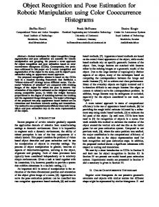
aspect can be considered to be a continuous collection of viewpoints yielding object appearances that all look the same. An example is illustrated in Figure 4, in which only equatorial aspects are considered. In the figure, aspects are defined by the set of visible faces. Note that if only geometric, and not relational, information is considcrcd, then there are 4 sets of congruent aspects: (1.81. (2.71, (3.61, and ( 4 5 ) .
3d object
equatorial aspects
aspect appearances
mmm
Figure 4: Equatorial Aspects for Polyhedral Solid, hexubj
In our domain, the important information about an object that must be made explicit in the object rnodcl includes: the geometric extent of each aspect, geometric relations between asp&ts, and descriptions of aspects in terms of feature values. Since our domain is only two dimensional, rather than employ the full aspect graph, as prcscntcd in [ 161, we represent the information in the form of an aspect diugrum. The aspect diagram is like a pie chart; it divides the vicwing circle up into pie-shaped wedges, each wedge representing an aspect. The extent of each aspect is rcprcscntcd by the size of the wedge, and relations between aspects can be computed directly from extcnt and ordcring information. Each aspect can be characterized in terms of the feature values associated with it. That is, a singlc vicw of an object can be described in terms of the features extracted from that view. An aspect can then be characterized by the range of features values extracted from the constituent views of the aspect The range of values can either bc computcd analytically, using object and sensor models. or can be approximated by sampling appearances at sclcctcd vicwpoints. Given the ranges of feature values for an aspect, there is a straightforward procedure to gencratc an aspcct classification program. Starting with the set of all aspects, each feature is examined to see if the sct can bc partitioned on the basis of the values of that feature. Each resulting subset is then tested against the remaining fmturcs, and the proccdure is iterated until either each aspect is uniquely determined, or no more features can be applied. The non-singlcton aspect sets remaining at the end of the process are congruent aspect sets, since they cannot be distinguishcd using thc available features. The congruent aspect sets define the aspect classes. Figure 5 illustrates the aspcct diagram corrcsponding to the object and aspects from Figure 4. The diagram clearly depicts the extent, relativc location, and class of each aspect.
12
Figure 5: Aspect Diagram for Equatorial Aspects of Hexobj
3.2 Representation for Planning 3.2.1 The Observation Function and Observation Graph Let yobe a position on the viewing circle around an object. We can define an observation function that relates the angular displacement from voto the observed aspect class with respect to the object coordinate system:
where Y denotes the set of relative viewing positions. and r = (y1 ...yn) denotes the set of aspect classes. For example, for the aspect diagram of Figure 5 , the following equalities hold: R (0') = class-0, and Q ( 120' ) = class-3 . Pictorially, we can illustrate the observation function for the aspect graph of Figure 5 as the one-dimensional labclcd line segment shown in Figure 6. The graph extends infinitely to both sides, and is pcriodic modulo 2rr. c-01 c-1
I c-2 I
c-3
I
c-4 I c-4
I
c-3
I c-2 I c-1 I c-0
I 0'
180'
360'
Figure 6: Graph of Observation Function
Note that the observation function defined above, and illustrated in the figure, depends on knowing thc objcct coordinate system, and specifying displacements with respect to that coordinate system. In object localization problems, one of the goals is to determine the object coordinate system. In the case being considcrcd hcre, h e rclationship between object and world coordinatescan be specified by a single parameter, 8, which is the angular displuccmcnt of the object from its base position. Alternatively, 8 can be regarded as the relative rotation bctwccn object and scnsor. The graph of the observation function illustrated in Figure 6 is for a value of 8 = 0. The graph of thc function for 8 = 30' would be the graph of Figure 6 shifted 30' to the left.
Thus, for a known displacement of world to object coordinates, the observation function is onc-dimcnsional, and
13 reflects the fact that perfect positional information can be used to accurately predict the results of sensor observations. However, perfect positional information is rarely, if ever, known. In particular, the object pose is never known exactly at the start of an object localization task. Hence, we need a way to include uncertainty in the object pose into the observation function: this can be done by adding an extra dimension to the observation function. The general observation function for the one degree-of-freedomrecognition problem therefore becomes:
n: ( w e + r )
(2)
where Y and I' are defined as in (1). and 8 denotes the set of possible object poses. Hence, the expression Q(yr.0) denotes the aspect class observed by moving the Sensor w degrees with respect to the origin of the object coordinate system rotated 9 degrees from world coordinates. The graph of the observation function is now two-dimensional,and we refer to it as the observation graph. The observation graph correspondingto the object in Figure 4 is illustrated in Figure 7 for 0'I y~,9 < 360'.
-
t Key:
w
CI~SS-o
class-1
class-2
F I r-l
class3
class4
........... ............ ............. ........... ............... ............ ..........................
Figure 7: Observation Graph for Hexobj for 0' I y~,9 < 360'
Any horizontal line drawn through the figure would yield the observation graph for the object in a particular pose. For example, horizontal lines drawn through the top and bottom of the figure would be identical to the graph in Figure 6,
14
which is the observation graph for the object at its base position. The vertical axis represents uncertainty in object pose. For example, any position on the \~raxis represents a sensor position. The vertical line through that position rcpresents the ordering of the set of possible observations as a function of object pose. Thus, if the object pose was known to within 30°,and the sensor was at a known position. then the vertical line segment at the sensor position extending 30" above and below the approximate pose would represent the set of possible observations rcsulting from that uncertainty in pose. Let the resolutionfunction that maps sensor position and object pose onto (sensed) aspect identity be denoted:
a:( Y x e + A )
(3) where A = (al, ...&) denote the aspects of an object. Given a sensor position and an object pose. the resolution function identifies the underlying aspect. The output of the process of aspect resolution is exactly the value @(Oo, 9). where 8 is the pose of the object. hence the name given to the function 0. The observation function can be restricted in various ways to define observation functions for various subsets of w and 9. The aspect-restricted observation function is defined by:
Graphically, an aspect-restrictedobservation function is represented by a single horizontal strip in the region 0 I 9 < 2x that is periodic modulo 2x. The width of the strip corresponds to the width of the defining aspcct. Intuitively. the aspect-restricted observation function Ra,represents the collection of observations that could result if aiwas the aspect underlying the first observation. Th'e aspect-restrictedobservation function represents the situation that results when a particular aspect has been identilicd. but the exact pose of the object is unknown. The results of additional observations can be predicted to within an uncertainty defined by the size of the aspect Similarly. the class-restricted Observation function is defined by:
The class-restricted observation function R, represents the collection of observations that could result if the initial observation was of class 3.A class-rescrictddobservation function can be represented graphically as a collection of horizontal strips in the region 0 < 8 < 27t that is periodic modulo 2x. The number of strips in each period is exactly the number of aspects belonging to class yj, and the width of each smp corresponds to the widlh of the defining aspect. The class-restricted observation function represents the situation that results when a particular aspect class has bccn observed, but the particular aspect is unknown. In this case,the results of additional observations can be predicted to within an uncertainty defined by the sizes of the constituent aspects. In summary, then, the observation function is a representation of the relationship of object pose and sensor position to sensor observation. The observation graph is a pictorial representation of the observation function, in which the horizontal axis represents sensor position. and the vertical axis represents object pose. A horizonul line through the observation graph represents the variation in sensor observations that would result from Sensor motion rclative to a particular object pose. A vertical line through the observation graph represents the variation in scnsor obscrvations that would result from object rotation relative to a particular sensor position.The aspect-restricted obscrvation function represents the uncertainty in sensor observations when the sensor is moved with respect to thc observation of a particular aspect. The class-reslrictedobservation function represents the uncertainty in sensor observations when the sensor is moved with respect to the observation of a particular aspect class.
3.2.2 Aspect Resolution and the Observation Function In what follows, we will cease to worry about the periodicity of the observation function and concern ourselves with the primary interval for which 0 < y,8 < 2x. It is convenient to use modulo arithmetic and consider the Observation
15
function to exhibit wrap around. The goal of object localization in our restricted domain is to determine the exact value of eo. the orientation of the object with respect to world coordinates. Mathematically, object localization restricts the observation function to the one-dimensional function R(y,00). Equivalently, object localization is the restriction of the obscrvation graph to a single horizontal line corresponding to R(y, 00). The goal of aspect resolution is less ambitious than that of object localization. Rather than determining an exact value of 80, aspect resolution determines a range of orientations (&, &,) and an aspect ai,such that aspect q is guaranteed to underlie any observation in the interval; mathematically,V f k (e&,), 3! i 3 a(0.e) = q.Equivalently, object localization is the restriction of the observation graph to a horizontal strip that is a subset of the strip defining the aspectrestricted observation function. The tool which can be applied to perform aspect resolution is a sensor observation, which yields the class of the underlying aspect. Since an observation yields only class information, a single observation reduces the observation function to some class-restricted observation function. If no congruent aspects are present. then each class contains only a single aspect, so the class-restrictedobservation function is equivalent to an aspect-restrictedobservation function, and the task is completed. More generally, however, in the presence of congruent aspects the class-restricted observation function is equivalent to the union of the aspect-restricted observation functions corresponding to the aspects making up the class. Graphically, an observation reduces the observation graph to one or more horizontal strips.
To formalize this concept somewhat. define the observution-restrictedobservation function by:
Intuitively. the observation-restrictedobservation function is the subset of the observation function that is consistent with a particular observation.For example, if an observation made with a sensor displacement of yo yicldcd an observation of uj, then the restriction of the observation function consistent with this observation would be dcfincd only for 8 for which R(yo.0) = Figure 8 illustrates a restriction of the observation graph of Figure 7 for the obscrvation R(90',e) = class-3. This observation-restricted function corresponds to a subset of the union of the aspcct-restrictcd functions q s P e C t - 5QSPectd. zzIspect-a. and Raspect-o.
x.
Each observation restricts the observation function to a subset that is consistent with that observation. If the relationships between multiple observations are known, then multiple restrictions can be applied to the obscrvation function. Graphically, the operation is that of intersecting the strips resulting from the individual operations. Whcn the multiple restrictions result in a subset of the aspect-restricted observation function for a single aspect, thcn aspcct resolution has been completed. For example, the observation of n(90*,e) = class3 results in the obscrvation-rcsuictcd obscrvation graph of Figure 8. A second observation of R(210', e) = class-0 would result in a single horizonml suip which would correspond to the union of the two aspect-restrictedfunctions QSPect-5and qspect-6. The two obscrvations at 90' and 210' thus fail to resolve the aspects and another observation is needed. Instead of 210'. a bcttcr position for a second observation is 300'; then, whatever class is observed provides sufficient information to resolve thc aspects: an R(300', 0) = observation of R(30'. 0) = class-2 yields a subset of the aspect-restricted observation function RJspecl-6; class-3 yields qsPect-5; R(300'. e) = class-1 yields QSpea-o; R(300'. e) = class-0 yields l&specl-3. A procedure for using the observation function to perform aspect resolution now suggests itselk conslruct t k obscrmtionfvnctwn for the object perform a sensing operation
construct t k obsermtion-restrictedobscrmticnfunction corresponding to t k obscrmiion while (the observation-restriction is not a subset of any aspect-restriction)do select a new sensor posirion and m e 1k sensor perform a sensing operation construct a new observation-restriction by updating tht old
done
16
w Key:
CI~SS-o
class-1
r i
class-2
w
class3
class4
............. ........... ......................... ............... .................. .
Figure 8: Observation Graph for Hexobj Restricted to !2(90",0) = class-3 The key problems that yet remain are: How can the observation graph be used for planning aspect resolution? How should new sensor positions be selected? These problems are addressed in the next subsection.
3.3 Planning with the Observation Graph Thus far, we have shown that any given feature set will exhibit a phenomenon known as congruent aspects. Congruent aspects are distinct aspects with indistinguishable feature sets and hence belong to the same aspect class. Aspect resolution is the processing of disambiguating congruent aspects so that the particular aspect originally obscrvcd is known uniquely. Aspect resolution can be performed relatively simply by moving the sensor to differentpositions and kccping track of the observations. The pattern and displacementsof the observations can provide sufficient information to disambiguate congruent aspects. The problem then becomes one of picking the positions of subsequent obscrvations and combining the information properly. The problem is complicated by the fact that the exact position of the sensor with respect to the object is never known exactly. Instead, a range of possible positions is known. The observation function is a representation that relates uncertainty in object pose and scnsor position to sensor observations. In particular, restrictions of the observation function can be consuuctcd to yicld the exact pattern of sensor observations with respect to particular aspects, classes, or even individual observations. Using the observation function, it is possible to predict, with known uncertainty, the range of possible observations that might result from a sensor operation executed at a particular position. The observation function therefore provides all the information needed to plan moves to perform aspect resolution.
17 However, the observation function is a mathematical construct which must be made more concrete before bcing usable. A more useful form of the observation function is the observation graph, which is a two-dimensional, graphical representation of the observation function. The previous subsection showed several examples of observation graphs. This section will show how to use observation graphs to plan resolving sequences of sensor moves. We assume that the first observation defines the 0' sensor position, so all moves will be madc with respect to this position. The outcome of the first observation is a restriction of the observation graph to be consistent with the observed class. Figure 9 illustrates the restriction that is consistent with an initial observation of class-3.
"T aspect-6
aspect-3
Key:
CI~SS-O
class-1
class-2
clu-3
class-4
Figure 9: Observation Graph for Hexobi Restricted to Q(O',O) = class-3
Each observation made results in an additional restriction of the observation graph. What is nccded, thcn, is a way to select sensor positions. or moves. in such a way as to result in a useful restriction. The problcm is that thcrc is potcntially an infinite number of moves. An examination of the structure of observation graphs simplifies the move selection problcm. Thc obscrvation function is discontinuous, with the discontinuities occurring at the boundaries between diffcrcnt obscrvation results. These boundaries are linear, and span the extent of the observation graphs, and therefore span any rcstrictions.Let thc points along the border of restricted observation graphs at which the obscrvation function is discontinuousbc rcfcrrcd to as nodal points. Nodal points can be ordered with respect to their w coordinates. Considcr an obscrvation graph G , wilh nodal points n1 < n2 c... c np. The linear structure of the observation graph guarantees that, for any pair of adj:icent nodal points n; and ni+lr the set of observations (Q(y.0)) possible is the same for any w such that n; c w c ni+l Graphically, this means that any vertical line through the observation graph between adjacent nodal points will intersect the same regions; only the relative extent of the portion of the regions underlying the lines will vary. Since the information between nodal points is constant, only nodal points need be considcred when sclecting sensor moves. Thus, an infinite number of moves has been condensed down into a finite. although possibly large, set of moves. Each distinct nodal point represents a possible sensor move. Each observation possible for a givcn move spccices a restriction of the observation graph. Each such restriction can be examined to see if it results in aspcct resolution. Additional moves can be examined by examining the observations possible at the new nodal poinw rcsulting ' from each new restriction. Figure 10 illustrates the procedure on hexobj for moves at 180' and 240'. As sccn in the figure, the move at 180' fails to resolve the aspects; either of the two possible observations can result starting from
18
either aspect. The move at 240'. however, does result in aspect resolution.
R(v, e) = class-3 n
n(i8o*, e) = cia~s-2
e+ n(o*,e) = class-3
II
/\ \
R(240': b) = cla~s-0 [
R(V. 0) = class-3
I
Figure 10: Two Possible Moves Following R(WJ3) = chss-3
While Figure 10 depicts only two of the possible moves starting from Q(V. e) = class-3, it illustrates thc tree suucture of the collection of possible move sequences. We call this tree the observation tree. Starting from any obscrvation graph, there exists a set of moves dcfincd by the nodal points of the graph. Each of these moves can rcsult in I limited number of observations, each of which gives rise to a new, more restrictcd, observation graph. Each new observation graph has an assochted set of nodal points that define the moves that lead to furthcr rcstrictions, and so on, recursively. Since the objective of using multiple observations is to perform aspect resolution. the branching process can be terminated at any restriction which is resolved. Hence, leaf nodes reprcsent the rcsolution of somc aspcct.
19
Some sequences of moves never result in aspect resolution, and the branching process for the subtrees representing these sequences never terminate. Planning for aspect resolution consists of searching through the observation tree,looking For subtrees in which every aspect is resolved. We call such a subtree a resolving subtree: one test for a resolving subuee is to verify that the collection of resmcted observation graphs at the leaf nodes covers the observation graph at the root. In practice, despite the use of nodal points to define moves, there are many possible moves at every node of the observation tree. As a result, there are many possible resolving subtrees- many more than are practical to enumerate. Additionally, For complicatedobjects (as will be seen in section 5). aspect resolution may require several observations: five or six observations are not unexpected. The result of all this is that observation trees are far too large to search exhaustively, so heuristic search is required. The resolving subtree that results from search of the observation tree is called a resolution tree, since it specifies a sequence of moves that will perform resolution for any aspect. The resolution tree becomes a specification for an online executive that performs observations until aspect resolution is complete. In many cases, the resolution tree is quite simple, and contains only a single move level. For example, Figure 11 illustrates the aspect diagram and the corresponding resolution tree for hexobj.The resolution tree shown has three types of nodes. Move nodes, represented by
b
Figure 11: Aspect Diagram and Resolution Tree for Hexobj circles and labeled with “M-”, denote sensor moves: the move position is indicated in degrees. For example, the root node is a move node labeled “M-0”. and the sensor position is 0’.All moves are relative to the initial .position. Condenote sets of congruent aspects. The observed class is gruent-set nodes, represented by squares and labeled “C-”, indicated within the square, as well as the labels of the congruent aspects. Resolved nodes. also represented by squares but labeled “R-”,denote aspects that have been resolved. The leftmost descendant of the root node is a resolved node: the observation resolving the aspect is class-2, and the resolved aspect is aspect-2. The two rightmost descendants of the mot node are congruent set nodes. The rightmost node represents the case that occurs from an observation of class-0. which yields the congruent aspects aspect-0 and aspect-4. Note that all lcaf nodes are rcsolvcd nodes. The resolution tree provides directions for resolving congruent aspects. Thus, in the figure, thc first action is an obscrvation made from the initial position, 0’.If the observation is class-0, then the aspect observd is aspect-0. The node is a leaf node, so the aspect has been resolved and processing terminates. If the first Observation is of class-2, then either of aspect-2 or aspect-7 could be the initial aspect. A move of 330’ should be made. If the resulting obscrvation is class-1, then the initial aspect was aspect-2; if the resulting observation is class-3, lhen the initial aspect was aspcct-
.
20
7. Figure 12 illustrates another, somewhat more complicated example, in which two moves may be necessary to resolve a set of congruent aspects. The examples in the section on experiments show still more complicatcd cases in which as many as seven observations are required to resolve some aspects. mi2
m --2 C
l
-4 c i a 1
d
rCr cl tC- Z3
PD
W - 5
-4 C
l
Cl-I
d
m
Figure 12: Aspect Diagram and Resolution Tree Specifying Two Moves
21
4 Extension to Higher Degrees of Freedom First, we recap the results from the previous section. In the constrained scenario considered there, objects with one degree of freedom in pose were being localized using multiple observations from a sensor with one degrec of freedom in position. In fact, since rotation of the object is equivalent to the inverse rotation of the sensor, there is only one degree of freedom in the system. It was convenient to parameterize the space using two independent variables, however. A two dimensionalobservation function was definedthat mapped object pose and sensor position onto observed aspect class:
n: ( Y X e + r)
(7)
The observation function was shown to have.a representation as a two-dimensional square planar surface. Sensor observations were shown to reduce this square into strips, and planning was performed by examining sequences of sensor positions to find sequences that would yield strips corresponding to subsets of the snips resulting from restricting the observation function to individual aspects. We consider here the extension of planning to three degrees of freedom. Object position is assumed to be known, but the threerotationalparamem defining object pose are allowed to vary. The sensor is assumed to be held a fixed distance h m the object, allowing only the sensor view axis and rotation about that axis free to vary; that yields three degrees of freedom in sensor position. The extension of the observation function and observation graph to three degrees of freedom is similar to the derivation in the single degree of freedom case, the main difference being that the observation graph may take several different forms, all of which are difficult to visualize because of the number of dimensions, and diflicult to work with because of the corresponding sizes of the data structures. The fundamental problem with extending the observation gmph to three degrees of freedom is that rotations around multiple axes are not commutative. As a result, the higherdimensional observation gmph does not have a nice, neat, conceptually simple structure. Moreover, many different representations are possible. For example, pose and position could be described by Euler angles or quaternions, and each description leads to a different representation of the observation graph. Abstractly, there is little difficulty in extending,our previous results. The observation function, Q becomes a scalar function of two vector-valued variables, $ and 8 , which define sensor position and object pose, rcspcctively:
As before, aspect, class, and observation restrictions of the observation function partition the observation function into subfunctions. Equivalently, the higher-dimensional observation graph can be partitioned into disjoint regions corresponding to either aspect-restrictions, class-restrictions, or observation-restrictions. As bcrore, scqucnccs of observationscan be represented as the intersection of the associated restricted observation graphs. Planning for aspcct resolution is again a search through the tree of possible sensor moves to find a subtree in which evcry leaf node is a subset of an aspect restriction. In the sections below, we add some detail to this abstract description by selecting particular rcprescntations and examining the impact of the representationson the aspect resolution planning process.
4.1 P-spheres and O-spheres
’
One representation of orientation that has been found useful in computer vision is the solid Gaussian sphere [ 151, which we will specialize for the representation of sensor position and object pose, and refer to as the position sphere @-sphere) and orientation sphere (o-sphere),respectively. We start by defining the p-sphere.
22 There is a one-to-one correspondencebetween points of the solid unit sphere and sensor positions. First, assume that the object is at the center of the sphere. Then, each point on the surface represents a position of the sensor, with the view axis aligned towards the sphere center. Rotation around the axis can then be represented by distance from the center. The following paragraphs add the details necessary to map sensor positions onto the sphere. Define a sensor coordinate system as shown in Figure 13; the system is left-handed, with the z-axis representing the sensor view axis. The p-sphere is assumed to have an imbedded coordinate system, with the north pole being the intersection of the p-sphere z-axis with the surface of the sphere. Select a home,or base, position for the sensor, and identify this position with the north pole so that the sensor points towards the center of the p-sphere, and the x- and y-axes of the sensor are aligned with the x- and y-axes of the psphere. Points on the surface of the sphere can be identified with orientations of the view axis by rotating the origin of the sensor coordinate system to that point on the surface and pointing the z-axis towards the center of the p-sphere. There is obvious freedom of movement around the view axis, which is eliminated by specifying that the sensor is rotated into position directly from the north pole along a line of longitude. Finally, let distance along the view axis towards the center of the sphere represent rotation clockwise around the view axis. Figure 13 illustrates the definition.
Y
Figure 13: The Position Sphere Representing Sensor Positions
The p-sphere has two singularities: the souh pole, and the center. These singularitiescan be idcntificd in advancc and avoided during the planning process. The same general representation can be applied to the process of representing object pose, in a form that we rcfcr to as the orientation sphere, or o-sphere. We assume that the location of the objcct is known, and that a pose spccifics an orientation relative to some fixed coordinate system. Then, all poses of an object can be dcfincd by three pammetcrs. As above, these parameters can be represented as points on a solid sphere, the o-sphere. Define a coordinate system fixed with respect to the object. Pick one axis of the object, the z-axis, for example, as a distinguished axis of the object. Start with the object coordinate system aligned with the o-sphere coordinate system, and identify this pose with the north pole of the 0-sphere. To specify any pose of the object, first specify the new position of the z-axis; this axis alignment is identified with the ray from the center of the sphere having the same alignment. Next, assume that the z-axis was moved to that position in the most direct way - by movement along a line of longitude. This assumption specifies new orientations for the x-axis and y-axis. Now, let distance from the surfacc toward the o-sphere center represent rotation about the new z-axis. We can represent the observation function as the successiveapplication of two functions: the first is a function-valued function that computes the restriction of the observation function to a single object orientation, and the second is a scalar-valued function that applies the rcstricted observation function to a specific Sensor position and computcs the
23 observation value. More formally:
The intuition behind this formulation is that every point of the o-sphere has an associated p-sphere. Each p-sphere represents the set of possible observations as a function of sensor position for a given object pose. We can labcl each point of each p-sphere with the class and aspect that would be observed by a sensor at the specified position for an object in the associated pose. Thus, to determine the value that would result from an observation of an object in a known pose made from a sensor in a specific position, one accesses the p-sphere associated with the given pose, and then looks up the value at the point of the p-sphere representing the sensor position. The tepresenration described above, that of an o-sphere consisting of pspheres at each point, constitutes the three degree of freedom observation graph. It would also be possible to construct the observation graph by indexing ospheres through a psphere, but certain operations become much more complicated. A continuous implementation of the three degree offreedom observation graph is impractical. Instead, the o-sphere and p-spheresmust be discretized into cells representing ranges of parameters. Each cell of the o-sphere has an associated psphere. or childp-sphere. Similarly, each p-sphere is associated with a specific cell on the o-sphere, which we will refer to as theporent cell. In what follows, we assume that each cell of the o-sphere contains a flag that an be turned on or of, and that each cell of a child p-sphere conrains the class and aspect that would be observed for thc specified pose and position. Initially, all 0-sphere cells are turned on. The three degree of freedom restrictions of the observation graph can now be formulated by selectively turning various cells 08. An aspect-restricted observation graph consists of all the o-sphere cells (and child p-spheres) for which h e specific aspect is observed by the sensor at its base position. Using our representation, we can construct the aspect-restricted observation graph by examining the cells at the north pole of each p-sphere. Each o-sphere cell with thc givcn aspect at the north pole of its child p-sphere is left on, while all others are tagged of. The collection of on cells represents the aspect-restricted observation graph. The class-restricted observation graphs can be similarly conslructcd, by leaving on all o-sphere cells with the correct class at the north pole of the child psphere, and turning all other o-sphere cells off, Construction of the observation-resmcted observation graphs is similar. An observation consists of an ordered pair (f, yi) . Each p-sphere is examined at the cell containing the position f. If the cell contains the observation yi , then the o-sphere cell associated with that p-sphere is left on; otherwise, the cell is tagged of. Obviously, this process can be repeated as additional observations are made. As before, when an observation-restrictedobservation graph is a subset of an aspect-restricted graph, thcn aspect rcsolution is complete.
Planning is now a much more complicated task, because the space of possible sensor moves ($ E $) is three-dimensional, rather than one-dimensional (w E Y ) . Moreover, there is no clear analog of nodal points in the thrce-dimensional case. However, it is possible to outline a planning algorithm that searches through a m e of possible sensor moves. The number of moves that must be checked can be limited by consideration of the observable regions of the pspheres. For many sensors, rotation about the sensor view axis does not affect the observation; for these sensors, only the surfaces of the p-spheres need to be considered. Moreover, for any sensor, the p-sphcrcs are simply rotations of each other, so only one p-sphere need be examined in order to select possible moves. One possible search strategy is as follows: Examine the surface of a p-sphere and determine the minimum extent of the aspects: that is, find the minimum diameter of the smallest circle that can circumscribe any aspect. This minimum diameter, kin. rep-
24
resents the size of the smallest displacement that will move the sensor out of the smallcst region. This corresponds to the smallest distance between nodal points in the one degree of freedom case, and is a reasonable choice for a minimum sensor move size in the three degree of freedom case. At the root node, determine all the possible classes observable from the base sensor position. For each class, construct the class-restrictcdobservation graph and attach it to a new node of h e search trcc. Nodcs with attached observation graphs are observation nodes.
Now, at each observation node, it is necessary to construct move nodes corresponding to possible sensor moves. In principle, one could examine each move corresponding to each cell in the prototype p-sphere. In practice, this is prohibitive. An alternative strategy is to consider only the moves corresponding to cells that are integer multiples of & from the base position. This collection of cells form a set of bands like lines of latitude that cover the prototype p-sphere at intervals of km.This is still a large number of moves. and more heuristics for limiting the number considered could be developed, such as only using moves along longitudinal circles at intervals of &in. Figure 14 illustrates the two heuristics.
For each possible move, it is necessary to examine the corresponding cells of all the p-spheres in the restricted observation graph; this determines the set of possible observations. The set of possible observations is then used to construct new observation nodes with updated restricted observation graphs. Whenever an observation graph is a subset of an aspect-restricted observation graph, search at that node can be terminated, and the resolved cells of the o-sphere can be marked. Search is terminated when all o-sphere cells have been marked.
Figure 14: Selection of Possible Moves a) All Moves of Distance kd,i, from Base Position b) Moves of Distance kd,i, From Base Position, Sampled at Intervals of d,,,i,,
A by-product of this representation is more accurate object localization than that obtainable from just aspcct resolution.Only o-sphere cells consistent with the observationsare tagged on, and these cells will bc a subsct of all the cclls consistent with the initial observation. Thus, this planning method also uses the spatial relationship bctwcen multiple observations to reduce the uncertainty in object pose as much as possible.
The combinatorics of this search paradigm are a function of the resolution of the discretization proccss uscd to construct the o-sphere and the p-spheres. As will be seen in the section on experiments, because of noise associated with the discretization process, the accuracy with which aspect reiolution can be performed is correlated with the resolution of the discretization process. Thus, to accurately resolve aspects, the combinatoricsof planning bccome prohibitive. On the oher hand, to ease the combinatorial burden of planning, a coarse discretization is rcquircd, which lcads to errors in aspect resolution. In the next subsection, we explore an alternative that trades off some of the fidelity in sensor position control for a significant reduction in combinatorics.
25
4.2 The Observation Block There are several ways to simplify the representation by ignoring various parameters. In this subscction, we cxplorc an altcmative representation that utilizes a three-dimensional parameter space. Consequently, the information produced by the planner is simpler. in this case only a specification for the angular distance to move b e sensor at each step; the direction to move the sensor is left unspecified. Consider the viewing sphere around an object. For each point on the surface of the sphere, one form of the observation function can be represented as a rectangular planar surface, the observation sheet. We shall show how to construct these surfaces, then stack them together into a solid, the observation block. Planar slices through the observation block correspond to the collection of possible observationsresulting from an angular displacementof h c sensor. Search through these planar slices can yield a sequence of sensor motions that perfom aspect resolution.
Consider a given point on the surface of the viewing sphere. If the problem were limited to moving the sensor along a great circle through the center of the cell, then the situation would be like that in section 3, and the corresponding observation function would be one-dimensional, and representable as a line segment with labeled intervals, as depicted previously in Figure 6. Now, for each point, define a coordinate system so that all the great circles through the point can be indexed by a single parameter, p. which defines the angular offset from a reference great circle. Then, each position along a great circle can be indexed by parameter \YI which defines the angular displacement along the great circle, with \y = 0 being at the point. In what follows, we assume that the viewing sphere has been discretized into a collection of cells; and we represcnt each cell by the point at the center of the cell. Let ci be one of the cells on the viewing sphere. Then there is an observation function dcfincd with respect to the coordinate system associated with ci. which is a scalar-valued function of two scalar parameters. p and w:
R :(Bx\Y+r) Ci
The observation graph corresponding to this function is a two-dimensional rectangular surface that we refer to as the observafionsheet at ci. and is composed of strips correspondingto the great circles through c;. Although his structure is similar to the observation graphs of section 3, we give it a different name because the propertics are quitc distinct. The observation sheet is defined with respect to a unique point and unique coordinate system. and does not incorporate any notion of uncertainty. Instead, observation sheets will be combined in a way that will halrdlc: uncertainty. Each cell ci now has an associated observation sheet. We can conceptually stack the observation sheets on top of each other to form a three-dimensionalsolid. the observation block. While the observation block contains all h e observations possible from moving the sensor around the object, it is not parametcrized in such a way that obscrvations corresponding to specific sensor viewpoints can be determined. In fact, there is little relationship bcrween proximity of points in the observation block to the position of the sensor or pose of the object. However, the observation block does make explicit certain relationships. Suppose bat each strip corresponding to a great circle can be tagged on or o s The aspect-restricted observation block consists of all the sheets in the observation block constructed from points contained within the given aspect. That is, each suip belonging to any observation sheet associated with a cell contained in the given aspect is tagged on, while all others are tagged OR. Similarly, the cb-restricted observation block consists of the union of all the aspectrestricted blocks associated with all the aspects in the class. Figure 15 illustrates the concept. The observation block can also be restricted with respect to specific sensor observations. The obscrvation block has three axes: p, I& and c. Planar slices perpendicular to the c axis make up the basis for the aspect-restrictionsand classrestrictions. Similarly, slices perpendicular to the y axis form the basis for observation restrictions. The yr axis repre-
26
Figure 15 Restrictions of the Observation Block a) An Aspect Restriction b) A Class Restriction sents the angular displacementof the sensor with respect to the center of each cell. Thus, the planar slice through w=O represents all the observations possible for the first or base sensor observation. The planar slice through w=w1 repre; direction of the displacement is not consents all the observations possible after moving the Sensor by angle ~ 1 the sidered, only the magnitude. An observation restrictions of the observation block is illustrated in Figure 16
Figure 16: An Observation Block Restricted to 0(90*)= class-I
Observation-restrictedobservation blocks can be constructed for an observation of class yi at angular displaccmcnt yj by tagging on all the observation strips which contain the value yi at the displacement y,.As bcforc, succcssivcobscrvation restrictions can be intersected to further refine an observation block. Aspect resolution is complctc whcn thc refined observation block is a subsct of some aspect-restriction.
w
Planning for aspect resolution can now be performed by examining planar slices through the axis and scarching through the tree of possible sensor displacements for a subtree in which every strip bclongs to some rcsolvcd subsct. Search using this representation requires far lcss storage and computation than search through the space of p-sphcrcs described previously. However, there is a price to pay for this cost savings, and that price is robustncss. Unlikc thc previous method, this method does not specify exact sensor positions; only angular displacementsare spccificd. Consequently, here may be situations in which a Sensor must move in a p d c u l a r direction in ordcr to rcsolvc an aspcct. There is no way to compute this direction using this representation.
27 A reasonable trade-offmay be to implement both methods. Then, in generating a sensing strategy for an object, the cheaper method employing observation blocks can be used until either a complete plan is generated, or it is determined that the object requires more exact sensor positioning. In the latter case, the p-sphere method can be applied. Since the planning is performed off-line, the increased computational cost is not critical.
28
5 Experiments In the preceding sections. we discussed the theory and implementation for a methodology of using multiple sensor obscrvations to perform aspect resolution, which is equivalent to rough localization. The need for multiple observations was driven by the phenomenon of congruent aspects, which were defined as aspects that are distinct, yet indistinguishable using the available feature set.
In this section, we report the results of applying this methodology to aspect classification in two different domains: specular objects and finger gap sensing. Most of the experiments were performed on synthetic data. The purpose of the experiments was to determine the accuracy of performing aspect classification using multiple observations. Since multiple observations are unnecessary in the absence of congruent aspects, our experimental domains wcre selected to maximize the potential for congruent aspects. The domains selected were: specularobjects Highly specular objects are difficult to recognize because the specularitiesthat characterize the domain are extremely prominent, yet highly variable with respect to object pose and sensor location. Because of the effects of surface complexity and inter-reflections. specularities are very difficult to predict analytically. Moreover, a single image ofa specular object yields very little infomation about the overall object shape, since a specularity is a local phenomenon; many different object poses can yield the same pattern of specularities. finger gap sensing It is possible to configure parallel jaw grippers with Sensors that report when a jaw has contacted an object, and the distance between jaws (thefinger gap). With such a configuration,the gripper can be used to measure object diameters. Wallach and Canny [24] showed how sequences of diameter measurements can be used to determine stable grasps. In the experiments described below, images of the objects were generated for a representative sample of scnsor positions, the images were analyzed, and aspects were defined based on appearances. For example, in the specular domain, aspects were defined by the number ofdetected specularities. Each aspect was then charactcrizcd by avcraging the values of the features for each sensor position within that aspect. Finally, an aspect classification m e was gcnerated by examining the capability to distinguish aspects on the basis of the computed ranges of fcaturcs. An aspcct classification tree specifies both the aspect classes and the sequence of tests needed for classification. All of the above mks were performed autonomously in the specular domain. In the finger gap domain, aspects were selected by hand.
The construction and use of a resolution tree assumes that aspects can be correctly classified. Resolution is performed by analyzing sequences of aspect classifications with respect to sensor positions. Thercfore, thc accuracy of aspcct classification will affect the accuracy of aspect resolution. In the experiments reported below, the accuracy of aspcct resolution was related to the accuracy of aspect classification.
5.1 Specular Domain Specular objects are those with smooth, mirror-like surfaces. Specular objects are difficult to recognize and localize because the positions of the specularitiesare not fixed like geometric features of the object (such as edges or vertices) but change position as the light source and sensor change position. Moreover, the information extracted from spccularities is very sparse and contains information about local shape only.
For each of the objects used, a CAD-like model of the object was constructed. The model was uscd as thc input to an appearance simulator [8] which gcncratcd 360 images of the object, corresponding to the images that would bc obtained by rotating a co-located light-source and Sensor completely around the object, making obscrvations at 1'
29 intervals. Thresholding was applied to each image to extract the specularities, and then each specularity was analyzed to compute the feature values. Throughout the experimentsin the specular domain, the features used were: number of specularities. area of the largest specularity. dominant eigenvalue of the largest specularity. eigenvalue ratio of the largest specularity,maximum distance between specularities,and minimum distance between spccularities. Each experiment consisted of selecting an object pose (rotation) at random, and feeding the rotated object model to the system as input The execution executive used the resolution tree generated by the planner, and the classification tree used to generate aspect classes. The experiment proceeded by generating an image of the object, processing the image to extract the featureset, and classifying the input image as an instance of an aspect class. Then, depending on the instructions in the resolution tree, the process was halted if a leaf node was reached (meaning that resolution was completed), or the simulated Sensor was rotated with respect to the model as specified by the resolution m e and the image generation, processing. and classification steps repeated. If the feature set matched no known aspect, the experiment was terminated with an error message. If the process terminated normally (at a leaf node), then the resulting t.l~ aspect identification was compared to the known input to determine whether resolution had been c 0 ~ e ~ performed, and the experiment was labeled correct or incorrect, accordingly. Thus, three results were possible for each experiment correct resolution, incorrect resolution, or error (unresolvable).
As mentioned above, the accuracy ofaspect resolution is dependent upon the accuracy of aspect classification.which is in turn dependent upon the fidelity of the sampling.To explore this effect, the fidelity of the sampling was varied. In different sets of experiments, aspect classification trees were generated using sample object images generated at intervals of 1'. 2'. 4'. 6'. 8'. and lo'.
5.1.1 Sphereworld Consider the object in Figure 17. The object, called ell, is composed of four spheres connected to form an "L"shape. The figure depicts a view of the object looking down the z-axis,four representative views from thc x-y plane, and h e specularities extracted from those views.
360 images of ell were generated using an appearance simulator. Each of the images was thresholdcd to exwxt Ihc specularities, and features of the specularities were computed. On the basis of these features, the images were grouped together into aspects of four distinguishable classes. In all, 12 aspects resulted. The aspcct diagr.am for thc object is shown in Figure 18, along with the specularities that characterize each aspcct. The resolution tree h a t was generated for elf is shown in Figure 19. 100 resolution trials were executed. The initial rotations were selected at random from the interval rO.00, 360.00), with a resolution of 0.01'. No errors were recorded; resolution was correctly performed on each trial. The experiment was repeated for different sampling intervals. The relationship between sampling intcrval and aspcct classification uees was immediately evident, since thc number of aspects and the number of classes varied with the sampling interval. 100 resolution trials were executed for each sampling interval. The results are shown in Table 1. As expected, the results are more accurate the more densely sampled the object model is. This is clearly indicated by the decreasing number of correct resolutions. Another interesting point is the number of unresolvable cases, which increased with increasing sampling interval. Table 1: Aspect Resolution Results for eU with Different Sampling Intervals ~
sampling interval total tests correct incorrect unresol vable
~
~~~
-~
1'
2'
4'
6'
8'
10'
100 100
100
99 1
100 86 10
0
2
100 87 11 2
100 73
0 0
100 94 4
4
15 12
30
a) top view
b) equatorial views
%O"
170"
260"
350"
raw image
specularities
Figure 17: Sample Images and Extracted Specularities for L-shaped Object An analysis of the errors proved to be interesting. The most common error was due to something we rcfcr to ;1s a border effect. The aspect diagram depicts sharp boundaries between aspects. In reality, the boundaries are somewhat blurred. For example, in Figure 18, aspects 1-0 and 0-4 are adjacent. Aspect-1-0 belongs to class-1, which is characterized by the presence of 4 specularities. Aspect-04 belongs to class-3, which is characterized by the presence of 3 specularities. But, even though specularities are unstable features, they do not instantaneously wink out of existence.
31
! aspect-2-2
clast-2
a.10.a
\ espsct.44
class-3
L
\\
3
6
.
I 1 1
5
aspect-1-0
class-1
Figure 18: Aspect Diagram for ell In actuality, a specularity gets smaller and smaller, pixel by pixel. In this case, as the sensor moves countcr-clockwise
around ell, one of the specularities in aspect-1-0 begins to get smaller, and shrinks until it disappears. The dctcction of that specularity is dependent on the performance of the feature extraction module, and is affccted by quantization, sensor noise, a threshold on minimum size of a specularity, and other factors. Thus, while the Sensor may be positioned to observe aspect-1-0(class-1), one of the characteristicspeculatities may not be dctccted, resulting in an CEOnews classificationof the scene as an instance of class-3. Consequently. the entire process of resolution will fail. This is an example of a border effect. Finer sampling means that each specularity will be more finely sampled, and Lhc gradual effects of appearing and disappearing will be more exactly modeled. Table 1 clearly shows that incorrect resolutions increase with increasing sampling interval. Unresolvable cases can result when sampling is too coarse. Since specularities appear and disappear over small ranges of sensor motion, specularities can be missed entirely by sampling around the region in which a spccularity appears. Thus, when an observation falls betwecn samples and dctects the unknown spccularity,the result is an imagc
32
1
1
?-0lWOTlf00Tlfl OTlf2 1bOPOlbWlOzOEOOzOEl OzOE2bzlXOOzlXlOzlX2 l f O W O l f O W 1 1 f l V O l f l V 1 l f l V 2 0bs:o : 3 : 2 : o : 2 : 3 : o : 2 : 2 : 3 : o : 3 :2 : 2 : 3 : o (2-0) -1) -2) -0) .2) 0-0) -1) -1) -43 -1) -3) -1) -1) -4)
Figure 19: Resolution Tree for elf that belongs to no known class. As expected, the number ot unresolvable cases mcreases with incrcasing sampling interval. Additionally, border effects and unresolvable cases can be encountered at any given obscrvation. From Figure 19, thc resolution tree for ell shows that as many as five observations may be necessary for rcsolution. That prcscnts five opportunities for either border effects or unresolvability to be encountered. In addition to the simulation experiments, several actual trials were performed in the laboratory. Two sphereworld objects were constructed and painted glossy black. One object was efl,shown simulated above. The other consisted of four spheres connected to form a ‘T”shape, and called lee. For each experiment, the object was placed on a bhck rotation table, in front of a black background. Conscqucntly, each object was fairly difficult to segment using standard image processing techniques. A pose for the objcct was selected, and the rotation table moved to the appropriate position. The camera was fixed, and a bright point sourcc was co-located with the camera.
33 The first set of trials involved the object fee. For this set of trials, the mom was darkened so that the only light source was the point source co-located with the camera. On each trial, resolution was correctly performed. The second set of trials involved the object ell. For this set of trials the room lights were left on. Again, on each trial, resolution was correctly performed. One of the trials is illustrated in Figure 20. For this uial, ell was placed in a posc corresponding to a relative rotation of 120". The figure shows the path taken through the resolution uec. To the right of the tree, both the input and processed images resulting from the observations are shown; each pair of images is shown to the right of the resolution node at which the observation was made. While sphereworld is a fairly simple domain, the actual and simulated results demonstrate the potential of the multiple observation approach for disambiguating object poses. The next subsection deals with a more complicated domain.
/
I
1
\
Figure 20: Resolution Path for Object eU
5.1.2 Aircraft Recognition In general, the more complicated the object, the more complex will be the patterns of specularities detectable from
34
different viewpoints. In this section, we apply our methodology for aspect resolution to a fairly complcx object - a stylizedjet. Figure 21 presents an overhead view of the jet model. For the recognition experiment,equatorial views of the aircraft were used; several of these views, along with the extracted specularities, are also shown in Figure 21. 360 images of the jet were generated using an appearance simulator. Each of the images was thresholdcd to extract the specularities. and features of the specularitieswere computed. On the basis of these features, the images were initially grouped together into aspects. However, because of the wide variation in appearances,48 aspects resulted. The presence of many small aspects dramar.ically increases the number of nodal points in each observation graph, and hence the branching factor of the search tree.To reduce the number of aspects. aspects spanning less than 5' were merged into neighboring aspects. The result was 24 aspects falling into 2 aspect classes. The aspect diagram for the jet model, augmented with the pattern of specularities which characterize the aspects, is shown in Figure 22.
Even with 24 aspects, the branching factor for the search tree was huge, resulting in a time-consumingsearch. The resulting resolution tree was fairly large, consisting of over 100 nodes. The resolution tree for the jet is shown in Figure 23.
As in the case of ell, 100 resolution trials were executed. The initial rotations of the jet were selected at random from the interval [O.OO. 360.00). with a resolution of 0.01'. No errors were recorded, although one incorrect resolution
b) equatorial views 40"
95'
Figure 21: Sample Images and Extracted Specularities fbr Jet Model
35
Figure 22: Aspect Diagram for Jet Model resulted. The one incorrect resolution was due to an incorrect classitication at the tirst observation (wllich was an instance of a border effect). Again, as in the case of elf, the experiment was repeated for different sampling intervals. The results, for sampling intervals of 1'. 2'. 4'. 6'. 8'. and 10' are shown in Table 1. Again, a very strong relationship bctween sampling intcrval and resolution accuracy is apparent Resolution was performed correctly more than 97% 01' the timc whcn thc sampling interval was small (less than 23. However, as the sampling interval increased, the pcrfonnancc of ihc spcct resolution process decreased quickly; at sampling intervals greater than 5'. less than half of the rcsolution trials wcrc correct; most of the other trials were unresolvable. The results on the jet model demonstrate the practicality of the multiple observation paradigm in 3 fairly complicated domain.
36
Figure 23: Resolution Tree for Jet Model
5.2 Finger Gap Sensing Wallack and Canny [24] implemented a system for performing object localization by examining thc dismncc bctwccn parallel jaw grippers, thefinger gap. The goal of their work was to determine stable grasps of objccu. Thcy notcd that, when the object is touched without being moved, the finger gap measures the object diamctcr, which in turn determines a set of possible states of the object. Multiple measurements at different grasp anglcs further constain thc set of possible states. and measurements can be made until the set of possible states includes only stablc grasps. By making the possible stable states correspond to aspects, and diameter mesurcments to future valucs, thc Gngcr gap sensing domain falls into the one degree of freedom domain for which sensor planning has bccn dcrnonstratcd. That is, planning for stable grasps using finger gap measurements is a subset of the more gencral scenario of a single sensor constrained to one rotational degree of freedom. To prove this, the finger gap scnsing domain was sirnulatcd, and planning was performed using the same software as for the specular domain above.
The simulation was performed by building a CAD model of a planar shape, rotating it in thc plane, and gcncrating an image of the shape from above. Simple thresholding and blob analysis was used to dctcrminc thc diarnctcr of ihc Table 1: Aspect Resolution Results for Jet Model with Different Sampling Intervals
8' 10' 100 G ~~
total tests correct incorrect unresolvable
100
100
100
loo
99 1
97 3
46
0
0
69 11 20
24
30
26 12 62
34 9 57
~
37 shape, which was measured in pixels. Figure 24 shows the image of the object, called p-star, the thresholded image, and the thresholded image bounded by two bars representing the inner edges of the fingers.
Figure 24: Finger Gap Simulation of Object p-star a)Image of Planar Object b) Thresholded Image c) Computed Diameter
As in the specular domain, samples of the object were obtainedat lo intervals. Figure 25 shows the resulting graph of the diameters. On a purely heuristic basis, diameter thresholds were established and used to segment the diameter
Figure 25: Sampled Diameter Function for Planar Object p-star function into sets corresponding to aspects. The initial aspects were merged together when possible to ensure a minimum aspect extent of 10". The resulting aspect diagram is shown in Figure 26, along with the resolution wee that was generated. Note that the aspect diagram is symmetrical. The leaf nodes of the resolution trce, unlike thosc in prcvious examples, are denoted with an "S" prefix, indicating that the leaf contains more than one constituent aspcct, which cannot be further resolved due to the symmetry of the aspect diagram 100 resolution trials were executed. The rotations were selected at random from the intcrval lO.00, 360.00). w i h a resolution of 0.01". 95 hals were resolved correctly, 3 were hconrect, and 2 were unresolvable. The cxpcrimcnt was
38
Figure 26: Aspect Diagram and Resolution Wee for Planar Object p-slur repeated for sampling intervals of 2". 4". 6".8". and 10". and the results am reported in Table 1. In general, increasing the sampling interval led to an increasing number of emrs and unresolvable cases.As before, the incorrcct resolutions were due to border effects, while unresolvable cases were due primarily to undersampling. Unlike the specular domain, even the case in which diameters were sensed at 1" intervals exhibited some errors. Furthcr analysis showed that this was an effect of the simulation used. No anti-aliasing was employed in the simulation, so the diameters changed by 1 or 2 pixels over very small rotations. Table 1: Aspect Resolution Results for p-slur with Different Sampling Intervals
total tests correct incorrect unresolvable
34
21
An interesting fact to note in the table is the large difference in performance for sampling intervals of 4" and 8" compared to other sampling intervals. This is an effect of the frequency of sampling not matching thc frcqucncy of Lhc diameter function. In fact, with an 8" sampling interval, the resulting aspect diagram was not even symmckic.
39
6 Discussion and Conclusions There are many situations in which a single sensor observation may be insufficient to unambiguously interpret an image. The reasons for this may be as diverse as sensor and processing noise, object occlusion, an inadequate set of features, or ambiguous objects. Many ambiguous cases can be resolved through the use of additional sensor observationsmade from different Sensor positions. Intuitively, this makes sense, since observations from different viewpoints will contain information about different parts of the scene. However, simple random selection of additional sensor positions is likely to be inadequate or at least inefficient. Ideally, each new observation should reveal new, useful information, and the best way to guarantee the maximum effectiveness of each observation is to plan them on the basis of what is already known,
In this report, we presented the conceptual basis for model-based planning of observation sequences for the problem of aspect resdution, which is equivalent to rough localization. We first derived a planning methodology for the restricted case of one degree of freedom in object pose and sensor position, then extended the methodology to the more general case of three degrees of freedom each. The planning methodology depended upon a representation of possible observationsas a function of both sensor position and object pose called the observation graph. We defined restrictions of the observation graph to be subsets that correspond to observations of particular aspects or classes by the sensor in a base position. In the single degree of freedom case,the observation graph is a planar rectangularregion, and the restrictions are strips panllcl to the x-axis. Successive observations reduce the observation graph into strips parallel to the x-axis. Aspect resolution is complete when the remaining strips are a subset of an aspect restriction. We implemented a planner for the restricted case, dealing with the problem of aspect resolution. The output of the planner was called a resolution tree, and specified sequences of sensor positions that would guarantee rcsolution of ambiguous, or congruent. aspects. Although dependent on a variety of heuristics to prune the search space, the planner was capable of computing resolution trees for fairly complicated objects. An on-line exccutive was written to utilize resolution trees to perform aspect resolution. The planner was tested by applying it to objccts in the domain of specular objects, and in the finger gap sensing domain. The computed resolution trees were testcd by using the on-line executive to perform aspect resolution on both real and simulated objects, and results were very good. The conclusion to be drawn from the research reported here is that multiple observations can be effectivcly cmploycd to rcsolve ambiguous scenes. Moreover, sequences of Sensor positions can be planned off-line in advance for known objects, and these sequences can be stored and executed on-line as necessary. While our implcmenution and expcriments dealt with a constrained domain having only one degree of freedom in each of object posc and sensor position, the extension to three degrees of freedom in each was derived and presented. Conceptually, the planning problem is well-defined. Each sensor observation reduces the obscrvaiion graph into strips. each of which can be further reduced by additional observations, stopping only when a particular su-ipis a subSet of an aspect restriction. The planning process is representable by a m e structure, the rcsolution uce, with the initial observation at the root. and additional observations fanning out below it. In principle, the cntirc rcsolution ucc could be computed and stored for use by the on-line executive.
In practice, however, the number of possible moves makes the planning problem quite diflicult. The conccpt of nodal points in the observation graph reduced the number of moves to a finite set, but possibly large sct. With N possible moves, the branching factor of the resolution tree is N, and the number of nodes in the trce is O(Nd), whcrc d is the depth of the tree. Therefore, rather than compute the entire resolution tree, it is only practical to computc a singlc resolving subtree. The selection of the subtree is necessarily heuristic, and must balance off factors such ;IS depth of the tree, time to complete search, and cost of Sensor motions. At this time, only a few simple search hcur rdcs havc been uied, with the main emphasis being on reducing search time. The discussion to this point has been limited to the task of object localization. In fact, the same mcthodology can be
40 easily extended to the task of object identification as well. Given a collection of objects, aspects can be identified for each object, and a classification tree built for all possible aspects.Then, the observation graphs for each object can be constructed. Now, a given observation can be used to restrict each of the observation graphs, and object identification is complete when the smps remaining after a sequence of observations belong to a single object, As seen in the section on experiments in the finger gap domain, there are practical applications for the multiplc observation methodology even in the restricted case of a sensor with a single degree of freedom. Slight modificationsof the problem statement make many more applications possible. For example, one typical problem is that of determining the best positions for N fixed sensors to perform a given task. Using the planning methodology outlined in this report, this problem could be solve by expanding the resolution tree to N observations, and select the subtree yielding the minimum expected number of ambiguous cases.
The main source of errors when utilizing multiple observations is not planning or integration of observations, but rather the processing of individual observations. AU of the errors encountered in our experiments on aspect resolution were found to be caused not by inadequate or incorrect plans, but rather by failures in the sensor processing modules (border effects) or inadequacies of the object model (border effects and accidental observations). Border effects are the term given to errors that occur near the border between observed classes. They occur because the classification procedure is forced to make a non-linear, binary decision about the class to which an observation will be assigned. If the object model is inadequate, the boundary is poorly defined, and errors in classification are inevitable. On the other hand, even with a very accurate object model, errors are bound to occur near a classification boundary because noise will affect the observations. Accidental observations are Observations of an object that do not fit into any known class. Accidental observations are the result of inadequate object models. Ideally. an object model should include every possible object appearance. For complex objects, this may not be possible In each case, the problem is due to the fact that traditional classifiers make a non-linear decision for each observation. Thus, in the case of border effects, noise forces the result to be on one side or the other of thc boundary between classes, and does not allow for possible errors. Similarly, in the case of accidental observations, an obscrvation that fits no known class is forced to become an error. What is needed is a more robust approach to classification. With multiple observations, it bccomcs possible to assign confidences to the results of classification, and additional observations can update the Confidences. This will modify the planning paradigm, since planning must be performed in part to adjust confidencevalues; t h ~ is, t the planner must plan to acquire evidence to verify or discount various hypotheses. Combining multiple observations with some form of probabilistic reasoning opens up the potential for verifiable object recognition. Rather than merely asserting the correctness of a given hypothesis, it will then bccomc possible for a computer vision system to plan and execute sequences of observationsdesigned to confirm or deny the hypothesis. This would clearly have great benefit for applications that require highly depcndablc objcct rccognition. The next research goal is to implement and experiment with a planner and on-line executive for the thrcc-dcgrce of freedom problem. The implementation is expected to be straightforward.and the solution of the more gcncral problem is expected to open up a much wider variety of applications. Following the implementation of the full three degree of freedom planner, planning for evidence accumulation will become the focus of this research. The ultimate goal of the research is to produce a highly reliable objcct rccognition system, capable of performing a recognition task to any specified level of confidence by making multiple observations and accumulating evidence.
41
Acknowledgements The authors would like to thank Take0 Kanade and the members of VASC (Vision and Autonomous System Center) of Carnegie Mellon University for their valuable comments and discussions.
References Annan, E and Agganvd. J. K. Automatic generation of recognition strategies using CAD models. Proc... IEEE Workshop on Directions in Automated CAD-Based Vision, pp. 124-133 (1991).
Balakumar, P., Robert, J. C., Hoffman, R., Ikeuchi, K., and Kanade, T. Vantage:A Frame-Based GeometriclSensor Modeling System ProgrammerIUsersManual v1.0, CMU-RI-TR-91-31,The Robotics Institute, Camegie Mellon University (1991).
-
Bolles, R. C. and Horaud. P.3DPO: A three-dimensional part orientation system. In T. Kanade, editor, Three-Dimensional Machine Vision, pp. 399450. Kluwer, Boston,MA (1987). Brost, R. C. Automatic grasp planning in the presence of uncertainty. Int. J. of Robotics Research, 7(1): 3- 17 (1988).
Camps, 0. I., Shapiro, L. G., and Haralick, R. M. PREMIO: an overview. Proc. IEEE Workshop on Directions in Automated CAD-Based Vision, pp. 11-21 (1991). Cowan, C. K.. and Kovesi, P. D. Automatic sensor placementfrom vision task requirements. IEEE Trans. on Pattern Analysis and Machine Intelligence, 10(3):407-416 (1988). Flynn, l? J. and Jain. A. K. BONSAI: 3D object recognition using constrained search. IEEE Trans. on Pattern Analysis and Machine Intelligence, 13(10):1066-1075 (1991). Fujiwara, Y., Nayar, S..and Ikeuchi, K. Appearance Sirnufatorfor Computer Usion Research. CRIU-RITR-91-16, The Robotics Institute, Carnegie Mellon University (1991). Goad, C. Special purpose automatic programmingfor 3D model-based vision. Proc. Image Understanding Workshop, pp. 94-104 (1983). [lo] Goldberg. K. and Mason, M. Bayesian grasping. Proc. of the IEEE Conf. on Robotics and Automation, pp. 1264-1269(1990). [ 111 Gremban, K. D. and Ikeuchi, K. Appearance-Based Vision and the Automatic Generation of Objeci Rec-
ognition Code. CMU-CS-92-159, School of Computer Science, Carnegie Mcllon Univcrsity (1992). 1121 Hansen. C. and Henderson, T. C. CAGD-based computer vision. IEEE Trans. on Pattern Analysis and Machine Intelligence, 11(11):1181-1193 (1989)
[131 Hong, K. S., Ikeuchi, K., and Gremban, K. D. Minimum cost aspect classification: A module of u vision algorithm compiler. Proc. 10th Int. Conf. on Pattern Recognition, pp. 65-69 (1990). A longcr version is available as CMU-CS-90-124, School of Computer Science, Camegie Mcllon Univcrsity (1990). [14] Hutchinson. S. A. and Kak. A. C. Planning sensing strategies in robot work cell with multi-sensor capabilities. IEEE lkans. on Robotics and Automation, 5(6): 765-783 (1989).
[IS] Ikeuchi, K. and Kanade. T. Automatic generation of object recognition programs. Proc. 76(8): 1016-1035(1988).
of the IEEE,
42 [16] Koenderink, J. J. and van Doom. A. J. The internal representation of solid shape with respect Biological Cybernetics, 32: 211-216 (1979).
lo
vision.
[17] Liu. C. H. and Tsai. W. Ht 3 0 cwved object recognition from multiple 2d camera views. Computer Vision, Graphics, and Image Processing, 50: 177-187 (1990). 1181 Maver. J. and Bajcsy, R. How to decide from thefirst view where to look next. Proc. Image Understanding Workshop, pp. 482-496 (1990). 1191 Sato. K., Ikeuchi. K., and Kanade, T. Model based recognition of specular objects using sensor models. CVGIP: Image Understanding, 55(2): 155-169 (1992). [20] Safranek. R. J., Gottschlich, S.. and Kak, A. C. Evidence accumulation using binary frames of discernment for verification vision. IEEE Trans. on Robotics and Automation, 6(4): 405-417 (1990). [21] Seibert. M. and Waxman. A. M. Adaptive 3-0 object recognition from multiple views. IEEE Tkans. on Pattern Analysis and Machine Intelligence, 14(2): 107-124(1992). [22] Shafer, G. A Mathematical Theory of Evidence. Princeton Univ. Press, Princeton, NJ (1976). [23] Tan, M. CSL: A cost-sensitive learning systemfor sensing and grasping objects. Proc. of the IEEE Conf. on Robotics and Automation, pp. 858-863 (1990). [21] Wallack. A. S. and Canny, J. E Linear time algorithmfor object localization using scanning. unpublished manuscript. 1251 Yi. S. Haralick, R. M., and Shapiro, L. G. Automatic sensor and light source positioning for machine vision. Proc. 10th Int. Conf. on Pattern Recognition, pp. 55-59 (1990).