Buckland, S.T., Summers, R.W., Borchers, D.L. and Thomas, L. 2006. sampling with traps or lures.
1
Point transect
J. App. Ecol. 43, 377-384.
Point transect sampling with traps or lures
2 3 4
STEPHEN T. BUCKLAND,* RON W. SUMMERS,§ DAVID L. BORCHERS* and
5
LEN THOMAS*
6
*Centre for Research into Ecological and Environmental Modelling, University of St
7
Andrews, St Andrews KY16 9LZ, Scotland; §Royal Society for the Protection of Birds,
8
North Scotland Office, Etive House, Beechwood Park, Inverness IV2 3BW, Scotland
9 10 11
Summary
12
1.
13
important, in light of growing concerns over the loss of biodiversity through
14
anthropogenic changes. A widely-used tool for such monitoring is distance sampling, in
15
which distances of detected animals from a line or point are modelled, to estimate
16
detectability and hence abundance. Nevertheless, many species still prove problematic to
17
survey. We develop two extensions to point transect sampling that potentially allow
18
abundance to be estimated of a number of species from diverse taxa for which good
19
survey methods have not previously been available.
20
2.
21
more usually a systematic grid of points, through the region of interest. Animals are
22
lured to a point, or trapped at a point, and the number of animals observed at each point is
23
recorded. A separate study is conducted on a subset of animals, to record whether they
The ability to monitor abundance of animal populations is becoming increasingly
For each method, the primary survey comprises a random sample of points, or
1
1
respond to the lure or enter the trap, for a range of known distances from the point. These
2
data are used to estimate the probability that an animal will respond to the lure or enter
3
the trap, as a function of its initial distance from the point. This allows the counts to be
4
converted to an estimate of abundance in the survey region.
5
3.
6
coniferous woodland in Scotland.
7
4.
8
same statistical methodology, lure point transects and trapping point transects, are
9
developed. Lure point transects extend the applicability of distance sampling to species
10
that can be lured to a point, while trapping point transects potentially allow abundance
11
estimation of species that can be trapped, with fewer resources than are required by
12
trapping webs or conventional mark-recapture methods.
We illustrate the methods using a lure survey of crossbills Loxia spp. in
Synthesis and applications. Two extensions of point transect sampling that use the
13 14
Key-words: distance sampling, logistic regression, Loxia scotica, lure point transects,
15
point transect sampling, trapping point transects, trapping webs
16 17 18 19 20 21 22
Correspondence: Stephen Buckland, CREEM, The Observatory, Buchanan Gardens, St
23
Andrews, Fife KY16 9LZ, Scotland (e-mail
[email protected]).
24
2
1
Introduction
2
At the 2002 World Summit on Sustainable Development in Johannesburg, political
3
leaders agreed to strive for ‘a significant reduction in the current rate of loss of biological
4
diversity’ by the year 2010. The first necessary step to achieve this is to develop
5
adequate monitoring methods, to allow quantification of the rate of loss of biodiversity.
6
With such methods in place, the success of management actions can be assessed by their
7
impact on the rate of change of biodiversity. A common strategy is to estimate smoothed
8
trends in abundance for each of a number of species (e.g. Siriwardena et al. 1998;
9
Fewster et al. 2000) from which biodiversity changes may be quantified (Buckland et al.
10
2005). Distance sampling (Buckland et al. 2001) provides a flexible set of tools for
11
estimating abundance of a wide variety of species, from which trends can be quantified.
12 13
Point transects, a form of distance sampling, are widely used for songbird surveys, and
14
occasionally for other types of populations, such as spotlight surveys of nocturnal
15
mammals (Ruette et al. 2003). The observer visits each of a set of randomly located
16
points, and records the distance from the point to all animals detected within some
17
truncation distance, w. Not all animals within distance w will be detected; instead the
18
distribution of observed distances is used to estimate the detection function (i.e. the
19
probability of detection of an animal, as a function of distance from a point), and hence
20
the average probability of detection of animals within the surveyed circles. This estimate
21
is used to correct for animals missed. Buckland et al. (2001) describe the method in
22
detail, and Buckland (in press) discusses implementations of the method for songbirds.
23
3
1
Point transect methods work well for many species, but some are insufficiently visible or
2
noisy to allow adequate numbers of detections by observers standing at random points.
3
This has led to the development of methods that combine trapping studies with point
4
transect sampling. The standard method for this is the trapping web (Anderson et al.
5
1983; Lukacs et al. 2004). A single web typically contains 90 or more traps, which are
6
arranged rather like a circular spider’s web, with a higher density of traps at the centre
7
than at the edges. Conceptually, the point of the point transect is at the centre of the web,
8
and trapping density is sufficient to be certain of trapping any animals located at or near
9
the web centre.
10 11
There are two major shortcomings of trapping webs.
First, they are demanding of
12
resources: each point of the design requires at least 90 traps, and a minimum of 15 points
13
(webs) are required to draw reliable inference on population abundance (Lukacs et al.
14
2004). Second, if animals move over a wide area, or have large home ranges relative to
15
the separation distance between traps, then too many captures tend to occur close to the
16
centre of the web, where trap density is greatest. This leads to upwards bias in density
17
estimates (Lukacs et al. 2004:269-270).
18 19
Trapping web methods do not utilise mark-recapture data. Efford (2004) and Efford et
20
al. (2004, in press) developed inverse prediction methods that use the information in
21
recaptures on the trapping web to allow for movement, and hence provide abundance
22
estimates. D.L. Borchers & M. Efford (unpublished) developed similar methods based
23
on maximum likelihood. Their approach is based on a design in which trap locations
4
1
remain fixed from one sampling occasion to the next, and a movement model is used to
2
fit the resulting heterogeneity in capture probabilities. This heterogeneity arises at least
3
in part because a trap that lies within the home range of a particular animal on one
4
sampling occasion is also likely to lie within it on the next occasion, so that animals
5
caught previously are more likely to be caught again. The methods allow estimation of
6
the effective size of the sampled plots simultaneously with animal density.
7 8
We propose a design in which there is just a single trap at each sample point. The
9
difficulty with such a design is that we do not know the size of the plot that we have
10
sampled, since we do not know how far a trapped animal has travelled before
11
encountering the trap, so we cannot convert our count of animals trapped to an estimate
12
of density or abundance. If we were able to record for each trapped animal its location
13
when the trap was first set, we could use standard point transect methods to estimate
14
abundance.
15 16
In this paper, we develop point transect sampling methods for occasions when it is
17
possible to run an experiment alongside the point transect trapping survey, in which the
18
location of animals relative to the trap location is known at the time the trap is set. We
19
use the data from this experiment to estimate the detection function – the probability of
20
trapping an animal as a function of its distance from the point – using logistic regression.
21 22
Our methods are also appropriate when a lure is set at the sample point. Lures are often
23
used to attract species that are otherwise difficult to survey. Examples are deep sea fish
5
1
attracted to a bait (Priede & Merrett 1998), benthic organisms attracted to a baited trap
2
(Taggart et al. 2004), mammals or reptiles caught in traps (Parmenter et al. 2003), birds
3
or primates responding to recorded calls (Reid et al. 1999; Klavitter et al. 2003), or
4
insects attracted by a pheromone lure (Dahlsten et al. 2004). By conducting trials on
5
animals at known locations and recording whether they respond to the lure, we can use
6
the resulting data to estimate the detection function.
7 8
The methods of this paper were developed to allow estimation of the number of Scottish
9
crossbills Loxia scotica in Britain. The Scottish crossbill is Britain’s only endemic bird
10
species, and is a red-list species (Gregory et al. 2002). A national survey is proposed for
11
2007, and we use data from pilot surveys of two forests, Abernethy and Glenmore,
12
together with trial data for estimating the detection function model, to illustrate the
13
methods.
14 15
Traditional distance sampling methods do not work well with crossbills. Birds are often
16
recorded in flight; inclusion of such detections may cause substantial upward bias in
17
standard line and point transect sampling estimates (Buckland et al. 2001:202); exclusion
18
leads to downward bias unless a correction is made for proportion of time in flight
19
(Buckland et al. 2001:203). Further, crossbills often remain quiet in the tops of trees, so
20
they are overlooked – that is, detection at the line or point is uncertain, contrary to the
21
assumptions of standard point transect sampling (Buckland et al. 2001:172).
22
methods of this paper do not assume certain detection at the point. A tape of excitement
The
6
1
calls is played at the point, which elicits a response from most flocks close to the point,
2
many of which would not be detected using conventional distance sampling methods.
3 4
In the point transect lure survey, numbers of flocks detected are recorded for each point,
5
together with flock sizes. Distances of flocks from the point prior to response are
6
unknown, so unrecorded. Therefore, it necessary to carry out an additional study to
7
estimate the detection function. Flocks are located, and one observer remains with the
8
flock while a second moves a predetermined distance from the flock.
9
observer then initiates the lure, and records whether or not the flock responds in a way
10
that makes it detectable from the point. The first observer provides an additional check,
11
in case there is more than one flock in the vicinity.
The second
12 13
Methods
14
FIELD METHODS
15
Point transect trapping surveys comprise a main survey, in which numbers of animals
16
captured are recorded, and separate experimental trials, for which a subset of animals
17
have known initial locations with respect to the traps. For the main survey, the trapping
18
locations should be determined by an appropriate randomised design as for a normal
19
point transect survey (Strindberg et al. 2004). For example, a systematic grid of points,
20
randomly superimposed over the survey region, might be used.
21 22
Conceptually we take a ‘snapshot’ of where animals are located at a single point in time
23
(corresponding to when traps are set), and choose trap locations that are independent of
7
1
the animal locations at the snapshot moment. However, if trap separation is such that at
2
most one trap is accessible to a given animal, the snapshot moment can be different for
3
each trap. The time interval from the snapshot moment to the checking of traps should be
4
the same in the experimental trials as for the main survey.
5 6
For the trials, animals do not need to be located independently of trap locations, but they
7
should have a representative spread of distances over which capture is possible. If it is
8
feasible to radio-tag perhaps 40 or more animals, then this provides a means of locating a
9
subset of animals on which to conduct trials when traps are set. If animal behaviour is
10
believed not to change after being trapped, the same animal might be used for more than
11
one trial, with traps at different locations within its home range.
12
trappability between first and subsequent captures could be tested for.)
(Differences in
13 14
In the absence of radio-tagged animals, the same traps might be used both for catching
15
animals for the trials and for the main survey. In this case, an initial sample of animals
16
should be caught and marked, and their initial location is the location of the trap that
17
caught them (assuming release at that location). The traps should then be relocated
18
according to a randomized scheme, as otherwise animals are likely to be recaptured at
19
zero distance from first capture, and a markedly non-representative set of distances
20
obtained. At most one of the two sample occasions should use a systematic grid of
21
points, as otherwise, the trap separations (and hence distances for estimating the detection
22
function) from the trials will be poorly distributed.
23
8
1
The danger of using the same trapping method for marking a sample of animals as for the
2
main survey is that some animals may be inherently more catchable than others, or
3
animals may become trap-shy after capture.
4
preferable to have a totally different method of catching animals for the trials than for the
5
main survey.
In these circumstances, it would be
6 7
In the case of lures, it is first necessary to locate a subset of animals. If the animals stay
8
at that location, one observer can wait while a second observer moves to a predetermined
9
distance and sets the lure.
The second observer records whether or not there is a
10
response; the first observer verifies that it is the located animal that responds. If animals
11
do not stay put, it may be necessary to have the two observers searching simultaneously
12
some distance apart. When one locates an animal, the other sets the lure, and again, the
13
observers determine whether or not there is a detectable response.
14 15
For either lures or traps, if covariates can be recorded that correlate with how detectable
16
an animal is, then bias arising from heterogeneity in detectability will be reduced.
17
Provided animals at or near the point are certain to be detected or trapped, and using a
18
flexible model for the detection function, then the pooling robustness property ensures
19
that estimation is asymptotically unbiased, even if such heterogeneity is not modelled
20
(Burnham et al. 2004:389-392).
21
9
1
MODELLING OF THE DATA
2
In the following development, we consider the case that animals occur in clusters (e.g.
3
flocks). This is likely to be the case very often when lures are used, but only rarely for
4
trapping surveys. If animals do not occur in clusters, cluster sizes in the following
5
development should all be set to unity. The terminology below assumes that we are
6
conducting a survey using lures; the same formulae apply for point transect trapping
7
surveys.
8 9
For the point transect trapping or lure survey, let
10 11
K = number of points,
12
nk = number of clusters detected from point k, k = 1,..., K ,
13
sik = size of cluster i detected from point k, i = 1,..., nk ,
14
n = ∑ nk = total number of clusters detected.
K
k =1
15 16
For the trial data from which the detection function is to be modelled, let
17 18
m = number of trials (i.e. number of clusters tested),
19
⎧0, cluster i is not detected from the point yi = ⎨ ⎩1, cluster i reacts to lure, allowing detection from the point,
20
ri = initial distance of cluster i from lure, i = 1,..., m ,
21
zij = value of covariate j for cluster i, i = 1,..., m , j = 1,..., J .
10
1 2
Note that ri cannot be observed for the n clusters detected during the main survey. We
3
assume that covariates z can all be recorded for these clusters. One of these J covariates
4
is likely to be cluster size.
5 6
We can model the probability of detection by fitting a generalized linear model
7
(McCullagh & Nelder 1989) or generalized additive model (Hastie & Tibshirani 1990)
8
for binary data to the observations y i . Distances ri should be included as a covariate,
9
and other covariates z ij might be tested for inclusion.
10
If we use standard logistic
regression, then
11
12
J ⎞ ⎛ exp⎜⎜α + β 0 ri + ∑ β j zij ⎟⎟ j =1 ⎠ ⎝ E ( yi ) = pi say = J ⎞ ⎛ 1 + exp⎜⎜α + β 0 ri + ∑ β j z ij ⎟⎟ j =1 ⎠ ⎝
(1)
13 14
with the corresponding fitted values pˆ i .
15 16
We now use this fitted model to estimate the probability of detection of those clusters
17
detected in the main survey. For each of these detections, we can readily substitute
18
values zij into the fitted model, but we do not know ri . Thus pˆ i is a function of the
19
unknown ri : pˆ i ≡ pˆ (r ; z i1 ,..., z iJ ) for 0 ≤ r ≤ w , where w is some large distance at which
20
a reaction to the lure is believed to be very unlikely.
We therefore estimate the
11
1
probability of detection of cluster i unconditional on its distance from the point by
2
integrating over the unknown r:
3 w
4
Pˆ ( z i1 ,..., z iJ ) = ∫ π (r ) pˆ (r ; z i1 ,..., z iJ ) dr
(2)
0
5 6
where π (r ) , 0 ≤ r ≤ w , is the probability density function of distances of clusters
7
(whether detected or not) from the point.
8
clusters within one of the circles of radius w are assumed to be randomly positioned in
9
the circle, so that π (r ) =
2r . w2
In conventional point transect sampling,
This assumption is assured through random point
10
placement (or more usually, a systematic grid of points, randomly located). Edge effects
11
caused by some circles extending beyond the survey region, where cluster density may
12
differ, are addressed by one of two ways. The first is ‘plus sampling’, in which points
13
beyond the survey region boundary, but within w of it, are sampled, and animals detected
14
from such points are recorded only if they are inside the survey region (Strindberg et al.
15
2004:192-194). This option is unsatisfactory in the current context because traps or lures
16
set outside the survey region boundary may be in unsuitable habitat, and therefore fail to
17
attract animals; or if they are in suitable habitat, we will be unable to distinguish whether
18
detected animals were originally within the survey region or not.
19 20
The second way of addressing the problem in conventional point transect sampling is to
21
ignore the edge effect. In effect, this means that we model the product of detectability
22
and availability;
that is, π (r ) pˆ (r ; z i1 ,..., z iJ ) in the above notation.
The pooling
12
1
robustness property (Burnham et al. 2004:389-392) ensures that this does not bias
2
abundance estimates. Thus if no animals occur beyond the survey region boundary, the
3
reduction in detections at points close to the boundary is compensated by the reduction in
4
the apparent probability of detection, caused by the reduced availability.
5
compensation does not occur in the current context, because we model detectability as a
6
separate exercise. There are two possible solutions to this difficulty. First, if few of the
7
sampled points lie within w of the survey region boundary, or if cluster density is similar
8
either side of the survey region boundary, then bias will be small if we ignore the
9
problem, and assume π (r ) =
2r . w2
This
The second is to note that, given random point
10
placement and assuming that animals do not occur beyond the survey region boundary,
11
the availability function is π (r ) =
rq (r ) w
∫ rq(r ) dr
where q k (r ) is the proportion of the
0
12
circumference of a circle of radius r centred on point k that lies within the survey region,
13
for 0 ≤ r ≤ w , and q (r ) =
14
π (r ) =
1 K
K
∑q k =1
k
(r ) , 0 ≤ r ≤ w . If this proportion is always one, then
2r , as expected. w2
15 16
The multiple covariate distance sampling estimators of Marques & Buckland (2004) use
17
eqn 2 together with π (r ) =
2r . w2
18
13
1
Estimation of abundance now proceeds using a Horvitz-Thompson-like estimator
2
(Borchers et al. 1998). The estimated number of animals in the covered region is
3 n
Nˆ c = ∑
4
i =1
si Pˆ ( z i1 ,..., z iJ )
(3)
5 6
and estimated abundance in the entire survey region of size A is
7
A ˆ Nˆ = Nc . Ac
8
(4)
9 10
11
12
where Ac is the size of the covered region. The covered area within distance w of point k w
K w
w
0
k =1 0
0
is 2π ∫ rq k (r ) dr , so that Ac = 2π ∑ ∫ rq k (r ) dr = 2πK ∫ rq (r ) dr . If q(r ) is always one, then Ac = Kπw 2 .
13 14
If animals do not occur in clusters, si is set to one in eqn 3 for each detection. This also
15
gives the estimated abundance of clusters for clustered populations.
16 17
Analytic variances for Nˆ c and Nˆ may be obtained by adapting the results of Borchers et
18
al. (1998).
19
Δ = (δ 1 ,..., δ N c ) be the set of binary data from the main survey, where δ i = 1 if cluster i
20
was detected and δ i = 0 otherwise, i = 1,..., N c . Then
Let Y = ( y1 ,..., y m ) be the set of binary data from the experiment and
14
1
(
)
var( Nˆ c ) = E Δ [ varY ( Nˆ c | Δ, Y)] + varΔ E Y [ Nˆ c | Δ, Y] .
2 3 4
The expression E Δ [ varY ( Nˆ c | Δ, Y)] may be estimated by
5
⎛ ˆ dN ( β ) ˆE [var ( Nˆ | Δ, Y)] = ⎜ c c Δ Y ⎜ dβ ⎜ ⎝
6
T
⎞ ⎛ ˆ dN c ( β ) ⎟ ˆ −1 ⎜ ⎟ I( β ) ⎜ d β ⎟ ⎜ βˆ ⎠ ⎝
⎞ ⎟ ⎟ ⎟ βˆ ⎠
7
where β = (α , β 0 , β 1 ,..., β J ) and Iˆ ( β ) is the estimated information matrix from the
8
logistic regression.
9 10
(
)
(
)
Further varΔ E Y [ Nˆ c | Δ, Y] can be estimated by
11
(
)
n 1 − Pˆ ( z i1 ,..., z iJ ) si2 ˆ ˆ . varΔ E Y [ N c | Δ, Y] = ∑ 2 i =1 Pˆ ( z i1 ,..., z iJ )
12
(
)
13 14
15
Then ⎛ A vaˆr( Nˆ ) = ⎜⎜ ⎝ Ac
2
[
(
)]
⎞ ˆ ⎟⎟ E Δ [varY ( Nˆ c | Δ, Y)] + vaˆrΔ E Y [ Nˆ c | Δ, Y] . ⎠
(5)
16
An approximate confidence interval for N may be found assuming log-normality
17
(Buckland et al. 2001:77).
18
15
1
Perhaps a more robust way to estimate variance of n is to treat the nk as independent
2
observations on the expected number of detections per point. This suggests a bootstrap
3
approach: a resample corresponding to the main survey is obtained by sampling with
4
replacement the K points along with their data, and a resample corresponding to the
5
experiment for fitting the detection function is obtained by resampling the m clusters
6
from the experiment. The above methods are applied to these resampled data, and
7
bootstrap estimates of N c and N are obtained. This is repeated a large number of times,
8
and the sample variance of the bootstrap estimates of a parameter provides the required
9
variance estimate. This approach also allows uncertainty over which model to use for the
10
detection function to be incorporated into the variance, by re-evaluating for each sample
11
which model fits the data best (Buckland et al. 1997).
12
Information Criterion (AIC) can be evaluated for each model, and the model with the
13
smallest AIC selected as the best approximating model for the original data, and similarly
14
for each of the bootstrap resamples.
For example, Akaike’s
15 16
Crossbill surveys
17
To illustrate the methods, we use data pooled across sexes and species of crossbill, and
18
obtain estimates of abundance of crossbills at two sites for which pilots of the point
19
transect lure survey were conducted: Abernethy Forest (57o15’N, 3o40’W, 34.1 km2) and
20
Glenmore Forest (57o10’N, 3o40’W, 18.5 km2) in the central highlands of Scotland (Fig.
21
1). For the main survey, separate estimates will be obtained for males and females, since
22
many females will be incubating at the time of the survey, and these are unlikely to
23
respond to the lure. Further, it will be necessary to estimate abundance separately for the
16
1
three species, Scottish crossbill, common crossbill L. curvirostra and parrot crossbill L.
2
pytyopsittacus. For reliable identification of the three species, calls will be recorded for
3
subsequent computer analysis (Summers et al. 2002). For the analyses presented here,
4
we ignore these issues.
5 6
In order to determine the probability of response to the lure, trials were conducted during
7
2002-2005 at a number of sites throughout northern Scotland. Several detection function
8
models were fitted to the data from 152 trials. AIC resulted in selecting the model in
9
which probability of a response is a function of distance from the point alone (Table 1).
10
11
The fitted model is illustrated in Fig. 2; its functional form is pˆ =
exp(2.28 − 0.0120r ) . 1 + exp(2.28 − 0.0120r )
12
The model fits the observations well, as judged from the close proximity of the plotted
13
response means by interval to the fitted curve; the residual deviance of the model is
14
151.8 with 150 degrees of freedom, also indicating a good fit.
15 16
A truncation distance of w = 1km was selected, beyond which probability of a response
17
was deemed to be zero; estimation was insensitive to this choice for values above around
18
700m. It was estimated that 5.8% of birds within the circular plots of radius 1km
19
responded to the lure; this equates to an effective radius of detection of around 240m,
20
and an effective area surveyed around each point of about 18ha. Almost all birds that
21
respond are estimated to have been within 500m of the lure, so that the 1km separation of
22
points in Abernethy ensures that the assumption of independence between points is likely
23
to be reasonable. For Glenmore, separation between points was around 700m (Fig. 1), so
17
1
that it is possible that a few birds were lured away from their initial location, and hence
2
unavailable to be detected from the next point, when initially they may have been within
3
responding range. Given the pooling robustness property of distance sampling estimators
4
(Burnham et al. 2004:389-392), resulting bias is likely to be slight, as birds very close to
5
one point will be around 700m from the next nearest point, and so very unlikely to be
6
lured away (Fig. 2).
7 8
For the favoured model, Pˆ ( z i1 ,..., z iJ ) = Pˆ , independent of the covariates other than
9
distance. The function q (r ) , representing average proportion of land within distance r of
10
a point that is within woodland, was estimated as follows. For each point in each site,
11
additional points were located at 125m intervals out to 1000m, to the north, south, east
12
and west. The initial points were recorded as 1 (i.e. inside the region), and the additional
13
points were recorded as 1 or 0, depending on whether they were inside the survey region
14
or outside.
15
Abernethy and Glenmore.
16
bootstrapping the initial points in each site, along with their associated additional points.
17
Estimation error in q (r ) could be avoided by digitizing the boundaries and points, and
18
using a geographic information system to evaluate q (r ) .
A logistic regression was then used to estimate q (r ) , separately for Uncertainty in these estimates was allowed for by
19 20
There were just 35 points in the pilot survey of Abernethy, for which 16 birds in 11
21
clusters were detected. For Glenmore, there were 34 points, and 54 birds in 31 clusters
22
were detected. Application of eqn 3 and eqn 4 gave abundance estimates of 95 crossbills
23
in Abernethy (corresponding density estimate: 2.8 birds/km2), and 182 crossbills in
18
1
Glenmore (9.8 birds/km2).
2
resamples were 40 and 64 respectively, and 95% percentile confidence intervals were
3
(37, 193) birds for Abernethy and (90, 339) birds for Glenmore. For comparison, the
4
standard errors obtained from (5) were 37 birds for Abernethy and 57 birds for Glenmore,
5
suggesting slight underestimation of variance by the analytic method. If the edge effect is
6
ignored ( q (r ) = 1 for 0 ≤ r ≤ w ), the abundance estimate is around 10% lower for both
7
Abernethy and Glenmore. In this case, there is fairly substantial bias if the edge effect is
8
ignored.
Corresponding bootstrap standard errors based on 3999
9 10
The national survey will have several hundred survey points, so that the component of
11
variance for encounter rate will be much smaller than in these pilot surveys. However,
12
precision of the estimated detection function is dictated by the number of trials
13
conducted, and this component of variance can only be reduced by conducting more
14
trials. For our pilot surveys, just over 60% of the variance in the Abernethy abundance
15
estimate was due to estimating the detection function, and for Glenmore, it was just over
16
40%.
17 18
Discussion
19
Biodiversity monitoring tends to concentrate on species and species communities that are
20
easy to survey. Quantification of trends is problematic and bias-prone for species where
21
survey data are limited to presence/absence data. Even for those for which relative
22
abundance indices are available, detectability typically differs within species across
23
habitats, or between species, or even over time at the same locations for the same species,
19
1
due to time-varying factors such as habitat succession, background traffic noise or
2
changes of observer. This generates bias in estimated trends in abundance, and hence in
3
measures of biodiversity change (Buckland et al. 2005).
4
therefore needed, to allow estimation of abundance of a wider number of species, and
5
hence more reliable quantification of biodiversity change. The methods of this paper
6
allow the commonly used technique of distance sampling to be applied to a wider range
7
of species.
New methodologies are
8 9
In conventional point transect sampling, it is assumed that animals at the point are
10
detected with certainty. The methods of this paper do not make this assumption, although
11
individual heterogeneity in the probability of detection may become problematic if
12
probability of detection at the point is not close to unity. An important advantage of the
13
data gathered from the experiment from which the detection function is estimated is that
14
we observe whether each of a sample of animals (or clusters) is trapped (or responds) or
15
not, whereas in conventional point transect sampling, we cannot observe distances to
16
undetected animals.
17 18
The logistic form for the detection function may be found to be too inflexible for some
19
data sets. Borchers et al. (1998) show how to transform the recorded distances to fit
20
other parametric forms for the detection function, while still using logistic regression
21
software to fit the model.
22
20
1
The truncation distance w should be sufficiently large that few if any recorded animals in
2
the main survey were initially further than w from the point at which they were detected
3
or caught. If w is chosen to be very large, then the Pˆ ( z i1 ,..., z iJ ) of eqn 2 will tend to be
4
small. The Horvitz-Thompson-like estimator can be badly biased if there are relatively
5
large errors in estimates of small detection probabilities. However, by integrating out r in
6
eqn 2, we substantially reduce the variability in the detection probabilities, which can be
7
expected to lead to smaller errors in their estimation;
8
satisfactory even for large values of w, provided the P ( z i1 ,..., z iJ ) are not highly variable.
9
If bias is a concern, the bootstrap may be used to correct for it (Efron and Tibshirani
10
1993:124-132); for the crossbill abundance estimates, bootstrap estimates of bias were 4
11
birds for Abernethy and 7 birds for Glenmore, giving adjusted abundance estimates of 91
12
and 175 respectively.
eqn 3 may therefore prove
13 14
If animals occur in clusters, it is possible that part of the cluster will react to the lure or
15
enter the trap and part not. In the study for estimating the detection function, such
16
clusters should be recorded as two separate clusters. (For the crossbills, there were 11
17
such clusters out of 141, resulting in 152 ‘trials’ for analysis.) This is because in the main
18
survey, only the animals that respond or are trapped are detected when recording the
19
cluster size, so we need to estimate their probability of response from the recorded cluster
20
size, not the size of the cluster before the lure or trap was set.
21 22
We must assume that the detection function model fitted to the trials (lure point
23
transects), or to the animals whose locations are known when the traps are set (trapping
21
1
point transects), applies in the main survey. If for example crossbill density in the main
2
survey is higher than when the trials were conducted, or if the trials were conducted in
3
unrepresentative habitat, then the detection function model may yield a biased estimate of
4
the probability of a response, and hence of abundance. Ideally, such bias would be
5
avoided through design, by ensuring that the trials are conducted on a representative
6
subset of clusters, spread through the survey region, and throughout the duration of the
7
main survey. Similarly for trapping point transects, the animals whose location are
8
known would ideally be a random sample of the animals in the population of interest.
9 10
In the case of trapping surveys, it may not be possible to catch more than one animal in a
11
single trap. Provided this applies to both the marked animals and the unmarked equally,
12
and provided animals initially close to a trap are nearly certain to be captured in it, this
13
does not invalidate the method for estimating overall abundance.
14
detectability (i.e. capture probability) will be lower in high-density areas because
15
occupied traps will be encountered, pooling robustness (Burnham et al. 2004:389-392)
16
ensures that the overall abundance estimate is asymptotically unbiased. However, if the
17
trials show that a significant proportion of animals that are initially close to a trap are not
18
subsequently caught, then bias can be anticipated. Appropriate survey design (greater
19
frequency of checking traps, higher trap density, setting of multiple traps at each point)
20
will reduce or eliminate this bias.
Even though
21 22
Point transect trapping surveys also suggest the possibility of methods designed for
23
multiple capture occasions. The methods of Efford (2004), Efford et al. (2004, in press)
22
1
and D.L. Borchers & M. Efford (unpublished) may be readily adapted for the analysis of
2
such data.
3 4
Acknowledgements
5
Dr J. Groth kindly helped in the early development of field techniques for studying
6
crossbills.
7
Devonport, I. Dillon, C. Donald, I. Ellis, R. Griffiths and A. Macfie. Funding and
8
support for the crossbill study was provided by Scottish Natural Heritage and the Scottish
9
Executive. Drs Nigel Buxton and Jeremy Wilson commented on the draft. We would
10
also like to thank Peter Rothery and a second referee, whose constructive comments led
11
to a much improved paper.
The following field-workers helped to collect data:
R. Dawson, D.
12 13
23
1
References
2
Anderson, D.R., Burnham, K.P., White, G.C. & Otis, D.L. (1983) Density estimation of
3
small-mammal populations using a trapping web and distance sampling methods.
4
Ecology, 64, 674-680.
5
Borchers, D.L., Buckland, S.T., Goedhart, P.W., Clarke, E.D. & Hedley, S.L. (1998)
6
Horvitz-Thompson estimators for double-platform line transect surveys.
7
Biometrics, 54, 1221-1237.
8 9 10 11 12 13 14
Buckland, S.T. (in press) Point transect surveys for songbirds: robust methodologies. The Auk. Buckland, S.T., Anderson, D.R., Burnham, K.P., Laake, J.L., Borchers, D.L. & Thomas, L. (2001) Introduction to Distance Sampling. Oxford University Press, Oxford. Buckland, S.T., Burnham, K.P. & Augustin, N.H. (1997) Model selection: an integral part of inference. Biometrics, 53, 603-618. Buckland, S.T., Magurran, A.E., Green, R.E. & Fewster, R.M. (2005)
Monitoring
15
change in biodiversity through composite indices. Phil. Trans. R. Soc. Lond. B,
16
360, 243-254.
17
Burnham, K.P., Buckland, S.T., Laake, J.L., Borchers, D.L., Marques, T.A., Bishop,
18
J.R.B. & Thomas, L. (2004) Further topics in distance sampling. Advanced
19
Distance Sampling (eds S.T. Buckland, D.R. Anderson, K.P. Burnham, J.L.
20
Laake, D.L. Borchers & L. Thomas), pp307-392.
21
Oxford.
Oxford University Press,
22
Dahlsten, D.L., Six, D.L., Rowney, D.L., Lawson, A.B., Erbilgin, N. & Raffa, K.F.
23
(2004) Attraction of Ips pini (Coleoptera: Scolytinae) and its predators to natural
24
1
attractants and synthetic semiochemicals in Northern California: Implications for
2
population monitoring. Environmental Entomology, 33, 1554-1561.
3
Efford, M. (2004) Density estimation in live-trapping studies. Oikos, 106, 598-610.
4
Efford, M.G., Dawson, D.K. & Robbins, C.S. (2004) DENSITY: software for analysing
5
capture-recapture data from passive detector arrays. Animal Biodiversity and
6
Conservation, 27, 217-228.
7 8 9 10
Efford, M.G., Warburton, B., Coleman, M.C. & Barker, R.J. (in press) A field test of two methods for density estimation. Wildlife Society Bulletin. Efron, B. & Tibshirani, R.J. (1993) An Introduction to the Bootstrap. Chapman & Hall, London.
11
Fewster, R.M., Buckland, S.T., Siriwardena, G.M., Baillie, S.R. & Wilson, J.D. (2000)
12
Analysis of population trends for farmland birds using generalized additive
13
models. Ecology, 81, 1970-1984.
14
Gregory, R.D., Wilkinson, N.I., Noble, D.G., Robinson, J.A., Brown, A.F., Hughes, J.,
15
Procter, D., Gibbons, D.W. & Galbraith, C.A. (2002) The population status of
16
birds in the United Kingdom, Channel Islands and Isle of Man. British Birds, 95,
17
410-448.
18 19
Hastie, T.J. & Tibshirani, R.J. (1990) Generalized Additive Models. Chapman & Hall, London.
20
Klavitter, J.L., Marzluff, J.M. & Vekasy, M.S. (2003) Abundance and demography of
21
the Hawaiian hawk: is delisting warranted? Journal Of Wildlife Management, 67,
22
165-176.
25
1
Lukacs, P.M., Franklin, A.B. & Anderson, D.R. (2004) Passive approaches to detection
2
in distance sampling. Advanced Distance Sampling (eds S.T. Buckland, D.R.
3
Anderson, K.P. Burnham, J.L. Laake, D.L. Borchers & L. Thomas), pp260-280.
4
Oxford University Press, Oxford.
5 6 7 8
Marques, F.F.C. & Buckland, S.T. (2003) Incorporating covariates into standard line transect analyses. Biometrics, 59, 924-935. McCullagh, P. & Nelder, J.A. (1989) Generalized Linear Models, 2nd edn. Chapman & Hall, London.
9
Parmenter, R.R., Yates, T.L., Anderson, D.R., Burnham, K.P., Dunnum, J.L., Franklin,
10
A.B., Friggens, M.T., Lubow, B.C., Miller, M., Olson, G.S., Parmenter, C.A.,
11
Pollard, J., Rexstad, E., Shenk, T.M., Stanley, T.R. & White, G.C. (2003) Small-
12
mammal density estimation: A field comparison of grid-based vs. web-based
13
density estimators. Ecological Monographs, 73, 1-26.
14
Priede, I.G. & Merrett, N.R. (1998) The relationship between numbers of fish attracted
15
to baited cameras and population density:
studies on demersal grenadiers
16
Coryphaenoides (Nematonurus) armatus in the abyssal N.E. Atlantic Ocean.
17
Fisheries Research, 36, 133-137.
18
Reid, J.A., Horn, R.B. & Forsman, E.D. (1999) Detection rates of spotted owls based on
19
acoustic-lure and live-lure surveys. Wildlife Society Bulletin, 27, 986-990.
20
Ruette, S., Stahl, P. & Albaret, M. (2003) Applying distance-sampling methods to
21
spotlight counts of red foxes. Journal of Applied Ecology, 40, 32-43.
22
Siriwardena, G.M., Baillie, S.R., Buckland, S.T., Fewster, R.M., Marchant, J.H. &
23
Wilson, J.D. (1998) Trends in the abundance of farmland birds: a quantitative
26
1
comparison of smoothed Common Birds Census indices. Journal of Applied
2
Ecology, 35, 24-43.
3
Strindberg, S., Buckland, S.T. & Thomas, L. (2004) Design of distance sampling surveys
4
and Geographic Information Systems. Advanced Distance Sampling (eds S.T.
5
Buckland, D.R. Anderson, K.P. Burnham, J.L. Laake, D.L. Borchers & L.
6
Thomas), pp190-228. Oxford University Press, Oxford.
7
Summers, R.W., Jardine, D.C., Marquiss, M. & Rae, R. (2002) The distribution and
8
habitats of crossbills Loxia spp. in Britain, with special reference to the Scottish
9
crossbill Loxia scotica. Ibis, 144, 393-410.
10
Taggart, S.J., O'Clair, C.E., Shirley, T.C. & Mondragon, J. (2004) Estimating dungeness
11
crab (Cancer magister) abundance: crab pots and dive transects compared.
12
Fishery Bulletin, 102, 488-497.
13 14 15
27
1
Figure captions
2 3
Fig. 1. Survey design for the pilot surveys of Abernethy Forest (top) and Glenmore
4
Forest.
5 6
Fig. 2. Plot of response (1 = birds responded; 0 = no response) against distance of birds
7
from the point for 152 trials. Also shown is the estimated probability of a response, as a
8
function of distance from the point.
9 10 11
28
Logistic regression models fitted to the crossbill trial data ( n = 152 ).
1
Table 1.
D
2
represents distance from the point, Y is days from 1st January, S is size of flock, B a
3
behavioural factor with three levels, and H a habitat factor with two levels. Model D
4
corresponds to a logistic regression of response on distance from the point, D+S indicates
5
a logistic regression of response on distance and flock size, etc. At each step, the variable
6
selected for elimination corresponded to the largest reduction in AIC. Time of day was
7
not recorded for some records, so is not included in this table. Its coefficient did not
8
differ significantly from zero.
9
Model
AIC
ΔAIC
12
D+Y+S+B+H
158.4
2.6
13
D+S+B+H
157.4
1.6
14
D+S+B
156.4
0.6
15
D+S
156.0
0.2
16
D
155.8
0.0
17
Null
202.1
46.3
10 11
29
Fig. 1. Survey design for the pilot surveys of Abernethy Forest (top) and Glenmore Forest.
30
1.0 0.8
+
0.4
0.6
+
+
0.0
0.2
Probability of response
+
+ 0
200
400
600
Distance from lure
Fig. 2. Plot of response (1 = birds responded; 0 = no response) against distance of birds from the point for 152 trials. Also shown is the estimated probability of a response, as a function of distance from the point. The mean response is shown by ‘+’, plotted at the mean distance of responses from the point, for each of the following distance intervals: 0-50m; 50-100m; 100-200m; 200-400m; 400-750m.
31