Polynomial Time with Restricted Use of Randomness - Semantic Scholar

Polynomial Time with Restricted Use of Randomness∗ Matei David

Periklis A. Papakonstantinou

Anastasios Sidiropoulos

University of Toronto {matei,papakons,tasoss}@cs.toronto.edu

Abstract We define a hierarchy of complexity classes that lie between P and RP, yielding a new way of quantifying partial progress towards the derandomization of RP. A standard approach in derandomization is to reduce the number of random bits an algorithm uses. We instead focus on a model of computation that allows us to quantify the extent to which random bits are being used. More specifically, we consider Stack Machines (SMs), which are log-space Turing Machines that have access to an unbounded stack, an input tape of length N , and a random tape of length N O(1) . We parameterize these machines by allowing at most r(N ) − 1 reversals on the random tape, thus obtaining the r(N )-th level of our hierarchy, denoted by RPdL[r]. It follows by a result of Cook [Coo71] that RPdL[1] = P, and of Ruzzo [Ruz81] that RPdL[exp(N )] = RP. Our main results are the following. i

• For every i ≥ 1, derandomizing RPdL[2O(log N ) ] implies the derandomization of RNCi . Thus, progress towards the P vs RP question along our hierarchy implies also progress towards derandomizing RNC. Perhaps more surprisingly, we also prove a partial converse: Pseurorandom geni erators (PRGs) for RNCi+1 are sufficient to derandomize RPdL[2O(log N ) ]; i.e. derandomizing using PRGs a class believed to be strictly inside P, we derandomize a class containing P. More generally, we introduce Randomness Compilers, a model equivalent to Stack Machines. In this model a polynomial time algorithm gets an input x and it outputs a circuit Cx , which takes random inputs. Acceptance of x is determined by the acceptance probability of Cx . When Cx is of polynomial size and depth O(logi N ) the corresponding class is denoted by P+RNCi , and we i i+1 show that RPdL[2O(log N ) ] ⊆ P+RNCi ⊆ RPdL[2O(log N ) ]. • We show an unconditional N Ω(1) lower bound on the number of reversals required by a SM for Polynomial Evaluation. This in particular implies that known Schwartz-Zippel-like algorithms for Polynomial Identity Testing cannot be implemented in the lowest levels of our hierarchy. • We show that in the 1-st level of our hierarchy, machines with one-sided error are as powerful as machines with two-sided and unbounded error.

Keywords: probabilistic polynomial time, complexity hierarchy, derandomization, polynomial identity testing, communication complexity

∗

An earlier version of this paper had the title “A Hierarchy between P and RP”.

1

1

Introduction

Randomness is central to computer science and its intersection with engineering, and natural sciences. Some of the most intriguing and long-standing open questions in theoretical computer science regard the gap between polynomial time and its probabilistic analogs (e.g. RP, BPP). It is conjectured (e.g. [IW97, KI03, NW88]) that this gap is small or even that randomness is in general not necessary. A standard measure of how far a probabilistic algorithm is from a deterministic one is the number of random bits it uses. As such, the quest for derandomization concentrates on reducing this number, for example, using pseudorandom generators. In this paper, we propose an orthogonal perspective to randomness. Informally, we say that a machine “makes essential use of randomness” if it revisits the same random bit “many times” during its computation. More precisely, we consider a natural model of computation characterizing polynomial time, in which it is meaningful to count the number of head reversals on the random tape. Consider for example a randomized procedure which performs a random walk in a graph. After each transition the algorithm may “forget” the random bits used so far. Contrast this with a randomized procedure where random bits used at one step of the computation are revisited in future steps. Our definition of essential use of randomness allows us to distinguish between these two scenarios. A characterization of essential use of randomness. Consider a polynomial time TM M which receives its input on a regular (read-write) work tape and its random bits on a separate read-only tape. As explained before, we would like to say that M makes essential use of randomness if it accesses the same random bit many times. There seems to be no clean way to capture this notion in an arbitrary polynomial time TM. Counting head reversals over the random tape is not interesting since M can simply copy all the random bits on its work tape. This simple trick does not work of course for machines with small space. However, since we are interested in arbitrary polynomial-time computation, we need a characterization of P in terms of space-bounded machines. To that end, we consider a characterization due to Cook [Coo71], which shows that a logarithmic-space TM equipped with an unbounded stack, henceforth called a Stack Machine (SM), exactly characterizes P. The above simple observation naturally gives rise to a hierarchy of classes between P and RP. For r(N ) ≥ 1, we denote by RPdL[r] (which stands for Randomized Pushdown Log-space) the class of languages that can be decided by a SM with an input tape of length N and a random tape of length N O(1) , which is allowed at most r(N ) − 1 reversals over the random tape, and has bounded one-sided error. It follows by a result of Cook [Coo71] that RPdL[1] = P, and that RPdL[exp(N )] = RP. We similarly define the classes NPdL[r], coNPdL[r], coRPdL[r], BPPdL[r], and PPdL[r]. We have arbitrarily chosen to make our exposition RP-centric. Everything can be restated in terms of other probabilistic polynomial time classes such as BPP. The stack is indispensable for the study of probabilistic polynomial time classes, in the following sense. Logspace TMs without a stack characterize LogSPACE ⊆ NC2 . By adding a polynomially long (two-way access) random tape to logspace machines we define [Nis93] the class R∗ LogSPACE ⊆ RNC2 .

1.1

Our results

How easy is it to collapse the first levels? Given the definition of our hierarchy between P and RP, several questions arise. If P = RP, then RPdL[1] = RPdL[exp(N )]. An immediate question is then How easy is it to prove RPdL[1] = RPdL[r], for some r(N )? 2

We give strong evidence that collapsing the first levels of the hierarchy is a non-trivial task, and requires i progress towards existing major open questions. In particular, for any i ≥ 1, derandomizing RPdL[2O(log N ) ] implies derandomizing RNCi . In other words, progress towards the P vs RP question along our hierarchy implies also progress towards the derandomization of RNC. Perhaps more surprisingly, we also prove a i partial converse: pseurorandom generators for RNCi+1 are sufficient to derandomize RPdL[2O(log N ) ]. In other words, modulo the derandomization technique (use of PRGs), derandomizing classes believed to lie far inside P, we derandomize the levels of our hierarchy (even the first level contains P). This follows by an alternative definition of restricted use of randomness, which we show to be equivalent to the one that uses Stack Machines. We consider Randomness Compilers to be polynomial time algorithms, which on every input they construct a shallow circuit, which in turn it is evaluated at a random input. More precisely, let P+RNCi denote the class of languages L decidable in the following sense: a polytime transducer, on input x it computes a probabilistic circuit Cx of constant fan-in, polynomial size and depth O(logi N ). If x ∈ L, then Prρ [Cx (ρ) = 1] ≥ 21 , whereas if x 6∈ L then Prρ [Cx (ρ) = 1] = 0. We show i that P+RNCi ⊆ RPdL[2O(log N ) ] ⊆ P+RNCi+1 (Section 3). Contrary to a possible interpretation of the notation P+RNCi , we stress-out that the computed circuit is much stronger than a P-uniform RNC circuit, since in general it depends on the given input. How easy is it to collapse the last levels? Another immediate question is of course How easy is to prove RPdL[r] = RPdL[exp(N )], for some r(N )? We also provide evidence that this is also a challenging problem given the current state of the art in derandomization. If such a small r(N ) exists, then one should at least be able to show that certain problems in e.g. coRP can be decided in the low-levels of the coRPdL[·] hierarchy. In particular, we consider the problem of Polynomial Identity Testing1 (PIT), a prototypical problem in coRP. We observe that almost all currently known Schwartz-Zippel-like algorithms for PIT evaluate a polynomial at a random point. We prove (Section 5) an unconditional N Ω(1) lower bound on the number of reversals required by a SM for Polynomial Evaluation (PE). This in particular implies that implementing PIT in RPdL[N o(1) ] is a non-trivial task. Understanding the model. We study some natural variants of our model. In particular, we show that in the 1-st level, a SM that is allowed unbounded (two-sided) error is as powerful as a SM with bounded and one-sided error. In other words, PPdL[1] = RPdL[1] = P, which in particular derandomizes BPPdL[1] (Section 4). Finally, we consider the case of non-deterministic tape under different settings. A detailed exposition is given in Appendix C.2. Among others, we show that the corresponding hierarchy (namely, NPdL[·]) turns out to be trivial: NPdL[1] = P, while NPdL[2] = NP.

1.2

Related Work

Stack Machines. [Coo71] characterizes poly-time computation in terms of Stack Machines (AuxPDAs): log-space bounded TMs equipped with an unbounded stack. Recursive log-space computation is a natural concept. Moreover, SMs exhibit quite interesting equivalences to other models of computation. Our work relies on the connections between deterministic (and non-deterministic) logspace and time-bounded SMs, and 1

In the PIT problem, the input is an arithmetic circuit describing a polynomial P ∈ F[x1 , . . . , xm ], where F is a field, and the question is whether P always evaluates to 0 over Fm . Note that in fields of characteristic zero this problem coincides to deciding whether the given arithmetic circuit corresponds to the identically zero polynomial.

3

that of SAC (and NC) circuits with various forms of uniformity [All89, BCD+ 89, Ruz80, Ruz81, Ven91]. When simultaneously to the space we also bound the time, there is a constructive and direct correspondence (which intermediately goes through ATMs) between SMs and combinatorial circuits. This enable us to blur the distinction between space-time bounded SMs and families of circuits. In a study of NC in presence of strong uniformity (P-uniformity) [All89] studies SMs with restricted input-head moves. This is related to the concept of head-reversals on the random tape considered in our paper. For example, the discussion in [All89] (p.919) about the fact that the natural restriction on the head-moves of a SM translates to something more subtle in case of ATMs, is related to our definition of essential use of randomness using SMs with restricted number of reversals on the random tape. Derandomization. There is a long line of research in derandomization. Successful stories range from straightforward algorithms e.g. for MaxSAT (e.g. [AB08]) to quite sophisticated ones such as the AKS primality test [AKS04]. There is a plethora of works that aim to derandomize probabilistic polynomial time using certain types of pseudorandom generators. The majority of them relate the problem of derandomization to the problem of proving lower bounds for the average-case complexity of one-way functions [Yao82], or to arbitrary hard functions (cf. [NW88, IW97, STV99, Uma03]). The general theme of this research direction comes under the title “randomness-hardness tradeoffs”. These works are in line with our intuition about the circuit complexity of certain problems in E, EXP or NEXP. They provide evidence that derandomization of classes such as BPP might be possible, and simultaneously they give evidence about the conceptual difficulty of achieving such a goal. Polynomial Identity Testing. Kabanets and Impagliazzo [KI03] show that even the task of derandomizing a particular problem in coRP, namely PIT, is essentially the same as proving superpolynomial lower bounds on the arithmetic circuit complexity of NEXP. Hence, derandomizing PIT is a challenging task. Our results give evidence for the limitations of Schwartz-Zippel-like algorithms (e.g. [Zip79, Sch80]) for derandomizing PIT. There are also algorithms [CK97, LV98] that use fewer bits than the standard Schwartz-Zippel algorithm. Despite the fact that the number of random bits is smaller, it is still the case that these algorithms evaluate the input polynomial at a chosen point. Therefore in our framework, their use of randomness is as essential as in the standard test. Yet other algorithms [AB99, ABKPM06, KS01] avoid evaluating the input polynomial directly at a chosen point. Although our lower bound does not apply in this setting, implementing these algorithms in the lower levels of our hierarchy appears to be a difficult task.

1.3

Our Techniques

The technically more involved argument is an unconditional N Ω(1) lower bound on the number of reversals a SM makes for polynomial evaluation - even when the polynomial is non-uniformly given to the machine. The lower bound follows by a direct-sum type of argument, using a NIH communication complexity reduction to inner product (over any field). This argument uses some ideas from [BHN08], but it is essentially different (see Section 5.2 for a comparison). The relations between P+RNC and RPdL[N polylogN ] builds upon the work of [All89, BCD+ 89, Ruz80, Ruz81]. The main tool is the time-compression lemma (Lemma 7), together with theorems from the related work. The derandomization of PPdL[1] (a two-sided error class) relies on extending the Dynamic Programming algorithm in [Coo71], so as to count the number of accepting leaves in the computation tree of a

4

non-deterministic SM. Starting from the observation that in the computation tree of depth exp(N ) on every path there are at most polynomially many branches, we count the number of accepting paths. We also provide some other structural results. These results range from the simple argument showing NPdL[2] = NP, to arguments that put together structural implications building on the work of [All89, BCD+ 89, HS08, Ruz80, Ruz81].

1.4

Organization

We use Stack Machines to define randomized hierarchies between P and RP in Section 2. Some preliminary results are given in the same section. In Section 3 we study the relation between Stack Machines and Randomness Compilers, and we show that RPdL[N polylogN ] = P+RNC. This also suggests that PRGs used for derandomization along RNC imply the derandomization along RPdL[N polylogN ]. In Section 4 we show that for every SM M that makes one scan over its randomness and has two-sided, unbounded error, there is a polynomial-time algorithm deciding the same language as M . In Section 5 we give the unconditional lower bound for Polynomial Evaluation (PE) which implies the lower bound for the family of Schwartz-Zippel-like algorithms. We conclude in Section 6 by outlining a few among the future research directions.

2

Definitions & Preliminaries: Stack Machines and Randomness Compilers

Notation and conventions. We use standard names for complexity classes, e.g. P, NP, BPP, NC, NEXP, DSPACE(f (n)) (see e.g. [AB08]). We denote by N the number of input bits. Let E := ∪c>0 DTIME(2cN ), N k ), QuasiP := ∪∞ DTIME(2logi N ). We simplify notation by omitting and EXP := ∪∞ i=1 k=1 DTIME(2 floors and ceilings for integer values. The auxiliary, external read-only tape of SMs is of length polynomial in N . The working memory size is O(log N ) unless mentioned otherwise. If the head on the external tape reverses r − 1 times then we say that the number of scans is r. Let [n] := {1, . . . , n}. Let α ∈ {0, 1}n , we denote by αi the i-th coordinate of α. Occasionally, we identify a string α ∈ {0, 1}n by its support supp(α) = {i : αi = 1}. Let Sm be the set of permutations over [m]. F is used to denote a field and ⊕ denotes the addition in F. ρ ∈ {0, 1}∗ denotes a random (or pseudorandom) string. I ⊆ Z+ usually denotes an infinite subset of Z+ . For a positive integer i, SACi ⊆ ACi is the semi-unbounded restriction of ACi ; i.e. only the OR gates have bounded fan-in, and the negations are to the input level. A family {Cm }m∈I of circuits is an NCi (SACi ) circuit-family of polysize (semi-unbounded) and depth O(logi N ) circuits defined for input-lengths in I. Um denotes the uniform distribution over {0, 1}m . Stack Machines. We consider three types of Stack Machines. A SM (AuxPDA) M is a logspace Turing Machine augmented with an unbounded stack. We may also write (r, s)-SM to denote that the machine makes at most r(N ) reversals on its input and it has worktapes of size s. All SMs have logarithmic spacebound, unless mentioned otherwise. For a detailed definition of a SM (AuxPDA) and its computation see [Coo71]. We assume that the SMs always halt with an empty stack. Furthermore, in each transition exactly one of the following happens:either a head-move, or a push to the stack or a pop from the stack. Occasionally we allow the SM to do coin flipping, in which case we write randomized SM. Central to our study are Verifier Stack Machines (vSMs). These are polytime verifiers with access to a random tape; i.e. a vSM is a SM extended with a polynomially long (read-only) random tape. Finally, we consider non-uniform Stack Machines (nu-SMs) which are SMs extended with a polynomially long tape containing a non-uniform

5

advice. Non-uniform Stack Machines appear for different reasons in Section 3 and Section 5. We make use of the following theorem which is a corollary of [BCD+ 89, Ruz80, Ruz81]. i

Theorem 1. Let C be the class of languages decided by (deterministic) SMs that work in time 2O(log N ) . Then, NCi ⊆ C ⊆ SACi ⊆ NCi+1 , where the circuit classes are (logspace) uniform. The same relation holds for non-uniform SMs and NC, SAC circuits. Verifier Stack Machines compute arbitrary polytime predicates [Coo71]. Also, every probabilistic polyk time TM computes a deterministic predicate R(x, ρ), ρ ∈R {0, 1}N where ρ is the random bits. Hence, it is straightforward to modify the proofs in [Coo71] and to obtain the following fact. Fact 2. A verifier Stack Machine with the standard definition of error characterizes the corresponding probabilistic polynomial time class such as RP, coRP, BPP, PP. Furthermore, if the external tape contains non-deterministic bits (equivalently: false-negatives with unbounded error) then we characterize NP. Randomized and non-deterministic hierarchies. We consider false-negatives/false-positives/two-sided bounded/unbounded error regimes, corresponding in the usual way to the prefixes N-, coN-, R-, coR-, Pand BP-. Furthermore, we consider bounding the number of reversals r(N ) a vSM is allowed on its external tape. Accordingly, xPdL[r] is the class of languages accepted by vSMs that are allowed at most r − 1 head reversals on the external tape, operating in error regime x. Thus, e.g., RPdL[1] is the class of languages accepted by vSMs with one-way (no reversals) access to the external tape and one-sided error. We use the term non-deterministic hierarchy to refer to the collection of levels of NPdL[·]. Similarly, when the error condition is clear from the context we use the term randomized hierarchy. It is easy to check that the followingSclasses are closed under logspace (orSweaker) transformations: RPdL[c], c ∈ ZS+ , RPdL[constant] := ∞ c>0 RPdL[c log N ], and k=1 RPdL[k], RPdL[O(log N )] := RPdL[poly] := c>0 RPdL[N c ]. P+RNCi : polytime Randomness Compilers. P+RNCi denotes the class of languages L decidable as follows: there exists a polynomial time TM M which on every input x, M computes a probabilistic circuit Cx of constant fan-in, polynomial size and depth O(logi N ). If x ∈ L, then Prρ [Cx (ρ) = 1] ≥ 21 , whereas if x 6∈ L then Prρ [Cx (ρ) = 1] = 0. We refer to this model of computation as P+RNC model, and to the polytime transducer M as Randomness Compiler. Variants of our model. In the parameterization on the number of reversals over the random tape, the “reversals resource” is a worst-case resource; similar to the resource of running time in the definition of RP. In Section 3 we show that vSMs have the same power as the P+RNC model. The model of vSMs allows more flexibility in defining natural variants of the model, whereas it is not obvious how to do something similar for the P+RNC model. For example, for randomized computation one may want to define RPdLE [r(N )] as the class of problems decided by vSMs where the expected number of scans over the randomness is r(N ). In Appendix C.1 we show that RPdL[poly] = RPdLE [poly]; thus, simplifying the task of giving SM algorithms to show containment in RPdL[poly]. Another variant of the vSM model is when the auxiliary tape contains non-deterministic bits. In this case the situation becomes technically simple, and we show that one reversal (two scans) is sufficient to characterize NP. Theorem 3. The non-deterministic hierarchy collapses to level 2. More specifically, NPdL[2] = NP and also NPdL[1] = P. 6

Among others, this theorem indicates that the randomized case is non-trivial even for the second level RPdL[2]. Discussion and further results about variants of our model are given in Appendix C.2.

3 RPdL[N polylogN ] and P+RNC We have introduced two models to define restricted use of randomness. The first model (characterization of RPdL) is a transition system on which we make explicit the concept of essential use of randomness, by counting random bits accesses. In the second model (characterization of P+RNC) we compile all the needed randomness in a shallow circuit. It turns out that the two models are equivalent. Intuitively, this says that the syntactically defined model of verifier Stack Machines is able to express computations which are simultaneously (i) arbitrary deterministic polytime and (ii) when it comes to randomness much weaker than polytime. Theorem 4. Let i ∈ Z+ . Then, P+RNCi ⊆ RPdL[2O(log

i

N )]

⊆ P+RNCi+1 .

The proofs of the statements of this section appear in Appendix D. i An immediate consequence of Theorem 4 is that P∪RNCi ⊆ RPdL[2O(log N ) ]. Thus, derandomization along the RPdL[·] implies derandomization along RNC (even P-uniform RNC). More importantly, using PRGs to derandomize RNC (which is believed to be deeply inside P) implies derandomization of classes that contain P. That is, such a derandomization of RNC implies progress in a concrete sense towards the derandomization of RP. As mentioned, everything stated for RP and RNC holds for other probabilistic classes, e.g. BPP and BPNC. The derandomization of the quasi-polynomial levels of RPdL[·] using weak PRGs (Theorem 6 - see below) is a corollary of Theorem 4. -biased pseudorandom generators (PRGs). Our PRGs definitions aim to a more qualitative view than the usual. Several parameters have been fixed to reduce clutter. For example, we focus on PRGs that stretch polylogarithmic bits to polynomial. These parameters can be adjusted in the standard way to generalize our results. All distinguishers are non-uniform circuits. Definition 5. Let 0 <  < 1, k ≥ 1. Let G : {0, 1}∗ → {0, 1}∗ be a function, such that G(z) is computable 1/k in time 2O(|z| ) . We say that G is an (NCi , k, )-pseudorandom generator if for every non-uniform NCi 1/k circuit-family C and for sufficiently large |z| := n, z ∈ {0, 1}∗ , where |G(z)| = 2|z| := m |Prz∈R {0,1}n [Cm (G(z)) = 1] − Prρ∈Um [Cm (ρ) = 1] | ≤  where Cm ∈ C has m input bits. Theorem 6. Let k, i ≥ 1. If there exists a (NCi+1 , k, 71 )-PRG, then RPdL[2O(log

i

N )] k

⊆ DTIME(2O(log

k

N ) ).

Hence, if there exists a k for all i’s then RPdL[N polylogN ] ⊆ DTIME(2O(log N ) ), whereas if k is a function of i then RPdL[N polylogN ] ⊆ QuasiP. We remark that a slightly different argument proves that the PRG is sufficient to be secure against SACi circuits, instead of NCi+1 . The proof of Theorem 4 relies on Lemma 7, which we show following [All89]. The proof is based on the fact that the computation between two successive head moves on the input can be compressed to be polynomially-long, given some small (polysize) advice which depends on the input length. At first, the feasibility of this “compression” may be seen as counter-intuitive since the computation between two successive head-moves depends on the content of the stack, which in turn it depends on the given input (not only its length). 7

Lemma 7 (Time-compression lemma). Let M be a deterministic nu-SM which makes r(N ) reversals over its input. Then, there exists a deterministic nu-SM M 0 which makes r(N ) reversals over its input, it works in time O(r(N )N O(1) ), and it decides the same language as M . In practice, the non-uniformity in Theorem 6 seems to be sufficient, since most constructions of PRGs are against non-uniform distinguishers. A minor modification in Cook’s construction [Coo71] shows that given the advice for M (or if M is uniform), then the non-uniform advice in the proof of Lemma 7 can be replaced with a polytime computable advice. It turns out that one cannot do better than this. Lemma 8. Given the advice for M , then the non-uniform advice in the proof of Lemma 7 cannot be computed in logspace uniform NC, unless PSPACE = EXP.

4 PPdL[1] = P It can be shown along the lines of the proof of Theorem 3, that PPdL[2] = PP. In this section we derandomize the first level of the randomized hierarchy with two-sided and unbounded error. Theorem 9. PPdL[1] ⊆ P. An immediate corollary is BPPdL[1] = PPdL[1] = P. The description of the algorithm and its proof of correctness are given in Appendix B. Outline of the algorithm - comparison with [Coo71]. We look at the computation of a vSM M on an input x as a tree of depth exp(N ) of configurations, where every branching node corresponds to tossing a coin. In the nondeterministic (false-negatives unbounded) error regime considered in [Cook71], to decide whether M accepts x, one has to determine whether there is a path from the initial to the accepting configuration. We define a surface configuration C of M on w to consist of (0) the state of M , (1) the location of the input head; (2) the full configuration of the work tapes (head positions and tape contents); (3) the top stack symbol; and (4) the location of the external tape head (denoted by h(C)) and the symbol it is scanning. Cook defines the notion of "realizable pair of surface configurations" to be a pair (C1 , C2 ) such that there exists a computation path that takes M from C1 to C2 , with the stack level being the same in both, and never going below that level between them 2 . The key in Cook’s proof is showing how existing realizable pairs can be combined to yield new ones, until, eventually, all realizable pairs are found. The number of distinct surface configurations is polynomial and thus this takes polytime. At the end, to decide whether M accepts x, we check if the surface of the initial configuration and that of the accepting configuration are realizable. In the two-sided unbounded error regime considered in here, one way to decide if M accepts x is to compute the total probability of all strings that take M from the initial configuration to the accepting one. We simplify things by including the external head position in (full and surface) configurations, so that all strings that take M from one (surface) configuration to another have the same length. Then, we only have to count the number of strings leading to the accepting configuration. Not unexpectedly, we are only able to perform this counting when M tosses at most polynomially many coins, in contrast to the nondeterministic regime [Coo71] where the proof works for exponentially many tosses. We consider pairs of surface configurations 2

More precisely, this a path that takes M from some (full) configuration C1 with surface C1 to some (full) configuration C2 with surface C2 . This path cannot depend on the stack contents in C1 (except for the top stack symbol) because they are not accessed.

8

(C1 , C2 ), and we now count exactly the number α(C1 , C2 ) of strings that take M from C1 to C2 , with stack level the same, and never going below that level in-between them. As compared to Cook, the rule for computing the values α(·, ·) for new pairs from previously computed ones is more involved.

The Schwartz-Zippel test cannot show PIT ∈ coRPdL[N c ]

5

The only known derandomization for coRPdL[·] is that RPdL[1] = coRPdL[1] = P, since RPdL[1] ⊆ NPdL[1] and P is closed under complement. We show that algorithms which evaluate even a fixed polynomial on an arbitrary point cannot show containment of PIT in coRPdL[N c ], for constant c > 0. Translations of a family of Probabilistic Turing Machines (PTMs) to vSMs. The technically more involved part of our contribution is an unconditional3 lower bound for a popular family of probabilistic polynomial time algorithms for PIT. These algorithms evaluate the input polynomial on a random point; we refer to this family as SZ-algorithms (where SZ stands for Schwartz-Zippel). Our lower bound refers to these algorithms when realized as vSMs. Note that if we allow arbitrary translations of PTMs to vSMs and P = RP then no non-trivial lower bound is possible: we could always map a PTM to a vSM that does not access its randomness. To that end, we consider a natural restriction on such translations. Informally, the dependence on Polynomial Evaluation (PE) of the PTM is preserved. More formally, consider PTMs which at some point in their execution make a call to an oracle which evaluates the input polynomial at a random point. We allow both the PTM and the oracle to be implemented arbitrarily as a vSM, with the only restriction that the same oracle call be made. The term arbitrary PE-preserving implementation as a vSM of a SZ-algorithm corresponds to the collection of translations as mentioned above. The lower bound. Every SZ-algorithm is realized as a vSM. Our lower bound on the number of reversals on the random tape focuses on the (arbitrarily implemented) evaluation procedure of the algorithm. By definition of the randomized hierarchy we parametrize on the worst-case number of reversals. Hence, the lower bound for the SZ-family follows directly by showing a lower bound for deterministic SMs with two input tapes: one contains the input polynomial p and the other the point ρ on which we evaluate the polynomial. We count reversals only on the tape which contains the point ρ. We emphasize that since we are interested in the worst-case number of reversals to prove the lower bound it suffices to adversarially choose the point ρ. The proof of Theorem 10 follows from Corollary 15, since the inner product of two vectors is the evaluation of the quadratic polynomial induced by the inner product. Theorem 10. Let A be a PTM which in every execution evaluates at least once the input polynomial p at a random point ρ, presented in terms of its coordinates on the random tape. Then, every PE-preserving implementation of A as a vSM makes at least N c reversals on the random tape, for some explicit constant 0 < c < 1, where N is the input length. Although no known Schwartz-Zippel-like algorithm evaluates the polynomial approximately, our lower bound can be generalized to hold even for algorithms that err with error bounded away from 1, when the input points are chosen uniformly at random. 3

Recall that the input in PE is an arithmetic circuit. This problem is easily shown to be hard for P. Hence, conditionally, if P 6= NC it is easy to see that SZ-algorithms cannot show containment in coRPdL[N polylogN ]. Note, that proving unconditionally any such superpolynomial lower bound would separate LogSPACE from P (in fact LOGDCFL from P).

9

5.1

Definitions related to the Communication Complexity lower bound

Communication Complexity. We consider the standard Number-In-Hand (NIH) model [KN97], where each of the p players gets an n-bit input part. Communication is done via a shared blackboard. Deterministic protocols are always correct and randomized protocols are correct with probability at least 2/3 where the
p n randomness is public. For a function f : {0, 1} → {0, 1} we denote by R(f ) the minimum cost of the best randomized communication protocol for f , over all inputs and random strings. We define the functions P S ET I NT and IPF . Let P S ET I NTp,n : ({0, 1}n )p → {0, 1} be the p-player n-bit promise intersection function defined as follows. On input (x1 , . . . , xp ), xi ∈ {0, 1}n the promise is that either the sets supp(xi ) are mutually disjoint orTtheir intersection is a singleton set. For a promised input x = (x1 , . . . , xp ) define P S ET I NTp,n (x) = 1 iff pi=1 supp(xi ) = {a}, a ∈ [n]. Let IPF2,n : (Fn )2 → {0, 1} P be the 2-player n-ary inner product function over field F, defined by IPF2,n (x1 , x2 ) = ni=1 x1,i x2,i . By n F [CKS03], R(P S ET I NTp,n ) = Ω( p log p ). By a simple reduction from P S ET I NT 2,n , R(IP 2,n ) = Ω(n). Our lower bound is based on a direct sum type of argument for NIH communication complexity for set disjointness and generalized inner product. Using its stack, a SM can solve efficiently the straightforwardly defined direct sum version of the problems. To that end, we apply permutations on the inputs. Definition 11. Let X = {0, 1}n . Consider a base function f : X p → {0, 1}, p ≥ 2. In the communication complexity model player I gets xi , from an input (x1 , . . . , xp ) ∈ X p . Let Φ = (φ1 , . . . , φp ) be a sequence of permutations. The (pmn)-bit function f ∨,Φ : (X m )p → {0, 1} is defined on input W f x = (x1 , . . . , xp ) ∈ X mp , where xi = (xi,1 , . . . , xi,m ) ∈ X m as follows: f ∨,Φ (x) = m j=1 (x[j],Φ ), where x[j],Φ = (x1,φ1 (j) , . . . , xp,φp (j) ). When no confusion arises instead of x[j],Φ we write x[j] . When f L is the generalized inner product then f ⊕,Φ (x) = m j=1 f (x[j],Φ ), is also a lifting of the given inner product problem, which by definition is a bigger inner product instance. Notation: Let n ≥ 1 and let X = {0, 1}n . Let m ≥ 1 and p ≥ 2. Let f = P S ET I NTp,n : X p → {0, 1}. Let g = IPF2,n . Let Φ = (φ1 , . . . , φp ) ∈ (Sm )p be the sequence of p permutations on [m] that have small sortedness (see Appendix A). Recall Definition 11 of f ∨,Φ and of g ⊕,Φ . Let r, s : N → N be functions. Let √ √ d ≤ O(p(r(mnp))2 / m). In what follows the choice of r and m will be such that p(r(mnp))2 = o( m).

5.2

A Streaming Perspective and A Comparison to [BHN08]

The lower bound is a corollary of a technical result which can be independently interpreted from the perspective of streaming. A detailed treatment of Section 5 is given in Appendix A. The streaming model of computation was introduced by [AMS99] in an attempt to model the huge realworld differences in access times to internal memory (e.g., RAM) and external memory (e.g., hard drives). In this model, the computation device is a space bounded TM that is allowed a bounded number of reversals on the input tape. An (r, s)-Stack Machine can be naturally seen as an extension of the original streaming model, in which the TM is given access to an unbounded stack. One of the most important problems studied in the context of streaming is that of computing the frequency moments P of a data stream. The k-th frequency moment Fk of a sequence α = (a1 , . . . , aM ), ai ∈ [R] is Fk (α) = j∈|R| (fj )k , where fj = |{i : ai = j}|. 4 Positive results for approximating this problem are given by [AMS99, IW05, BGKS06], and negative results are given by [AMS99, SS02, BYJKS04, CKS03]. We consider this problem for M = RΘ(1) . For the computational/streaming problems we are interested in approximating Fk (α) where α is presented in the input by listing the elements of α, each of which is encoded using Θ(log R) bits; i.e. the input length is also N = RΘ(1) . 4

10

[GS05] introduced another extension of the streaming model of computation, called an (r, s, t)-read/write stream algorithm: a TM with t external tapes on which the heads can reverse a total of r times, and internal tapes of total size s. [BHN08], building on [BJR07, GS05, GHS06], prove that an (o(log n), s, O(1))-r/w stream algorithm that approximates the k-th frequency moment of a data stream requires s = n1−4/k−δ for any k > 4 and δ > 0. Our lower bound proof is inspired by [BHN08], but the heart of our argument is entirely new. Below, we address how r/w stream algorithms compare with SMs, and the novelty in our proof. Comparison of computational models. In Lemma 12 (the proof is given in Appendix A.5) we formally show that under a widely-believed complexity assumption5 , the unboundness when accessing the stack makes our model stronger than the one considered in [BHN08], for some languages in P. Lemma 12 (The power of one-way SMs). Let m ∈ Z+ . There exists L ∈ P such that (i) there is a SM deciding L with one scan over the input, and (ii) every TM M with a logspace work tape (on which we don’t count reversals) and a constant number of tapes on which we count reversals, M cannot decide L with logm N reversals, unless E ⊆ PSPACE. This lemma refers to the (uniform) models of interest. We derive the lower bound (Theorem 13) using communication complexity, which means that inherently this lower bound applies even to non-uniform machines. Hence, Lemma 12 leaves open the possibility that lower bounds on the non-uniform version of our model follow by lower bounds on the non-uniform version of (r, s, 2)-r/w stream algorithms. However, it is impossible to prove polynomial lower bounds - as we do in this paper for SMs - for (r, s, 2)-r/w stream algorithms 6 . Comparison of proof techniques. The general setup of both proofs is the same. We assume we have an efficient r/w-stream algorithm/SM M (henceforth, referred to as "machine") that solves a "permuted" product of several instances of a base function f . Using this machine, we construct an efficient communication protocol for f as follows. Given an input instance to the protocol, referred to as the "real" instance, the players construct many "decoy" instances, they combine them together with the real one, and they simulate the machine on this extended input. The fact that M solves a permuted product of instances to f is used in order to argue that M must dedicate its resources (external tapes in [BHN08], stack in our case) to solving only a fraction of all instances. The heart of both arguments is an "algorithmic" part, which says that if M does not dedicate its resources to solving the real instance, then there exists an efficient communication protocol simulating M . The difference between our proof and the one in [BHN08] is the very heart of the argument. [BHN08] gives an efficient simulation of an (r, s, t)-r/w stream algorithm, whereas we give an entirely new simulation of an (r, s)-SM. A subtle issue, which makes our simulation somehow unexpected, is that 2 stacks have the full power of an unrestricted TM. In contrast, the simulation in [BHN08] works for any number of tapes. Finally, note that we show a polynomial lower bound on the number of reversals on the worktape, whereas [BHN08] can only show a logarithmic lower bound. 5 6

It is straightforward to show unconditionally that E 6= PSPACE. It is usually thought that these classes are incomparable. Because an (O(log n), s, 2)-r/w stream algorithm can sort, which is enough to compute frequency moments exactly [GHS06].

11

5.3

The Statement of the Technical Result

Theorem 13 (Main Reduction). Assume there exists a randomized (r, s)-Stack Machine M for f ∨,Φ with error at most δ. Then, there exists a randomized protocol P for f , with cost O(p2 · (r(mnp))2 · s(mnp)) and error at most δ + d(1 − δ). Furthermore, the same holds when we replace f by g, and f ∨,Φ by g ⊕,Φ . Corollary 14. Let k > 5 and  ≥ 0 be constants. There exists a constant β > 0 such that any (r, s)-SM AN computing an (1 + ) approximation of Fk with constant error requires r = ω(N β ) or s = ω(N β ). Corollary 15. Let F be any field, let p = 2, and let m = n8/6 . Then, any (r, s)-SM AN computing
⊕,Φ IPF2,n with constant error requires r = ω(N 1/8 ) or s = ω(N 1/8 ).

6

Conclusions and Future Work

This paper initiates the study of randomness based on the number of accesses to the random bits as opposed to the amount of random bits a polytime algorithm uses. A meaningful definition becomes possible by extending SMs with a polynomially-long auxiliary tape. Parametrizing on the number of head-reversals on the random tape we define hierarchies lying in-between polynomial time and probabilistic polynomial time. When one considers the auxiliary resource to consist of non-deterministic or non-uniform bits one can define similar hierarchies. We also introduce an alternative, equivalent definition for the use of randomness, where a polynomial time algorithm on a given input compiles all the randomness it needs in a polynomial size, swallow circuit. One implication is that derandomization (using PRGs) of the RNC hierarchy, which is believed to be a small fraction of P, implies derandomization for classes that lie much higher than RNC. Another consequence is that this definition provides an alternative perspective, which may find use in devising algorithms in the lower levels of our hierarchy. The extensive literature in parallel computation can be potentially used towards this goal. The derandomization for one-sided error classes is an immediate corollary of the Dynamic Programming algorithm given in [Coo71]. A non-trivial modification of this algorithm is used to derandomize the first level of two-sided error probabilistic polynomial time, even with unbounded error. Other than this the resolution of the fundamental complexity questions motivating this paper remains widely open. In [Ven06] a pseudorandom generator is given against polynomial time vSMs, with one-way access over the randomness. It is conceivable that this generator may be secure against more than one scans over the randomness. We have recently obtained [DPS09] such a result for logspace TMs without a stack, by investigating properties of Nisan’s PRG [Nis92] against logspace, and one-scan over the randomness. Our main lower bound refers to a particular use of the random stream, showing that every algorithm which evaluates the given polynomial on the provided random point witnesses containment of PIT away from P, with respect to our parameterization of head-reversals. Although this result does not have immediate structural consequences, it does provide grounds for future research according to the proposed framework. Proving unconditional lower bounds for time and space resources is in general a far-to-reach goal. On the other hand, we see that there is a certain success in proving such lower bounds on head reversals. One may speculate that this opens the possibility the proof techniques introduced in this paper to find application in the derandomization of the randomized hierarchy. This paper gives rise to a number of questions (even in relation to areas such as Cryptography, randomness extractors etc) not possible to be listed here in some comprehensive form. We conclude by mentioning five of them which at this stage seem to be more relevant to our study. 12

• Derandomization of the first few levels of the RPdL[·] hierarchy. In particular, derandomizing even the second level of the hierarchy is interesting. It seems that new tools have to be developed towards this direction. • Derandomize the first few level of BPPdL[·]. Note that in the two-sided error case it would also be interesting to show containment in NP. • Investigate structural relations among levels of the hierarchies. For example, is it true that BPPdL[k] ⊆ RPdL[k 0 ] for some k 0 > k? Another possibility would be to prove theorems of the form e.g. “if P 6= RP then RPdL[exp] 6= RPdL[r(N )]”. That is, to derandomize RP it is sufficient to derandomize only the first r(N ) many levels of the randomized hierarchy. • Complexity-theoretic questions for variants of our model. For example, we have shown that constantlymany reversals on the non-deterministic tape of a logspace TM cannot get us outside NL. We also know that polynomially many reversals are sufficient to characterize NP. Thus it seems interesting to check whether for superlogarithmic number of reversals we remain inside P. Another question is to study what happens when the auxiliary tape of the SM is bigger than polynomial. It is easy to see that if the random tape is exponentially long tape we characterize PSPACE. What happens with a subexponentially-long tape? For example, is there any relation to the levels of the polynomial hierarchy? How does the number of reversals become relevant in such a case? • Devise PIT randomized algorithms with reduced number of reversals. Instead of trying to reduce the number of random bits an algorithm for Polynomial Identity Testing uses, design algorithms that use as few reversals over the randomness as possible. Equivalently (using randomness compilers), devise randomized algorithms where their “deterministic part” is arbitrary polytime and their “randomized part” is parallelizable. The proposed approach to randomness creates potential to bring together tools developed in many excellent works in the areas of derandomization, communication complexity, streaming and structural complexity related to AuxPDAs (SMs). Devising new tools based on amalgamating results from these areas seems to be our best bet for the moment.

Acknowledgements We would like to thank Phuong Nguyen for his extensive collaboration in the beginnings of this research several years ago. Our thanks to Mark Braverman whose remarks initiated the study of the relation between RPdL and P+RNC. We would also like to thank Siavosh Benabbas, Stephen Cook, Faith Ellen, Toniann Pitassi and Charles Rackoff for many helpful discussions.

References [AB99]

M. Agrawal and S. Biswas. Primality and identity testing via Chinese remaindering. J. ACM, 50(4):429–443 (electronic), 2003 (preliminary version in FOCS 1999).

[AB08]

S. Arora and B. Barak. Complexity Theory: A Modern Approach. (draft), 2008.

13

[ABKPM06] E. Allender, P. Burgisser, J. Kjeldgaard-Pedersen, and P. B. Miltersen. On the complexity of numerical analysis. In CCC 2006, volume 21, 2006. [AKS04]

M. Agrawal, N. Kayal, and N. Saxena. PRIMES is in P. Ann. of Math. (2), 160(2):781–793, 2004.

[All89]

E. W. Allender. P-uniform circuit complexity. J. Assoc. Comput. Mach., 36(4):912–928, 1989.

[AMS99]

N. Alon, Y. Matias, and M. Szegedy. The space complexity of approximating the frequency moments. J. Comput. Syst. Sci., 58(1):137–147, 1999.

[BCD+ 89]

A. Borodin, S. A. Cook, P. Dymond, L. Ruzzo, and M. Tompa. Two applications of inductive counting for complementation problems. SICOMP: SIAM Journal on Computing, 18, 1989.

[BGKS06]

L. Bhuvanagiri, S. Ganguly, D. Kesh, and C. Saha. Simpler algorithm for estimating frequency moments of data streams. In SODA 2006, pages 708–713, New York, 2006. ACM.

[BHN08]

P. Beame and D.-T. Huynh-Ngoc. On the value of multiple read/write streams for approximating frequency moments. In FOCS 2008, 2008.

[BJR07]

P. Beame, T. S. Jayram, and A. Rudra. Lower bounds for randomized read/write stream algorithms. In STOC 2007, 2007.

[BYJKS04]

Z. Bar-Yossef, T. S. Jayram, R. Kumar, and D. Sivakumar. An information statistics approach to data stream and communication complexity. J. Comput. System Sci., 68(4):702–732, 2004.

[CK97]

Z.-Z. Chen and M.-Y. Kao. Reducing randomness via irrational numbers. SIAM J. Comput., 29(4):1247–1256 (electronic), 2000 (preliminary version in STOC 1997).

[CKS03]

A. Chakrabarti, S. Khot, and X. Sun. Near-optimal lower bounds on the multi-party communication complexity of set disjointness. In CCC 2003, pages 107–117. IEEE Computer Society, 2003.

[Coo71]

S. A. Cook. Characterizations of pushdown machines in terms of time-bounded computers. J. Assoc. Comput. Mach., 18:4–18, 1971.

[DPS09]

M. David, P. A. Papakonstantinou, and A. Sidiropoulos. On the derandomization of RN C 1 . (unpublished manuscript), March 2009.

[ES35]

P. Erdös and G. Szekeres. A combinatorial problem in geometry. Compositio Math., 2:463– 470, 1935.

[GHS06]

M. Grohe, A. Hernich, and N. Schweikardt. Randomized computations on large data sets: Tight lower bounds. In PODC06, 2006.

[GS05]

M. Grohe and N. Schweikardt. Lower bounds for sorting with few random accesses to external memory. In PODS 2005, 2005.

[HS08]

A. Hernich and N. Schweikardt. Reversal complexity revisited. Theoret. Comput. Sci., 401(13):191–205, 2008. 14

[IW97]

R. Impagliazzo and A. Wigderson. P = BPP if E requires exponential circuits: Derandomizing the XOR lemma. In STOC 1997, 1997.

[IW05]

P. Indyk and D. P. Woodruff. Optimal approximations of the frequency moments of data streams. In STOC 2005, pages 202–208. ACM, 2005.

[KI03]

V. Kabanets and R. Impagliazzo. Derandomizing polynomial identity tests means proving circuit lower bounds. Comput. Complexity, 13(1-2):1–46, 2004 (preliminary version in STOC 2003).

[KN97]

E. Kushilevitz and N. Nisan. Communication complexity. Cambridge University Press, New York, NY, USA, 1997.

[KS01]

A. R. Klivans and D. Spielman. Randomness efficient identity testing of multivariate polynomials. In STOC 2001, pages 216–223 (electronic), New York, 2001. ACM.

[LV98]

D. Lewin and S. Vadhan. Checking polynomial identities over any field: towards a derandomization? In STOC 1998, pages 438–447. ACM, New York, 1998.

[Nis92]

N. Nisan. Pseudorandom generators for space-bounded computation. 12(4):449–461, 1992.

[Nis93]

N. Nisan. On read-once vs. multiple access to randomness in logspace. Theoret. Comput. Sci., 107(1):135–144, 1993. Structure in complexity theory (Barcelona, 1990).

[NW88]

N. Nisan and A. Wigderson. Hardness vs. randomness. J. Comput. System Sci., 49(2):149– 167, 1994 (preliminary version in FOCS 1988).

[Ruz80]

W. L. Ruzzo. Tree-size bounded alternation. J. Comput. System Sci., 21(2):218–235, 1980.

[Ruz81]

W. L. Ruzzo. On uniform circuit complexity. J. Comput. System Sci., 22(3):365–383, 1981. Special issue dedicated to Michael Machtey.

[Sch80]

J. T. Schwartz. Fast probabilistic algorithms for verification of polynomial identities. J. Assoc. Comput. Mach., 27(4):701–717, 1980.

[SS02]

M. Saks and X. Sun. Space lower bounds for distance approximation in the data stream model. In STOC 2002, pages 360–369 (electronic), New York, 2002. ACM.

[STV99]

M. Sudan, L. Trevisan, and S. Vadhan. Pseudorandom generators without the XOR lemma. J. Comput. System Sci., 62(2):236–266, 2001 (preliminary version in STOC 1999). Special issue on the Fourteenth Annual IEEE Conference on Computational Complexity (Atlanta, GA, 1999).

[Uma03]

C. Umans. Pseudo-random generators for all hardnesses. J. Comput. System Sci., 67(2):419– 440, 2003. Special issue on STOC2002 (Montreal, QC).

[Ven91]

H. Venkateswaran. Properties that characterize LOGCFL. J. Comput. System Sci., 43(2):380– 404, 1991.

[Ven06]

H. Venkateswaran. Derandomization of probabilistic auxiliary pushdown automata classes. In CCC 2006, volume 21, 2006. 15

Combinatorica,

[Yao82]

A. C. Yao. Theory and applications of trapdoor functions. In FOCS 1982, pages 80–91. IEEE, New York, 1982.

[Zip79]

R. Zippel. Probabilistic algorithms for sparse polynomials. In Symbolic and algebraic computation (EUROSAM ’79, Internat. Sympos., Marseille, 1979), volume 72 of Lecture Notes in Comput. Sci., pages 216–226. Springer, Berlin, 1979.

16

Appendix A

Streaming Lower Bound

A.1

The family of Schwartz-Zippel algorithms

Our main lower bound is on the number of reversals when computing a permuted version of inner product, a special case of polynomial evaluation. This, in particular rules-out the family of SZ-algorithms, defined in Section 5. Furthermore, our lower bound rules-out a slightly bigger family, which allows us to include the algorithms in [LV98, CK97]. If a SM M : (i) evaluates the input polynomial P at a point X = (X1 , . . . , Xm ) ∈ Fm , and (ii) derives the point X from its random tape R by partitioning R into m contiguous pieces (R1 , . . . , Rm ), and arbitrarily, but surjectively, computing Xi from Ri (i.e., Xi may not depend on Ri0 for i0 6= i, and Xi takes all possible values in F as Ri varies); then M makes N  reversals on its random tape, for some  > 0. Thus, such algorithms cannot show that PIT is in a level lower than coRPdL[N  ].

A.2

Preliminaries, sketch of main lemmas, and proof of the main theorem

In this section, we prove Theorem 13. We give the intuition and the proof for the case when f = P S ET I NTp,n and M computes f ∨,Φ . Overview of the proof. We show that evaluating a polynomial at a given point requires polynomially many reversals on the input tape. For this we rely on the lower bounds for P S ET I NT and IPF (see Section 2). Hence, it suffices to present a protocol that efficiently simulates an (r, s)-Stack Machine. Our goal is to construct a randomized protocol P which runs on the given input. As an intermediate step we construct a deterministic protocol P 0 where the players in P they use P 0 as a routine. In particular, in the description of P the players first transform the given (actual) input into an artificial bigger input using shared randomness and the actual input. Then, they simulate the deterministic protocol P 0 on this special input they have created. The extension of the given input is such that the output to this input is the same as for the actual one. The construction of P 0 is the main bulk of the proof. The intuitive goal is to show that in P 0 , it is possible for the players to perform the simulation of the Stack Machine without communicating the stack content. 1. Identify an obstruction to efficient simulation. This is the definition of a corrupted instance (Definition 18). In absence of the obstruction it is possible to simulate the (r, s)-Stack Machine without communicating the stack content. 2. Bound the frequency that this obstruction occurs (Lemma 20). 3. Construct the deterministic protocol P 0 (Lemma 19). This protocol may abort the simulation when we have a corrupted instance. However, the protocol P 0 identifies when the situation of a corrupted instance occurs. When we do not have a corrupted instance then the protocol works correctly and it is efficient, in the sense that the players do not have to communicate the stack content during the simulation of the machine. 17

4. Use Yao’s min-max principle to show the existence of a randomized protocol P (Theorem 13). Randomization is mainly used to construct the extension and to avoid (in a probabilistic sense) the situation where we have a corrupted instance. In Remark 21, we explain what is different in the case when g = IPFp,n and M computes g ⊕,Φ . We begin by defining the sortedness of a permutation, an important concept for our construction. Permutations, Permuted Functions and Frequency Moments. For a permutation φ ∈ Sm we define its sortedness, denoted by sortedness(φ), to be the length of the longest monotone subsequence of (φ(1), . . . , φ(m)). The relative sortedness of φ1 , φ2 ∈ Sm is defined as relsorted(φ1 , φ2 ) = sortedness(φ1 ◦ φ−1 2 ). In general, for a sequence of permutations Φ = (φ1 , . . . , φp ), let relsorted(Φ) = maxi6=j (relsorted(φi , φj )). We are interested in sequences of permutations with small relative sortedness. The relative sortedness of √ any two permutations is at least m [ES35] , so the following is optimal up to constants. Fact 16 (Corollary 2.2 in [BHN08]). Let p = mO(1) . Then, there exists a sequence Φ ∈ (Sm )p such that √ relsorted(Φ) = O( m). Additional definitions and notation. Since in each transition exactly one of the following happens:either a head-move, or a push to the stack or a pop from the stack, we refer to move transitions, push transitions and pop transitions, respectively. For a field F and IPF2,n we write 0-inputs to refer to the subset of F2n which consists of every element whose inner product is 0. This is not to be confused with the all-0 vector in F2n which is just one 0-input. So, given a Stack Machine M for f ∨,Φ , we build a communication protocol for f . Let x be an input to P . Our strategy is as follows: the players in P extend x to an input v to f ∨,Φ by randomly choosing an instance number j ∈ [m], randomly choosing m − 1 0-inputs y = (y 1 , . . . , y m−1 ) to f , embedding x as instance number j and y as the other instances in an input v(j, x, y) to M , and simulating M on input v. Definition 17. For the fixed Φ, let j ∈ [m], x ∈ X p and y = (y 1 , . . . , y m−1 ) ∈ (X p )m−1 . Recalling 0 Definition 11, we define v = v(j, x, y) ∈ (X m )p to be the string satisfying: v[j] = x; v[j 0 ] = y j for 0 1 ≤ j 0 < j; and v[j 0 ] = y j −1 for j < j 0 ≤ m. Since y consists of 0-inputs to f , it’s clear that f ∨,Φ (v(j, x, y)) = f (x). Thus, if the players in P manage to simulate M on v(j, x, y), they obtain f (x). Assume M is deterministic, and let Γ denote the sequence of configurations of M on input v = v(j, x, y). The players in protocol P collectively see most of the tape of M , except for the parts where their respective inputs are embedded into v(j, x, y). Specifically, player i is the only one who sees the symbols in vi,φi (j) , which is xi . In protocol P , the players will take turns simulating the transitions in Γ one by one, and it will be the job of player i to simulate the transitions when the input head is scanning vi,φi (j) . Intuitively, we expect that by using m > 1 and the special sequence of permutations Φ, the machine M does not use its stack on instance j, which is the one we really want to solve. Definition 18. Let j 0 ∈ [m] and let v 0 ∈ (X m )p . 7 Let M 0 be a deterministic (r, s)-Stack Machine. Let Γ0 be the sequence of configurations of M 0 on v 0 . Partition Γ0 into r contiguous “scans” according to the movement of the input head. We say that instance j 0 is corrupted in input v 0 on machine M 0 if the following holds. There exist scans l1 ≤ l2 ∈ [r], there exist i1 6= i2 ∈ [p], and configurations γ1 , γ2 ∈ Γ0 such that: 7

In this definition, j 0 and v 0 are not necessarily related by v 0 = v(j 0 , x, y) for some x, y.

18

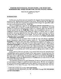
(i) for a ∈ [2], γa belongs to scan la and the input head in γa is scanning a symbol from vi0a ,φi (j 0 ) ; (ii) the a transition out of γ1 is a push transition (see Section 2); (iii) the transition out of γ2 is a pop transition; (iv) the stack height is the same in γ1 and in the configuration following γ2 ; and (v) the stack height is strictly higher in between them. Let BAD(M 0 , v 0 ) ⊆ [m] denote the set of instances that are corrupted in v 0 on M 0 . Intuitively, according to this definition, instance j is corrupted in input v(j, x, y) on Stack Machine M if M ever pushes a symbol on the stack in a transition that is to be simulated by player i1 , and later pops that same symbol in a transition that is to be simulated by another player i2 6= i1 . We claim that indeed, when j is not corrupted in v(j, x, y) on M , the protocol P can efficiently simulate M on v(j, x, y). Lemma 19. Let M 0 be a deterministic (r, s)-Stack Machine for f ∨,Φ . Let j ∈ [m] and let y ∈ (X p )m−1 . There exists a deterministic communication protocol P 0 = P 0 (M 0 , j, y) such that, on input x ∈ X p : (i) if j ∈ BAD(M 0 , v(j, x, y)), then P 0 outputs “fail”; (ii) otherwise, P 0 outputs M 0 (v(j, x, y)); and (iii) the cost of P 0 is O(p2 · (r(mnp))2 · s(mnp)). We defer the proof of this lemma to Appendix A.4. This lemma is the main part of the reduction. It is not hard to see how it is possible to efficiently detect whether j is corrupted in v. Assuming that j is not corrupted it is possible to efficiently simulate the Stack Machine; i.e. without communicating the entire stack content. Let us give an example so as to develop some intuition. Although the machine computation described in this example is among the simpler cases when it comes to efficient simulation by the players, this example does illustrate some of the main issues. Example for a special case of the efficient simulation. Consider the case of two players. Both players know the 0-inputs. We refer to the part of the 0-inputs as public input zone. If a stack symbol was pushed to the stack during the simulation of M 0 when the head was over a public zone then this stack symbol (for the corresponding time step and stack height) is a public stack symbol. This way we define the concept of public stack zone. Similarly, we define the private zones for Player-i. The symbols in the stack, have value (i.e. the actual symbol) and in addition we label them according to which zone the input head was when they were pushed in the stack. This distinction is necessary, because during the simulation, for a particular stack height a player may know the label of the input-zone associated with the stack symbol, but not the actual symbol. Consider the situation depicted on Figure 1 and suppose that the simulation has reached time t1 . On the right we depict the stack content which was created by M by computing on the input and by possibly making a few scans over the tape between time 0 and t1 . Furthermore, assume the invariant that up to time t1 each player knows: (i) the position (stack height) of every public and private stack-symbol, (ii) the symbol for each public stack symbol, (iii) Player-i knows her private stack symbols and (iv) the top stack symbol of the private stack zone which belongs to the other player. Player-1 will carry the simulation at this point since the input head enters her private zone. She can do the simulation up to time t2 where the head exits her private zone. As the simulation proceeds she pushes to the stack her private stack symbols and when she pops stack symbols these are either private to her or public. At time t2 it is not a good idea to send to Player-2 the stack height and the input-head position. The reason is that later on and as long as the head is over the public zone, the popped stack symbols enter at time t3 the private zone of Player-1 (and Player-2 does not know these stack symbols). Thus, Player-1 continues to simulate after t2 and up to the lowest level l4 of the stack with the input head over the public zone. At this point and since she knows this is the lowest level, she sends to Player-2 the stack height, the top stack symbol, and the position of the input head. Since this is the lowest stack height and the input head is over the publicly known zone both Players can independently reconstruct the public stack zone from time t4 all the way to time t5 , where Player-2 takes 19

Stack height

Stack content at t1

l1

l1

Public zone l3 l4

Player 1 zone .

t1

t2 t3

Input tape P1

t4

public (0-inputs)

t5

l3 l4

Stack content at t4 Player 1 zone

l4

.

.

.

.

.

time step

P2

Figure 1: On the upper part we depict how the stack height changes as a function of the simulation step of M 0 on the given input. On the right side of this upper part we depict the stack content at two different times. On the lower part we depict the input and which part of the input is known only to player 1, only to player 2 and which is known to both (public). over the simulation. This completes the description of the example. We would like to make sure that in protocol P , the probability that instance j is corrupted on v(j, x, y) is small. By construction, of the m inputs to f embedded in v(j, x, y), m − 1 of them are always 0-inputs. If, on the one hand, f (x) = 1, then instance j will be, intuitively, probabilistically distinguishable, so it is plausible that M dedicates the use of its stack to solving this instance, causing j to be corrupted in v(j, x, y). However, note that the protocol P 0 from Lemma 19 can detect that j is corrupted in v(j, x, y). So, in this case, the protocol P will simply output 1. If, on the other hand, f (x) = 0, then v(j, x, y) consists of m 0inputs to f . In the following Lemma (proof deferred in Appendix A.4), we use the property of the sequence of permutations Φ to give an upper bound on the number of instances that are corrupted in a fixed input v 0 . Lemma 20. Let M 0 be a deterministic (r, s)-Stack Machine for f ∨,Φ and let v 0 ∈ (X m )p . Then, we have √ |BAD(M 0 , v 0 )| ≤ O(p · r(mnp) · log(r(mnp)) · m). In the case f (x) = 0, if we were to show that the choice of j is statistically independent from v(j, x, y), the Lemma above would give us a bound for the probability that j is corrupted in v(j, x, y). A subtle point is that we cannot immediately prove this for every 0-input x. We overcome this by proving the statement distributionally, when x and the 0-inputs in y come from the same distribution. 8 To implement this intuition, we use Yao’s min-max principle that connects the randomized communication complexity of a function with its distributional complexity. 8

As explained in [BHN08], another way would be to observe that for the special case of f = P S ET I NT, any 0-input can be transformed into any other 0-input by a column permutation, and then modifying the protocol P to apply such a random permutation to x itself.

20

Proof of Theorem 13 (for the case when f = P S ET I NTp,n ). For every q, let Mq denote the deterministic (r, s)-Stack Machine obtained by running M with random string ρ. Let D be any distribution on the space X p of inputs to f . Below, we give a randomized protocol PD for f with cost and error as described in Theorem 13, but with error computed over the choice of the input x from D and of the random coins ρ. By standard arguments, we can fix ρ to obtain a deterministic protocol with the same error, but only over the choice of x from D. Since such a protocol exists for every distribution D, by Yao’s min-max principle (e.g., Theorem 3.20 in [KN97]), the conclusion of Theorem 13 follows. If D has support only on 0-inputs or only on 1-inputs, PD is trivial. Otherwise, let D0 = D conditioned on f (x) = 0. Consider the following protocol PD : On input x ∈ X p , where player i gets xi ∈ X, and shared random string ρ: Publicly draw j uniformly from [m] publicly draw y = (y 1 , . . . , y m−1 ) from D0m−1 publicly draw q uniformly Run P 0 = P 0 (Mq , j, y) (from Lemma 19) on input x, simulating Mq (v(x, j, y)) If P 0 outputs “fail”, then PD outputs 1. Else, PD outputs the same value as P 0 The cost of PD is equal to the cost of P 0 which is O(p2 (r(mnp))2 s(mnp)). To argue about the error in PD , define the following events: A = A(x, ρ): PD is correct on input x with coins ρ B = B(q, v): M is correct on input v with coins q and C = C(j, q, v): j ∈ / BAD(Mq , v). By Lemma 19, the simulation in P 0 fails if and only if C. Let α = Prx [f (x) = 0]. We write Pr[A] = α · Pr[A|f (x) = 0] + (1 − α) · Pr[A|f (x) = 1]. For the right term, consider the conditioning f (x) = 1. Then, PD is correct if either the simulation in P 0 fails (and PD correctly outputs 1), or the simulation in P 0 does not fail and M is correct, thus, C ∨ (C ∧ B) ⇒ A, in particular B ⇒ A, so Pr[A|f (x) = 1] ≥ Pr[B|f (x) = 1]. The event f (x) = 1 is independent of the choice of q, and by the correctness condition of M , ∀v, PrQ [B(Q, v)] ≥ (1 − δ). Hence, Pr[B|f (x) = 1] = Pr[B] ≥ (1 − δ). For the left term, consider the conditioning f (x) = 0. Then, PD is correct whenever the simulation in P 0 works and M is correct, thus B ∧ C ⇒ A, and Pr[A|f (x) = 0] ≥ Pr[B|f (x) = 0] Pr[C|B, f (x) = 0]. As before, Pr[B|f (x) = 0] ≥ (1 − δ). Next, j is clearly statistically independent of x and q. Furthermore, under the conditioning f (x) = 0, we claim that j is statistically independent from v. To see this, notice how the distribution obtained on pairs (j, v) in PD is the same as independently choosing m 0-inputs from D0 and combining them in v, and choosing j uniformly from [m]. Thus, in the expression Pr[C(j, q, v)|B(q, v), f (x) = 0], the conditioning depends on (x, v, q), C itself depends on j, and j is statistically independent from (x, v, q). By Lemma 20, ∀(q, v), PrJ [C(J, q, v)] ≥ (1 − d). Then, Pr[C|B, f (x) = 0] = Pr[C] ≥ (1 − d). Putting everything together gives the claimed error bound, Pr[A] ≥ 1 − (δ + d(1 − δ)). Remark 21. Theorem 13 states that if g = IPF2,n and M is a Stack Machine for g ⊕,Φ , we can build a similar protocol P for g. One can check that Definitions 17, 18, Lemmas 19 and 20 do not depend on either the “base” function f , or on the “combining” function ∨. Furthermore, one can check that even the proof for the case f = P S ET I NTp,n goes though if we replace f by g, and f ∨,Φ by g ⊕,Φ . Note that if we were to write 21

the proof for the case of g and g ⊕,Φ , we need not bother defining distribution D0 : the players in PD could simply draw y from Dm−1 (rather than D0m−1 ), because they could still compute g(x) from g ⊕,Φ (v(j, x, y)) by adding to the latter the outputs of the m − 1 inputs in y.

A.3

Proof of Corollaries 14 and 15

To prove Corollary 14, we need the following result. This reduction originates, in a non-permuted form, from [AMS99]. [BHN08] point out that the reduction still works for permuted instances of P S ET I NT. However, while [BHN08] make use of an additional external tape to make it work, we do not have that luxury when dealing with Stack Machines. We explain how to get the reduction to work with no additional tapes. Intuitively, the idea is that during the simulation we only need to look at a limited portion of the tape. We also slightly improve the dependency between parameters over [BHN08]. Theorem 22. Let  ≥ 0. Let M = mnp, with p ≥ (mn)Ω(1) . 1. Let k > 1 and p > (2(2 + )mn)1/k . Assume that, for large N , there exists a nonuniform (r, s)Stack Machine AN that, given a sequence a of N Θ(1) elements from [N Θ(1) ], outputs a (1 + )approximation of Fk (a). Then, for large M , there exists a nonuniform (r+2, s+O(log M ))-Stack Machine BM such that, when given an input v ∈ {0, 1}M , BM outputs f ∨,Φ (v), where f = P S ET I NTp,n . Moreover, if AN is randomized with error at most δ < 1/2, then so is BM . 2. The same holds when k < 1 and p > 2(2 + )mn/(1 + )2 . Proof of Theorem 22. First, consider the case k > 1. Let v ∈ {0, 1}mnp be an input to f ∨,Φ (v). To begin with, BM uses its first two reversals to count the number of 1s in v, storing this value as C on Θ(log M ) bits. If C < p, BM outputs 0, as none of the m instances of P S ET I NTp,n inside f ∨,Φ can contain an all-1 column. Similarly, if C > mn, BM outputs 1. To see this is correct, notice that by the promise, one 0-instance of P S ET I NTp,n contains at most n 1s, one in each column. Thus, m 0-instances of P S ET I NTp,n contain at most mn 1s. Henceforth, assume p ≤ C ≤ mn. Let N = C log(mn). Note that N ≤ mn log mn ≤ mnp = M since p = (mn)Ω(1) . Also, N ≥ p log mn ≥ M Ω(1) , so AN exists for large M . The machine BM simulates the machine AN on the following N -bit input stream a = a(v): for every (i, j, k) ∈ [p] × [m] × [n] such that vi,j,k = 1 (recall the notation from Definition 11), the stream a contains a value (φ−1 i (j) − 1)n + k ∈ [mn]. It is not hard to check the following property of this construction: If f ∨,Φ (v) = 0, the values in the stream a are distinct; and if f ∨,Φ (v) = 1, the stream a contains p occurrences of some value, and the rest are distinct. Suppose that BM can somehow simulate AN on input a. So, AN outputs a value y which is an (1 + )approximation of Fk (a). Note that: If f ∨,Φ (v) = 0, then Fk (a) = C, so y ≤ (1 + )C; and if f ∨,Φ (v) = 1, then Fk (a) = C − p + pk , so y ≥ (C + pk − p)/(1 + ). When p is larger than a constant, p < pk /2. Furthermore, by the assumption in the Theorem, pk > 2(2 + )mn ≥ 2(2 + )C. Rewriting, we obtain (C + pk − p) > (1 + )2 C, meaning that the ranges of y for f ∨,Φ (v) = 0 and f ∨,Φ (v) = 1 are disjoint. At this point, BM outputs 1 if y > (1 + )C. However, note that BM cannot simply write down a on a tape, so instead, BM will decode small portions of the stream containing a when they are needed. More precisely, BM holds in its memory: (i) a triple 22

(i, j, k) ∈ [p] × [m] × [n] on Θ(log M ) bits, initialized to (1, 1, 1), and always containing the player number, the instance number and the bit position of the location where the input head is scanning v; (ii) a buffer D of log mn = Θ(log M ) bits containing one element of a; (iii) the space s(N ) of the Stack Machine AN ; and (iv) extra O(1) bits. In total, BM uses space s(N ) + Θ(log M ) ≤ s(M ) + Θ(log M ). Before starting the simulation of AN , BM scans its input until it finds the first 1. It then writes in the buffer D the value (φ−1 i (j) − 1)n + k. >From now on, BM simulates AN , using its stack as the stack of AN , the reserved s(N )-bits as the memory of AN , and using D as the input tape for AN . Whenever AN attempts to move its head left/right of the buffer D, BM clears the buffer, moves its own input head left/right until it finds the first 1, refills D with the value (φi−1 (j) − 1)n + k, and resumes the simulation. It is easy to see that during this simulation, BM performs at most as many reversals as AN . Finally, if AN is randomized with error δ < 1/2, so is BM . For the case k < 1, the simulation is the same, but now for correctness we need C − (p − pk ) < C/(1 + )2 . This follows by taking p greater than a constant, so that pk < p/2, and using the new condition p > (2(2 + )mn/(1 + )2 ) ≥ 2(1 − 1/(1 + )2 )C. Proof of Corollary 14. Let β = (k − 5)/(9k + 9) > 0. Assume r = O(N β ) and s = O(N β ). We will derive a contradiction. Let α = (5k − 7)/(4k + 7), and let m = nα . Let p = (3(2 + )mn)1/k = O(1) · n(1+α)(1+1/k) (if  = 0, set p = 2). Let f = P S ET I NTp,n . Let r0 (M ) = r(M ) + 2 and let s0 (M ) = s(M ) + O(log(M )). By Theorem 22, there exists an (r0 , s0 )-SM BM for f ∨,Φ with error δ < 1/4. By Theorem 13, there exists a protocol for P S ET I NTp,n with cost O(p2 (r(mnp))2 s(mnp)) and error at most δ + d(1 − δ) where √ d = O(p(r(mnp))2 / m). Note that both r(mnp) and s(mnp) are O(n(1+α)(1+1/k)β ). One can check that, with the settings above, d = o(1), so for large n, the error of BM is at most, say 1/3. Then, by [CKS03], the cost of the protocol should be Ω(n/(p log p)). However, one can also check that, with the settings above, p2 (r(mnp))2 s(mnp) = o(n/(p log p)). This is a contradiction. Proof of Corollary 15. Similarly to the proof of Corollary 14, we use Theorem 13 to obtain an efficient protocol for IPF2,n , which requires Ω(n) communication.

A.4

Full proofs - omitted from the proof of Theorem 13

Proof of Lemma 19. Let x ∈ X p be an input to P 0 . The players share M 0 , j and y. The goal of P 0 is to simulate M 0 on input v = v(j, x, y). We say that an input symbol from v is private to player i if it belongs to vi,φi (j) , which is where xi , the input to player i, is embedded in v. Input symbols that are not private to any player are public. Private input symbols are never communicated in P 0 . Let Γ be the sequence of configurations of M 0 on input v. Consider γ ∈ Γ and look at the contents of the stack in γ. For every symbol ξ appearing on the stack, we say that stack symbol ξ is private to player i if during the transition when ξ was pushed on the stack, the input head was scanning an input symbol private to player i. (The same symbol may appear many times on the stack, so we should formally talk about a private stack level, rather than symbol, but we believe this degree of formalization negatively affects the intuition.) A stack symbol that is not private to any player is public. We say that player i sees a hollow view of the stack in configuration γ if player i knows: (i) the stack height in γ; (ii) for every symbol on the stack, whether it is public or the player to which it is private (that is, without knowing the symbol itself); (iii) all stack symbols that are public or private to player i; and (iv) for every i0 6= i, the top stack symbol in any contiguous zone of symbols private to player i0 . Note that the hollow views of different players of the same stack differ. We say that the players see a hollow view of

23

configuration γ if every player knows the state in γ, the input head position in γ, and sees a hollow view of the stack in γ. We say that configuration γ is input-private to player i if the input head is scanning an input symbol that is private to player i. We say that configuration γ is stack-private to player i if the transition out of γ is a pop transition and the top stack symbol in γ is private to player i. Intuitively, player i will be responsible for simulating the transitions out of configurations input- or stack-private to it. Note that there exists a configuration that is input-private and stack-private to two different players if and only if j ∈ BAD(M 0 , v). A configuration that is neither input-private nor stack-private is public. In the protocol P 0 , the players will simulate Γ transition by transition, always using hollow views of the configurations along the way. It is not hard to see that: (1) if a player sees a hollow view of the stack in a public configuration γ, then that player can compute a hollow view of the stack in configuration next(γ); (2) as long as j ∈ / BAD(M 0 , v), if player i sees a hollow view of the stack in a configuration γ which is input- or stack-private to player i, then player i can compute a hollow view of the stack in next(γ); and (3) if player i sees a hollow view of the stack in a configuration γ that is input-private to player i, it can detect whether γ is stack-private to another player i0 6= i. We now describe the protocol P 0 inductively. Clearly, all players see a hollow view of the initial configuration, because there is nothing on the stack. Inductively, assume all players see a hollow view of configuration γ. We consider three cases. Case 1: γ is public. By fact (1) above, each player can privately compute a hollow view of the stack in next(γ), so all players now see a hollow view of next(γ). Case 2: γ is input-private to player i. This means the input head is scanning vi,φi (j) in γ. All players recognize this because they know the input head position, so they give control of the simulation to player i. Let γ 0 be the first configuration following γ in Γ that is no longer input-private to player i. By applying facts (2) and (3) inductively, player i either detects that v ∈ BAD(M 0 , v) (in which case the simulation is aborted and protocol P 0 outputs “fail”), or it can compute hollow views of the stack in every configuration γ 00 between, and including, γ and γ 0 . Player i recognizes γ 0 is no longer input-private because it knows the input head position in γ 0 . At this point, player i communicates: (a) the state in γ 0 ; (b) the input head position in γ 0 ; (c) the stack height in γ 0 ; (d) the top stack symbol in γ 0 ; and (e) the lowest stack height L in any configuration γ 00 between γ and γ 0 , and the top stack symbol in γ 00 . We claim the information communicated is enough for a player i0 6= i to compute a hollow view of the stack in configuration γ 0 . Specifically, player i0 takes the hollow view of the stack from configuration γ, truncates it at height L, and fills it to the height in γ 0 with symbols private to player i. To compute part (iv) of the hollow view, player i0 obtains the top stack symbol in γ 0 from (d), and the stack symbol at level L from (e). Hence, after this communication, all players see a hollow view of configuration γ 0 . Case 3: γ is stack-private to player i (and not input-private). That is, the input head is scanning a public symbol, the transition out of γ is a pop transition, and the top stack symbol in γ is private to player i. All players recognize this situation, because they know whether the top stack symbol is private to player i, so they give control of the simulation to player i. Let γ 0 be the first configuration following γ in Γ that is either input-private (to any player) or stack-private to some player i0 6= i. By facts (1) and (2), player i can compute hollow views of the stack for every configuration γ 00 between, and including, γ and γ 0 . In order to best explain what player i communicates in case 3, we need to step back for a second and look at what we are trying to do: we are trying to design an efficient protocol P 0 , so we want to have as little communication as possible. Going backward from γ, let γa be the last configuration which is not inputprivate. Going forward from γ, let γb be the first configuration which is input-private. Let T denote the number of contiguous parts of input-private configurations before γa in Γ. During each reversal there are at

24

most p such parts, one corresponding to every player, and there are at most r reversals, so T ≤ pr. Looking at the stack in γa , observe that if we group together contiguous zones of stack symbols private to the same player, the number of such contiguous zones is at most T , the number of contiguous parts of input-private configurations before γa . Possibly all of these stack symbols are popped between γa and γb , but in order to keep the cost of the protocol low, we will devise a way in which communication occurs in P 0 at most T times, once for every zone of contiguous stack symbols private to some player. The discussion above suggest that in case 3 it would be a bad idea for player i to fall back to public simulation the moment it encounters a public configuration between γ and γ 0 : possibly that public configuration is closely followed by another stack-private configuration of player i, such that both the latter and γ correspond to the same contiguous zone of stack symbols in γa , which would invalidate the communication bound above. Another idea is to let player i perform the simulation all the way to γ 0 . This also turns out to be a bad idea, because, in general, stack symbols might have been pushed on the stack between γ and γ 0 , and those should not be private to any player, as the input head is in a public zone. Then, player i would have to actually communicate those symbols in order to give the other players a proper hollow view of γ 0 . Instead, we let γ ∗ be a configuration between, and including, next(γ) and γ 0 , where the stack height is the lowest possible (if there are several, any will do). Then, player i simulates only until γ ∗ , and it communicates items (a)—(d) as before, skipping (e). Again, we claim the information communicated is enough for a player i0 6= i to compute a hollow view of the stack in γ ∗ . This is simpler to see than in case 2 before, because, by choice of γ ∗ , it is enough for player i0 to truncate its hollow view of the stack in configuration γ to obtain a hollow view of the stack in γ ∗ . This completes the description of the protocol. If j ∈ / BAD(M 0 , v), one of the players gets to the final configuration and announces the output of the function. If j ∈ BAD(M 0 , v), one of the players detects this and outputs “fail”. To obtain the stated communication bound, we first observe that every communication takes O(s) bits. Because there are at most pr contiguous zones of input-private configurations, the communication generated by case 2 is at most O(prs) bits. Finally, by the discussion in case 3, at most pr communications occur during each contiguous zone of non-input-private configurations. There are pr − 1 such zones, to a total of O(p2 r2 s) bits. Proof of Lemma 20. We say that instance j ∈ BAD(M 0 , v 0 ) is corrupted by the tuple (l1 , l2 , i1 , i2 ) if the latter is the lexicographically smallest such tuple satisfying the conditions in Definition 18 for instance j. First, we consider the question of how many instances can be corrupted by one 4-tuple. Second, we argue that not all 4-tuples can simultaneously corrupt instances. Let J ⊆ [m] be k distinct instances that are corrupted by the same 4-tuple (l1 , l2 , i1 , i2 ). Recalling −1 −1 Definition 11, rename the instances in J in such a way that φ−1 i1 (j1 ) < φi1 (j2 ) < · · · < φi1 (jk ). Assume 0 that both l1 and l2 are odd. Then, the head of M scans vi1 during reversal l1 from left to right, So M 0 first visits vi1 ,φ−1 (j1 ) , then vi1 ,φ−1 (j2 ) , and so on, up to vi1 ,φ−1 (jk ) . For a ∈ [k], let γa,1 , γa,2 be the configurations i1

i1

i1

mentioned in Definition 18. By this definition, the stack level cannot drop between γa,1 and γa,2 , so then we must have γ1,1 ≺ γ2,1 ≺ · · · ≺ γk,1 ≺ γk,2 ≺ · · · ≺ γ2,2 ≺ γ1,2 . Since we assumed l2 is also odd, the head −1 −1 is also moving left to right in reversal l2 , so we obtain that φ−1 i2 (jk ) < · · · < φi2 (j2 ) < φi2 (j1 ). Then, −1 −1 −1 φ−1 φ−1 i2 ◦ φi1 (φi1 (j1 ) 0, C100 is followed by a pop transition, and C10 = next(C100 , x), where x is the top stack symbol in C1 . Lemma 25. The relation ≺ contains no cycles. Proof of Lemma 25. Assume a cycle exists. Let C1 , . . . , Cm be a sequence of surface configurations such that: C1 = Cm , and for every 1 ≤ i < m, Ci ≺ Ci+1 . Observe that whenever Ci ≺ Ci+1 , we have h(Ci ) ≤ h(Ci+1 ). Hence, h(C1 ) = h(Cm ) = h(Ci ) for all i ∈ [m], and so none of the Ci for i < m is followed by a toss transition. Furthermore, if Ci is followed by a pop transition, we cannot have Ci ≺ Ci+1 because such configurations create no dependencies. Hence, every one of the configurations in the sequence C1 , . . . , Cm is followed by either a move or a push transition. 0 But then, there is a path from a full configuration C1 to a full configuration C1 with the same surface C1 = Cm , with the stack level never dropping below that in C1 . Since this path only depends on the surface 0 C1 of C1 , and since C1 has the same surface, this path is infinite. We assumed C1 is reachable from the initial configuration of M , hence M does not halt along this path, a contradiction. To fill in the values in α(·, ·), we proceed as follows. 1. for all surface configs C, seen[C] ← false 2. find any surface config C1 such that seen[C10 ] for all C10 with C1 ≺ C10 3. for all surface configs C2 4. compute α(C1 , C2 ) using the formulas in Lemma 24 5. endfor 6. seen[C1 ] ← true 7. repeat step 2 as long there are unseen surface configurations 28

The test in step 2 can easily be implemented in the obvious way suggested by the definition of ≺. In the “most complex” case (iii-b), one can simply try out all possibilities for C100 , since there are only polynomially many of them. By Lemma 25, this algorithm does not get stuck at step 2. As an invariant, when line 6 is executed, all non-zero entries in the row α(C1 , ·) have been computed. Since there are polynomially many surface configs, the algorithm runs in polynomial time. 10

C

Variants of the model and omitted structural results

C.1 RPdL[poly] = RPdLE [poly] Lemma 26. RPdL[r(N )] ⊆ RPdLE [r(N )] ⊆ RPdL[O(r(N ))], where r(N ) = N O(1) . Proof of Lemma 26. The first inclusion is trivial. The second is also easy. Let L ∈ RPdL[r(N )], and let M be a SM such that for every x 6∈ L, M (x) rejects with probability 1 and for every x ∈ L, M (x) accepts with probability 12 . Moreover, the expected number of reversals on every input x is r(N ), |x| = N . Construct M 0 which on input x computes as follows. 1. Simulate M (x) for at most 4r(N ) reversals; count the reversals on the worktape. 2. If more than 4r(N ) reversals are needed then reject. 3. else do what M (x) does. Fix an input x. If x 6∈ L then M 0 outputs the correct answer with probability 1. Suppose that x ∈ L and let R be the random variable that corresponds to the number of reversals. By Markov’s inequality we have that Pr[R ≥ 4r(N )] ≤ 1/4, where r(N ) = E[R] by definition. First, using Markov’s inequality we show that Pr[M (x) rejects|R ≤ 4r(N )] ≤ 32 . The details of the calculations are given below. Then, by a different application of Markov’s inequality, together with the definition of 1 RPdLE [r(N )] we obtain that Pr[M 0 (x) rejects] ≤ 23 + 14 = 11 12 . This probability is amplified to ≤ 2 in the standard way, by considering a constant times larger random tape and use its bits for independent repetitions. This also increases the number of reversals by a constant factor. Here are the details of the calculations. First, we bound Pr[M (x) rejects|R ≤ 4r(N )] from above.

Pr[M (x) rejects] = Pr[R ≤ 4r(N )] Pr[M (x) rejects|R ≤ 4r(N )] + Pr[R > 4r(N )] Pr[M (x) rejects|R > 4r(N )] ≥ (1 − Pr[R > 4r(N )]) Pr[M (x) rejects|R ≤ 4r(N )] 3 ≥ Pr[M (x) rejects|R ≤ 4r(N )] 4 2 ⇒ Pr[M (x) rejects|R ≤ 4r(N )] ≤ 3 Then, 10

As a side note, observe that the algorithm might compute entries of the form α(C1 , C2 ) for unreachable C1 , because we cannot test whether C1 is reachable. These entries are useless (they are formally undefined), but also harmless, because well-defined entries never depend on undefined ones.

29

Pr[M 0 (x) rejects] = Pr[R ≤ 4r(N )] Pr[M 0 (x) rejects|R ≤ 4r(N )] + Pr[R > 4r(N )] Pr[M 0 (x) rejects|R > 4r(N )] = Pr[R ≤ 4r(N )] Pr[M (x) rejects|R ≤ 4r(N )] + Pr[R > 4r(N )] 2 1 11 ≤ Pr[M (x) rejects|R ≤ 4r(N )] + Pr[R > 4r(N )] ≤ + = 3 4 12

C.2

Non-deterministic variants

Proof of Theorem 3. NPdL[1] = P follows directly by the nontrivial Theorem 1 p.7 [Coo71]. By the NPcompleteness of 3-SAT under many-to-one logspace reductions, it suffices to decide 3-SAT in NPdL[2], since NPdL[2] is closed under logspace reductions. We describe a non-deterministic SM for 3-SAT. Let φ be the 3-CNF formula given in the input, with n variables x1 , . . . , xn and m clauses C1 , . . . , Cm . Let τ be a truth assignment identified by the string hτ (x1 ), . . . , τ (xn )i and let τ R denote the reversed string. Simultaneously, we: (i) check the truth assignment is a satisfying one; and (ii) check that the external tape is of the form hτ, τ R , . . . , τ, τ R , τ, τ R i. Associate | {z } m times

with the first clause C1 the first copy of the truth assignment τ , with C2 the second copy τ R , and so on up to Cm . To check (i) we do not use the stack, just the logspace worktape to verify that τ satisfies C1 , τ R satisfies C2 and so on. This verification can be done in one scan over the non-deterministic tape. To check (ii) we use the stack and the worktape as follows. Suppose that the external memory contains the strings w1 , . . . wn−1 , wn . In the first scan the machine uses the stack to verify that w1 = w2R , . . ., R , and w R R wn−3 = wn−2 n−1 = wn . When the head reverses it uses the stack to verify that wn−1 = wn−2 and so on. Intuitively, we first verify equality between mutually exclusive pairs and then we “link” them by verifying equality among the pairs. For Theorem 3 it is essential that the machine has a stack. In case of a regular log-space bounded TM the situation is very different. Recall that a log-space TM with a polynomially-long read-only non-deterministic tape characterizes NP. However, if we bound the number of reversals to be constant then we cannot go outside NL. We denote by L+ [r(N )] the class of sets decidable by logspace machines with external nondeterministic memory and r(N ) scans. Lemma 27. L+ [r(N )] ⊆ NSPACE(r(N ) log N ) Proof. We simulate a log-space r(N )-scan NTM M with a O(r(N ) log N ) space one-scan NTM M 0 . Fix an arbitrary branch of the non-deterministic computation; i.e. fix a choice of non-deterministic coins. We partition this branch of the computation according to the scan number. Associate each tape-scan 1, . . . , r(N ) with a part of this branch of the non-deterministic computation. here is how M 0 works. We begin by making r(N )-many non-deterministic guesses for the configurations for each part of the computation when the head is over the first symbol of the non-deterministic tape. We keep an additional copy (which we won’t modify during the simulation) for each of these r(N ) configurations corresponding to head-position over the first symbol. Storing each configuration takes space O(log N ). M 0 continues simulating M simultaneously (and step-by-step) for the r(N )-many parts of the computation. For the odd-numbered parts the 30

simulation moves forward in time, whereas for the even ones the simulation goes backwards in time (since the head has opposite direction). If the guesses are valid at some point the r(N ) parts of the computation are going to meet and form a valid branch of the non-deterministic computation. S + + Corollary 28. Let L+ [constant] := ∞ k=1 L [k]. Then, NL = L [constant]. Since with polynomially many reversals we go all the way to NP it is natural to ask what is the first time we capture P. Is it possible to capture P before we capture the whole NP? For instance, is it possible that P ⊆ L+ [N k ], for some constant k > 0? This is not true, unless P ⊆ NSPACE(N k log N ) ⊆ 0 DSPACE(N k ), for some constant k 0 .

D

Omitted proofs from Section 3 i

Proof of Theorem 4. P+RNCi ⊆ RPdL[2O(log N ) ] is the easy inclusion. Let L ∈ P+RNCi and M be the polytime transducer that on input x computes Cx . Construct a vSM M 0 as follows: use Cook’s algorithm [Coo71] to simulate M so as to obtain the k-th output bit from the description of Cx . Note that each bit is computed without accessing the random tape. M 0 evaluates Cx on the provided randomness in the usual way (e.g. [Ruz81]) by a depth first search. Note that if the description of the circuit were given through oracle i i access, the evaluation procedure would have taken time 2O(log N ) . Hence, M 0 makes at most 2O(log N ) reversals on the random tape and the accepting probability is the same as that of Cx . i To show RPdL[2O(log N ) ] ⊆ P+RNCi+1 we rely on the time-compression Lemma 7 and on [Ruz80, Ruz81]. In the version of the time-compression lemma for uniform machines, the advice can be computed i in polynomial time. Fix L ∈ RPdL[2O(log N ) ], and let M 0 be a vSM such that L(M 0 ) = L. We construct a polytime M that on input x outputs a circuit Cx with the same accepting probability as M 0 . There exists M 00 extending M 0 as follows: (1) M 00 has an extra input (read-only) tape which will contain the particular advice described in the proof of Lemma 7. (2) Furthermore, M 00 is a modification of M 0 as described in the proof of Lemma 7. Therefore, on input x given that the extra-tape contains this advice, M 00 computes identically to M 0 . Syntactically, M 00 is a SM with three read-only input tapes. When the 3rd tape i contains the appropriate advice, M 00 is a SM that works in space O(log N ) and in time 2O(log N ) N O(1) = i 2O(log N ) , i ≥ 1. We assert the existence of an equivalent ATM MATM that works in space O(log N ) and in time O(logi+1 N ). This is being done by observing that the corresponding equivalences carry through when the only difference is that both the SM and the ATM instead of one they have three input tapes. It is straightforward to verify that all equivalences between SMs and ATMs in the constructions of Theorem 5 part 3 [Ruz81] p.379 (i.e. Theorem 2 [Ruz80] pp. 227-231), and Corollary 3 (c,d,e) [Ruz81] pp. 379-380 are the same when the number of input tapes is a constant bigger than one. Hence, syntactically given the 3-input tape SM M 00 we have an ATM MATM with 3-input tapes that computes identically. The constant description of MATM it can be hardwired in a (polytime) TM M . Although MATM and M 00 accept the same inputs, we are only interested in the computations where their 3rd tape contains the advice of Lemma 7; in which case M 00 computes the same as M 0 . Intuitively, one can blur the distinction between space-time bounded ATMs and size-depth families of combinatorial circuits, and moreover we observe that given the description of the ATM we can construct efficiently the circuit for the corresponding input length. That is, the description of the polytime M should be evident through the observation that the construction in the proof of Theorem 3 [Ruz81] p.375 is computable in time 2O(S(N )) O(T (N ))N O(1) = N O(1) , where S(N ) = O(log N ) and T (N ) = O(logi+1 N ) is the space and the time of MATM . For completeness we briefly review this construction below.

31

1. On input x use (the modified) Cook’s algorithm to compute the advice of Lemma 7, which is a function of N = |x|. 2. M has hardwired the description of the ATM MATM and it computes the description of a circuit Cx . In this circuit, both the input x and the advice are hardwired using the constant 0/1 gates of the circuit. 3. The circuit gates are labelled with (α, t), where α is the configuration of the ATM, and t is the time where the output gates has label (αinitial , 0), where αinitial is the starting configuration. Configurations of type ∀, ∃ correspond to gates ∧, ∨, we connect gates (α, t), (β, t + 1) if α yields β. The only exceptions to this rule is when the time and the space becomes bigger than T (N ), S(N ) in which case we hardwire the gates to 0, and when we have configurations accessing the input in which case instead of a gate we have an input gate. Step (1) takes polynomial time. The construction of the circuit in Step 3, also takes polynomial time (2O(S(N )) O(T (N ))N O(1) ). Proof of Theorem 6. This is a straightforward argument, standard in derandomization. We show the stronger i i k containment RPdL[2O(log N ) ] ⊆ BPPdL[2O(log N ) ] ⊆ DTIME(2O(log N ) ). It directly follows that Theorem 4 holds also if we consider BPdL and P+BPNC, instead of RPdL and P+RNC. i Let L ∈ BPPdL[2O(log N ) ]. Then, there exists polytime transducer M that on input x outputs a circuit Cx of depth O(logi+1 N ), such that if x ∈ L then Prρ [Cx (ρ) = 1] ≥ 2/3, whereas if x 6∈ L then Prρ [Cx (ρ) = 1] ≤ 1/3, and the input to the circuit is of length N m , for a constant m > 0. We construct a ˆ that runs in time O(2logk N ). Here is the description of M ˆ : (1) Enumerate all strings deterministic TM M k k of length O(m log N ). (2) For each such string use the PRG to compute a string ρ of length N m . (3) Fix the random tape of M to be ρ and simulate M in polytime. (4) Output the majority of the outcome of the simulation. ˆ takes time 2O(logk N ) to enumerate all strings, for each such string it takes polynomial time to compute M ρ and then polynomial time to simulate M on (x, ρ). We claim that for infinitely many xi ’s: 11 (*) for input xi , at least a fraction 32 − 17 = 21 > 12 of the pseudorandom strings, M gives the correct answer, for sufficiently large input length N .

Note that the error probability in the definition of P+BPPdL can be amplified to any constant arbitrarily close to 1/2, and thus (*) suffices to conclude the theorem. Suppose (*) is not true. Then, we are going to use M to construct a (non-uniform) family of distinguishers DN , for infinitely many N ’s (where N takes values among the output length of the PRG). Let {xi } be an infinite family of inputs where (*) is false. Then, by definition Cxi is an appropriate distinguisher with 1 distinguishing probability strictly greater than 32 − 11 21 = 7 . Proof of Lemma 7. It suffices to show that the computation between two successive head-moves can be “compressed” to be polynomially long by the use of the non-uniform advice on the tape. This non-uniform advice extends the non-uniform advice already given to the machine. Fix two arbitrary successive headmoves. Partition the computation γ between these head-moves in two phases. Suppose that immediately after reading the input symbol the stack level is at l. In phase 1, γ reaches its lowest stack height lmin . Let γ1 be the computation subsequence of γ from the beginning until we reach the lowest stack level and just before we start going upwards (pushing symbols to the stack). Define γ2 to be the complement of γ1 wrt γ. Hence, in γ2 the computation reaches its final stack height llast . A simple counting argument shows 32

that for a halting SM, the stack height is polynomial, and therefore the stack height in γ1 gets decreased polynomially low (from l to lmin ) and in γ2 gets increased polynomially high (from lmin to llast ). We construct M 0 simulating M using the following non-uniform advice. The advice is a function from every surface configuration to the set of surface configuration together with two special symbols {↑, ↓}. For every surface configuration σ define exactly one of the three pairs: 1. If starting from σ we can return to the same stack level without ever going below the initial stacklevel (and without a head-move on the input) then consider the configuration after a maximally-long computation such that when M returns to the same stack-level the surface configuration is σ 0 . Then, the associated pair is (σ, σ 0 ). 2. If starting from σ we move at least one level upwards without ever returning to the initial stack-level (and without moving the head) then the pair is (σ, ↑). 3. Else, the pair is (σ, ↓). Obviously, this is a well-defined function and we say that a surface configuration σ is of type (1), (2) or (3) respectively. Between two successive head-moves M 0 simulates M by reading the advice tape and updating its surface configuration appropriately. In case of (1) it updates the worktape, the state and the top stack symbol. In case of (2) and (3) it simulates M for one step. We refer to a simulation step as the computation sequence of M 0 in which M 0 reads the non-uniform tape, compares it to the current surface configuration and updates the surface configuration appropriately. In what follows the reader is reminded that γ1 , γ2 is the computation of M which is simulated by the machine M 0 , and that M 0 is given the non-uniform advice. We say that a function from the integers is 2-monotonically increasing (decreasing) if it is strictly increasing (decreasing) for two successive integers; i.e. for the function h : Z+ → Z+ , h(n) ≤ h(n + 1) and h(n) < h(n + 2). Claim 29. In the simulation of γ1 the stack height in M 0 is 2-monotonically decreasing. Hence, this simulation takes at most 2(l − lmin ) simulation steps of M 0 . Proof. Consider two successive stack levels l1 > l2 := l1 − 1 in γ1 and consider the first time M 0 gets to l1 . The current surface configuration σ1 cannot be of type (2). Suppose that σ1 is of type (2). Since we are in γ1 we know that the stack level gets as low as lmin . If σ1 is of type (2) then we know that during γ1 the stack level will get back to l1 . Hence, σ1 should instead be of type (1). Hence, σ1 is either of type (1) or of type (3). If it is of type (3) there is nothing left to show. Suppose σ1 is of type (1). The fact that the next surface configuration in the simulation cannot be of the same type (1) follows by the maximality in the definition of type (1). Similarly, we show that in the simulation of γ2 the stack height in M 0 is 2-monotonically increasing. Proof of Lemma 8. In this proof all circuit classes are uniform. Suppose that the non-uniform advice can be ˆ be an SM that computes the advice string (i.e. the i-th bit of the output) computed in NC = SAC; i.e. let M in the proof of Lemma 7 in NC. We show that every polytime computable tally language L ⊆ {0}∗ can be computed in NC. By [All89] (Corollary 6.3 and Corollary 6.7) this implies that PSPACE = EXP. ˆ ) ∈ NC, by Theorem 1 we know that M works in time O(2logO(1) N ). Since, L(M Fix arbitrary L ⊆ {0}∗ , L ∈ P. Let M be a SM, such that L(M ) = L. O(1) N ), such that L(M 00 ) = L; i.e. L ∈ NC. We construct a SM M 00 , which works in time O(2log 33

Here is the description of M 00 . In a single tape-scan over 0N compute N and store it on the work-tape. Note that M 00 can simulate M on the given input, without moving its input head (also see Proposition 2.1 ˆ following this proof we can [All89]). Since the advice in the proof of Lemma 7 can be computed by M 0 construct a uniform M that decides L and it makes polynomial many calls to an oracle computing the advice ˆ in time O(2logO(1) N ). bit given its index. By assumption each oracle call can be computed by simulating M O(1) N ) = O(2logO(1) N ). Therefore, M 00 works in time O(N O(1) 2log

34