this, he used Hermite polynomials in terms of Gaussian random variables to represent Gaussian processes, which is referred to as homogeneous chaos.
Time-Dependent Polynomial Chaos Marc Gerritsma∗ , Peter Vos† and Jan-Bart van der Steen∗ ∗
Dept. Aerospace Engineering, TU Delft, Kluyverweg 1, 2629 HS Delft, The Netherlands Dept. Aeronautics, Imperial College, South Kensington Campus, London SW7 2AZ, UK
†
Abstract. Conventional generalized polynomial chaos is known to fail for long time integration, loosing its optimal convergence behaviour and developing unacceptable error levels. The reason for this loss of convergence is the assumption that the probability density function is constant in time. By allowing a probability density function to evolve in time the optimal properties of polynomial chaos are retrieved without resorting to high polynomial degrees. This time-dependent approach is applied to a system of coupled non-linear differential equations. These results are compared to the conventional generalized polynomial chaos solutions and Monte Carlo simulations. Keywords: Uncertainty, stochastic ODE, Kraichnan-Orszag problem polynomial chaos, long-term integration PACS: 05.00.00
GENERALIZED POLYNOMIAL CHAOS Generalized polynomial chaos (gPC) is employed to represent stochastic processes. Stochastic processes can be seen as processes involving some form of randomness. They can be represented by a stochastic mathematical model, often expressed in terms of stochastic differential equations. Stochastic mathematical models are based on a probability space (Ω, F , P) where Ω is the sample space, F ⊂ 2Ω its s -algebra of events, and P its probability measure. In addition considering some physical domain D ⊂ Rd × T (d = 1, 2, 3), which can be a combination of spatial and temporal dimensions, a stochastic process can be seen as a scalar- or vector-valued function u(x,t, w ) : D × Ω → Rb where x is an element of the physical space, t denotes the time and w is a point in the sample space Ω. Furthermore, because of the infinite-dimensional nature of the probability space, we discretize this space by characterizing it by a finite number of random variables {x j (w )}Nj=1 , N ∈ N. This can be seen as assigning a finite number of coordinates {x j }Nj=1 to the probability space reducing it to a finite dimensional space Λ ⊂ RN . Consequently, the stochastic process u becomes a mapping u(x,t, x ) : D × Λ → Rb . It is important to note that in this work, we assume that the occurring stochastic processes are already characterized by a known set of random variables. Wiener was the first to represent stochastic processes by orthogonal polynomial expansions [1]. To accomplish this, he used Hermite polynomials in terms of Gaussian random variables to represent Gaussian processes, which is referred to as homogeneous chaos. In this way, the stochastic process is represented in the form: ∞
u(x,t, x (w )) = ∑ ui (x,t)Hi (x (w ))
(1)
i=0
in which Hi are Hermite polynomials and x is a vector of Gaussian random variables with zero mean and unit variance. It is a spectral expansion in the random dimensions employing deterministic coefficients. According to the CameronMartin theorem [2], for a fixed value of x and t, this expansion converges to any L2 (Ω) functional in the L2 (Ω) sense. This implies that the application of polynomial chaos is restricted to those stochastic processes yielding Z
w ∈Ω
|u(x,t, w )|2 dP(w ) < ∞
(2)
As a result, polynomial chaos is restricted to second-order stochastic processes, i.e. processes with finite second-order moments. These are processes with finite variance, and this applies to most physical processes.
Although Wiener’s original polynomial chaos expansion converges to any second-order stochastic process, it is most suitable to represent Gaussian processes, due to the random variable’s Gaussian nature, yielding a fast convergence.
TABLE 1. The correspondence of the type of WienerAskey polynomial chaos and their underlying random variables Random variables x Wiener-Askey chaos {Φ j (x )} Gaussian Gamma Beta Uniform
Hermite-chaos Laguerre-chaos Jacobi-chaos Legendre-chaos
In order to deal with a broader range of stochastic processes, the Wiener-Hermite chaos has been generalized to the generalized polynomial chaos [3], also referred to as Wiener-Askey polynomial chaos. Analogously, gPC is a means of representing second-order stochastic processes through the expansion: ∞
u(x,t, x (w )) = ∑ ui (x,t)Φi (x (w ))
(3)
i=0
Here the random trial base {Φi (x (w ))} exists out of orthogonal polynomials from the Askey-scheme, of which the Hermite polynomials are a subset, in terms of a random vector x = {x j (w )}Nj=1 . The combination of random vector and polynomials is carefully selected based on the distribution of the random input. It seems that for certain random variables, their probability distribution function (PDF) uniquely corresponds to one of the weighting functions w(x ) in the orthogonality relation of the different orthogonal polynomials of the Askey-scheme. An overview of this correspondence is shown in Table 1. Choosing the corresponding combination leads to a proper gPC expansion. Since each of the polynomials of the Askey-scheme forms a complete basis in the Hilbert space determined by their corresponding support, it is expected, according to Xiu et al. [3], that each type of Wiener-Askey expansion converges to any L2 (Ω) functional in the L2 (Ω) sense in the corresponding Hilbert functional space as a generalized result of Cameron-Martin theorem. The polynomials of the gPC’s random trial base satisfy following orthogonality relation hΦi Φ j i = hΦ2i idi j
(4)
where di j is the Kronecker delta and h·, ·i denotes the ensemble average. The inner product in (4) is in the Hilbert space determined by the measure of the random variables h f (x )g(x )i =
Z
w ∈Ω
f (x )g(x )dP(w ) =
Z
f (x )g(x )w(x )d x
(5)
with w(x ) the corresponding weighting function and with integration in the last integral taken over the support of x .
LONG-TERM INTEGRATION It is known that the generalized polynomial chaos method looses its accuracy for long time integration. The reason for this breakdown is that in the unsteady case the probability density function changes in time and therefore new orthogonal polynomials need to be generated. The idea is therefore to perform a transformation at a certain time of the stochastic variables of the form P
∗ zi = xi (t ∗ , xi ) = ∑ x(i) p (t )Φ p (xi ) ,
(6)
p=0
where xi (t ∗ , xi ) is the solution of the random variable xi at time t ∗ . The orthogonal polynomials associated with the probability distribution of zi are generated by a modified Gramm-Schmidt orthogonalization. Note that in the new stochastic variable, zi , the function xi can be represented exactly as a linear function in zi , i.e. an expansion with P = 1 is exact. As time progresses, higher order modes in zi will appear in the solution. If these higher order modes become large, new random variables are created using the transformation rule (6). This method was originally developed by Vos, [4].
1
Mean(x1)
0.5
0
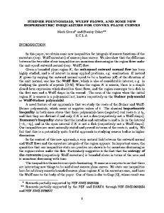
TDgPC P = 2 gPC P = 2 MC N = 131072
-0.5
0
10
20
30
40
t FIGURE 1. Mean of x1 vs. time for a = 0.99, b = 1 and g = 1: TDgPC solution (P = 2) compared to a gPC solution (P = 2) and a Monte Carlo analysis (N = 131072)
This approach is applied to the Kraichnan-Orszag problem which is known to lead to inaccurate solutions for certain initial conditions: dx1 = x2 x3 dt dx2 = x3 x1 dt dx3 = −2x1 x2 dt
(7a) (7b) (7c)
We solve this set of equations subject to the following initial conditions x1 (0) = a + 0.01x1 ,
x2 (0) = b + 0.01x2 ,
x3 (0) = g + 0.01x3
(8)
where a , b and g are constants and x1 , x2 and x3 are uniformly distributed random variables on the interval [−1, 1]. x1 , x2 and x3 are statistically independent. We take a = 0.99, b = 1.0 and g = 1.0. Following the TD-gPC approach, new random variables are generated for each of the three variables and therefore the probability distribution of each variable will differ. As a consequence, three polynomial sets need to be constructed to represent the uncertainty in xi . The joint probability distribution is not assumed to be statistically independent.
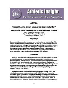
RESULTS Figures. 1 and 2 show the comparison of the TDgPC solution approach with results obtained with a gPC solution approach and a Monte Carlo analysis. The gPC method departs from the Monte-Carlo result at approximately t = 4. The TD-gPC method follows the Monte Carlo results quite well up to t = 40. A comparison of results for x2 or x3 would show similar characteristics. Note that these results were obtained with a relatively low polynomial degree of P = 2.
Var(x1)
0.6
0.4
0.2 TDgPC P = 2 gPC P = 2 MC N = 131072 0
0
10
20
30
40
t FIGURE 2. Variance of x1 vs. time for a = 0.99, b = 1 and g = 1: TDgPC solution (P = 2) compared to a gPC solution (P = 2) and a Monte Carlo analysis (N = 131072)
CONCLUSIONS A novel technique is presented to solve stochastic differential equations. The method adapts gPC in time. Due to this adaptation there is no need to go to very high polynomial order. The method works with the joint probability distribution and does not assume statistic independence. The method is much more accurate than gPC which only employs Legendre polynomials.
REFERENCES 1. 2. 3. 4.
N. Wiener, The Homogeneous Chaos, Amer. J. Math., 60, 897-936, (1938). R. Cameron and W. Martin, The orthogonal development of nonlinear functionals in series of Fourier-Hermite functionals, Ann.MAth., Vol. 48, Issue 2, 385-392, (1947). D. Xiu and G.E. Karniadakis, Wiener-Askey polynomial chaos for stochastic differential equations, SIAM J. Sci. Comput., Vol 24(2), 619-644, (2002) P.E.J. Vos and M.I. Gerritsma, Application of the least-squares spectral element method to polynomial chaos, in proceeding of ECCOMAS CFD 2006, 5-8 September 2006, Egmond aan Zee, The Netherlands


![[hal-00770006, v1] Identification of polynomial chaos](https://m.moam.info/img/260x300/hal-00770006-v1-identification-of-polynomial-chaos_5c3dd1ef097c47a6158b45a1.jpg)


