Pre-Computable Multi-Layer Neural Network Language Models Jacob Devlin Microsoft Research Redmond, WA, USA
[email protected]
Chris Quirk Microsoft Research Redmond, WA, USA
[email protected]
Abstract
[email protected]
One popular application of neural network models in NLP is using neural network language models (NNLMs) as an additional feature in an existing machine translation (MT) or automatic speech recognition (ASR) engines. NNLMs are particularly costly in this scenario, since decoding a single sentence typically requires tens of thousands or more n-gram lookups. Although we will focus on this particular scenario in this paper, it is important to note that the techniques presented generalize to any feed-forward embedding-based neural network model. One popular technique for improving the runtime speed of NNLMs involves training the network to be “approximately normalized,” so that the softmax normalizer does not have to be computed after training. Two algorithms have been proposed to achieve this: (1) noise-contrastive estimation (NCE) (Mnih and Teh, 2012; Vaswani et al., 2013) and (2) explicit self-normalization (Devlin et al., 2014), which is used in this paper. However, even with self-normalized networks, computing the output of an intermediate hidden layer still requires a costly matrix-vector multiplication. To mitigate this, Devlin et al. (2014) made the observation that for 1-layer NNLMs, the dot product between each embedding+position pair and the first hidden layer can be pre-computed after training is complete, which allows the matrixvector multiplication to be replaced by a handful of vector additions. Using these two techniques in combination improves the runtime speed of NNLMs by several orders of magnitude with no degradation to accuracy. To understand pre-computation, first assume that we are training a NNLM that uses 250dimensional word embeddings, a four word context window, and a 500-dimensional hidden layer. The weight matrix for the first hidden layer is thus 1000 × 500. For each word in the vocabulary and each of the four positions in the context vector, we
In the last several years, neural network models have significantly improved accuracy in a number of NLP tasks. However, one serious drawback that has impeded their adoption in production systems is the slow runtime speed of neural network models compared to alternate models, such as maximum entropy classifiers. In Devlin et al. (2014), the authors presented a simple technique for speeding up feed-forward embedding-based neural network models, where the dot product between each word embedding and part of the first hidden layer are pre-computed offline. However, this technique cannot be used for hidden layers beyond the first. In this paper, we explore a neural network architecture where the embedding layer feeds into multiple hidden layers that are placed “next to” one another so that each can be pre-computed independently. On a large scale language modeling task, this architecture achieves a 10x speedup at runtime and a significant reduction in perplexity when compared to a standard multilayer network.
1
Arul Menezes Microsoft Research Redmond, WA, USA
Introduction
Neural network models have become extremely popular in the last several years for a wide variety of NLP tasks, including language modeling (Schwenk, 2007), sentiment analysis (Socher et al., 2013), translation modeling (Devlin et al., 2014), and many others (Collobert et al., 2011). However, a serious drawback of neural network models is their slow speeds in training and test time (runtime) relative to alternative models such as maximum entropy (Berger et al., 1996) or backoff models (Kneser and Ney, 1995). 256
Proceedings of the 2015 Conference on Empirical Methods in Natural Language Processing, pages 256–260, c Lisbon, Portugal, 17-21 September 2015. 2015 Association for Computational Linguistics.
functions are explored rather than just the max function.
2 Lateral Network In a standard feed-forward embedding-based neural network, the input tokens are mapped into a continuous vector using an embedding table1 , and this embedding vector is fed into the first hidden layer. The output of each hidden layer is then fed into the next hidden layer. We refer to this as the stacked architecture. For a two layer network, we can represent the output of the final hidden layer as:
Figure 1: The “pre-computation trick.” The dot product between each word embedding and each section of the hidden layer can be computed offline.
H = φ(W2 φ(W 1 E(x))) where x is the input vector, E(x) is the output of the embedding layer, Wi is the weight matrix for layer i, and φ is the transfer function such as tanh. Generally, H is then multiplied by an output matrix and a softmax is performed to obtain the output probabilities. In the lateral network architecture, the embedding layer is fed into two or more “side-by-side” hidden layers, and the outputs of these hidden layers are combined using an element-wise function such as maximum or multiplication. This is represented as:
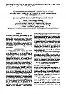
Figure 2: Network architectures. can pre-compute the dot product between the 250dimensional word embedding and the 250 × 500 section of the hidden layer. This results in four 500-dimensional vectors for each word that can be stored in a lookup table. At test time, we can simply sum four vectors to obtain the output of the first hidden layer. This is shown visually in Figure 1. Note that this is not an approximation, and the resulting output vector is identical to the original matrix-vector product. However, the major limitation of the “pre-computation trick” is that it only works with 1-hidden layer architectures, even though more accurate models can nearly always be obtained by training multi-layer networks. In this paper, we explore a network architecture where multiple hidden layers are placed “next to” one another instead of “on top of” one another, as is usually done. The output of these lateral layers are combined using an inexpensive elementwise function and fed into the output layer. Crucially, then, we can apply the pre-computation trick to each hidden layer independently, allowing for very powerful models that are orders of magnitude faster at runtime than a standard multi-layer network. Mathematically, this can be thought of as a generalization of maxout networks (Goodfellow et al., 2013), where different element-wise combination
H = C(φ(W 1 E(x)), φ(W 2 E(x))) Where C is a combination function that takes two or more k-dimensional vectors as inputs and produces as k-dimensional vector as output. If C(h1 , h2 ) = max(h1 , h2 ) then this is equivalent to a maxout network (Goodfellow et al., 2013). To generalize this, we explore three different combination functions: 2 Cmax (h1 , h2 ) = max(h1 , h2 ) Cmul (h1 , h2 ) = h1 ∗ (h2 + 1) Cadd (h1 , h2 ) = h1 + h2 The three-or-more hidden layer versions are constructed as expected.3 A visualization is given in Figure 2. Crucially, for the lateral architecture, each hidden layer can be pre-computed independently, allowing for very fast n-gram probability lookups at runtime. 1 The embeddings may or may not be trained jointly with the rest of the model. 2 Note that C is an element-wise function, so these represent the operation on a single dimension of the input vectors. 3 The + 1 in Cmul is used for all hidden layers after the first. This is used to prevent the value from being very close to 0.
257
3
Condition 5-gram KNLM 1-Layer (k=500) 1-Layer (k=1000) 2-Stacked (k=500) 2-Stacked (k=1000) 3-Stacked (k=1000) 2-Lateral Max (k=500) 2-Lateral Mul ... 2-Lateral Add 3-Lateral Max 3-Lateral Mul 3-Lateral Add
Language Modeling Results
In this section we report results on a large scale language modeling task. 3.1
Data
Our LM training corpus consists of 120M words from the New York Times portion of the English GigaWord data set. This was chosen instead of the commonly used 1M word Penn Tree Bank corpus in order to better represent real world LM training scenarios. We use all data from 2008 and 2009 as training, the first 100k words from June 2010 as validation, and the first 100k words from December 2010 as test. The data is segmented and tokenized using the Stanford Word Segmenter with default settings. 3.2
Table 1: Perplexity of 5-gram models on the New York Times test set. k is the size of the hidden layer(s).
Neural Network Training
Training was performed with an in-house toolkit using stochastic gradient descent. The vocabulary is limited to 16k words so that the output layer can be trained using a basic softmax with self-normalization. All experiments use 250dimensional word embeddings and a tanh activation function. The weights were initialized in the range [-0.05, 0.05], the batch size was 256, and the initial learning rate was 0.25. 3.3
PPL 91.1 77.9 77.7 76.3 76.2 74.8 73.8 72.7 73.7 73.1 71.1 72.3
3.4
Runtime Speed
The runtime speed of the various models is shown in Table 2. These are computed on a single core of a E5-2650 2.6 GHz CPU. Consistent with Devlin et al. (2014), we see that the baseline model achieves only 230 n-gram lookups per second (LPS) at test time, while the pre-computed, self-normalized 1-layer network achieves 600,000 LPS. Adding a second stacked layer slows this down to 24,000 LPS due to the 500 × 500 matrix-vector multiplication that must be performed. However, the lateral configuration achieves 305,000 LPS while obtaining a better perplexity than the stacked network. In comparison, the fastest backoff LM implementation, KenLM (Heafield, 2011), achieves 1-2 million lookups per second. In terms of memory usage, it is difficult to fairly compare backoff LMs and NNLMs because neural networks scale linearly with the vocabulary size, while backoff LMs scale linearly with the number of unique n-grams. In this case, the nonprecomputed neural network model is 25 MB, and the pre-computed 2-lateral network is 136 MB.4 The KenLM models are 1.1 GB for the Probing model and 317 MB for the Trie model. With a vocabulary of 50k, the 2-lateral network would be 425MB. In general, a pre-computed NNLM is comparable to or smaller than an equivalent backoff LM in terms of model size.
5-gram LM Perplexity
5-gram results are shown in Table 1. The 1-layer NNLM achieves a 13.2 perplexity improvement over the Kneser-Ney smoothed baseline (Kneser and Ney, 1995). Consistent with Schwenk et al. (2014), using additional hidden layers to the stacked (standard) network results in 2.0-3.0 perplexity improvements on top of the 1-layer model. The lateral architecture significantly outperforms any of the stacked networks, achieving a 6.5 perplexity reduction over the 1-layer model. The multiplicative combination function performs better than the additive and max functions by a small margin, which suggests that it better allows for modeling complex relationships between input words. Perhaps most surprisingly, the additive function performs as well as the max function, despite the fact that it provides no additional modeling power compared to a 1-layer network. However, it does allow the model to generalize better than a 1-layer network by explicitly tying together two or three hidden nodes from each node in the output layer.
4 The floats can be quantized to 2 bytes after training without loss of accuracy.
258
Condition KenLM Probing KenLM Trie 1-Layer (No PC, No SN) 1-Layer (No PC) 1-Layer 2-Stacked 2-Stacked (Batch=128) 2-Lateral Mul
Lookups Per Sec. 1,923,000 950,000 230 13,000 600,000 24,000 58,000 305,000
Condition Baseline +NNLM 1-Layer +NNLM 2-Stacked +NNLM 2-Lateral +NNJM 1-Layer +NNJM 2-Stacked +NNJM 2-Lateral
space, since they require a fully expanded target context. Second, the matrix-vector product between the previous hidden state and the hidden weight matrix cannot be pre-computed, which makes the models significantly slower than precomputable feed-forward networks.
4 High-Order LM Perplexity
Machine Translation Results
Although the lateral networks achieve a significant reduction in LM perplexity over the 1-layer network, it is not clear how much this will improved performance in a downstream task. To evaluate this, we trained two neural network models for use as additional features in a machine translation (MT) system. The first feature is a 5-gram NNLM, which used 1000 dimensions for the stacked network and 500 for the lateral network. The second feature is a neural network joint model (NNJM), which predicts each target word using 5-gram target context and 7-gram source context. For evaluation, we present both the model perplexity and the BLEU score when using the model as an additional MT feature. Results are presented on a large scale EnglishGerman speech translation task. The parallel training data consists of 600M words from a variety of sources, including OPUS (Tiedemann, 2012) and a large in-house web crawl. The baseline 4-gram Kneser-Ney smoothed LM is trained on 7B words of German data. The NNLM and NNTMs are trained only on the parallel data. Our MT decoder is a proprietary engine similar to Moses (Koehn et al., 2007). The tuning set consists of 4000 utterances from conversational and newswire data, and the test set consists of 1500 sentences of collected conversational data. Results are show in Table 4. We can see that perplexity improvements are similar to what is
We also report results on a 10-gram LM trained on the same data, to explore whether the lateral network can achieve an even higher relative gain when a large input context window is available. Results are shown in Table 3. Although there is a large absolute improvement over the 5-gram LM, the relative improvement between the 1-layer, 3stacked, and 3-lateral systems are similar to the 5-gram scenario. Condition 1-Layer (k=500) 3-Stacked (k=1000) 3-Lateral Mul (k=500) Gated Recurrent (k=1000)
Test PPL 138.3 136.2 132.3 6.33 6.25 6.13
Table 4: Results on English-German machine translation test set.
Table 2: Runtime speed of the 5-gram LM on a single CPU core. “PC” = pre-computation, “SN” = self-normalization, which are used in all but the first two experiments. The batch size is 1 except when specified. 500-dimensional hidden layers are used in all cases. “Float Ops.” is the approximate number of floating point operations per lookup. 3.5
Test BLEU 37.95 38.89 39.13 39.15 40.71 40.82 40.89
PPL 69.8 65.8 63.4 55.4
Table 3: Perplexity of 10-gram models on the New York Times test set. The Gated Recurrent model uses the full word history. As another point of comparison we report results with an gated recurrent network (Cho et al., 2014). As is consistent with the literature, the recurrent network significantly outperforms any of the feed-forward models (Sundermeyer et al., 2013). However, recurrent models have two major downsides. First, they cannot easily be integrated into existing MT/ASR engines without significantly altering the search algorithm and search 259
seen in the English NYT data, and that improvements in BLEU over a 1-layer model are small but consistent. There is not a significant difference in BLEU between the 2-Stacked and 2-Lateral configuration.
5
In Acoustics, Speech, and Signal Processing, 1995. ICASSP-95., 1995 International Conference on. Philipp Koehn, Hieu Hoang, Alexandra Birch, Chris Callison-Burch, Marcello Federico, Nicola Bertoldi, Brooke Cowan, Wade Shen, Christine Moran, Richard Zens, et al. 2007. Moses: Open source toolkit for statistical machine translation. In Proc. Assoc. for Computational Linguistics (ACL).
Conclusion
In this paper, we explored an alternate architecture for embedding-based neural network models which allows for a fully pre-computable network with multiple hidden layers. The resulting models achieve better perplexity than a standard multilayer network and is at least an order of magnitude faster at runtime. In future work, we can assess the impact of this model on a wider array of feed-forward embedding-based neural network models, such as the DSSM (Huang et al., 2013).
Andriy Mnih and Yee Whye Teh. 2012. A fast and simple algorithm for training neural probabilistic language models. In Proceedings of the International Conference on Machine Learning. Holger Schwenk, Fethi Bougares, and Loıc Barrault. 2014. Efficient training strategies for deep neural network language models. In NIPS Workshop on Deep Learning and Representation Learning. Holger Schwenk. 2007. Continuous space language models. Computer Speech & Language. Richard Socher, Alex Perelygin, Jean Y Wu, Jason Chuang, Christopher D Manning, Andrew Y Ng, and Christopher Potts. 2013. Recursive deep models for semantic compositionality over a sentiment treebank. In EMNLP.
References Adam L Berger, Vincent J Della Pietra, and Stephen A Della Pietra. 1996. A maximum entropy approach to natural language processing. Computational linguistics.
Martin Sundermeyer, Ilya Oparin, Jean-Luc Gauvain, Ben Freiberg, Ralf Schluter, and Hermann Ney. 2013. Comparison of feedforward and recurrent neural network language models. In Proc. Conf. Acoustics, Speech and Signal Process. (ICASSP).
Kyunghyun Cho, Bart van Merrienboer, C¸aglar G¨ulc¸ehre, Fethi Bougares, Holger Schwenk, and Yoshua Bengio. 2014. Learning phrase representations using RNN encoder-decoder for statistical machine translation. CoRR.
J¨org Tiedemann. 2012. Parallel data, tools and interfaces in opus. In LREC. Ashish Vaswani, Yinggong Zhao, Victoria Fossum, and David Chiang. 2013. Decoding with large-scale neural language models improves translation. In EMNLP.
Ronan Collobert, Jason Weston, L´eon Bottou, Michael Karlen, Koray Kavukcuoglu, and Pavel Kuksa. 2011. Natural language processing (almost) from scratch. The Journal of Machine Learning Research. Jacob Devlin, Rabih Zbib, Zhongqiang Huang, Thomas Lamar, Richard Schwartz, and John Makhoul. 2014. Fast and robust neural network joint models for statistical machine translation. In ACL. Ian J Goodfellow, David Warde-Farley, Mehdi Mirza, Aaron Courville, and Yoshua Bengio. 2013. Maxout networks. arXiv preprint arXiv:1302.4389. Kenneth Heafield. 2011. Kenlm: Faster and smaller language model queries. In Proceedings of the Sixth Workshop on Statistical Machine Translation. Po-Sen Huang, Xiaodong He, Jianfeng Gao, Li Deng, Alex Acero, and Larry Heck. 2013. Learning deep structured semantic models for web search using clickthrough data. In Proceedings of the 22nd ACM international conference on Conference on information & knowledge management. ACM. Reinhard Kneser and Hermann Ney. 1995. Improved backing-off for m-gram language modeling.
260