Nov 5, 2001 - GPS relative navigation for spacecraft autonomous ren- dezvous and ... Center (GSOC). ... pseudorange and carrier phase measurements via a serial ... In a near-circular orbit, the evolution of this rela- ..... It comprises a total of 28 healthy satellites (all PRNs except. 12, 16, 19, 32). ... obscuration angle.
Precise Spacecraft Relative Navigation Using Kinematic Inter-Spacecraft State Estimates T. Ebinuma† , O. Montenbruck‡ , and E. G. Lightsey† † The University of Texas at Austin, USA ‡ Deutsches Zentrum f¨ur Luft- und Raumfahrt (DLR), Germany
BIOGRAPHY
further reduction of residual errors left in the kinematic relative navigation solutions and for propagation across short GPS outages. The potential of a Hill’s equations model and a J2 propagator for this purpose are discussed.
Dr. Takuji Ebinuma is a postdoctoral fellow at Center for Space Research (CSR). His current activities focus on GPS relative navigation for spacecraft autonomous rendezvous and satellite formations. He received his Ph.D. in Aerospace Engineering from University of Texas at Austin. Dr. Oliver Montenbruck is head of the GPS Technology and Navigation Group at the German Space Operations Center (GSOC). His current field of work comprises the development of on-board navigation systems and spaceborne GPS applications. He has written various text books on computational astronomy and satellite orbits. He received his Ph.D. from University of Technology at Munich, Germany. Dr. E. Glenn Lightsey is an Assistant Professor in the Aerospace Engineering and Engineering Mechanics Department. He was formerly an Aerospace Engineer at NASA Goddard Space Flight Center and works on the design and testing of spaceborne GPS receivers. He received his Ph.D. in Aeronautics and Astronautics from Stanford University.
INTRODUCTION New mission concepts require precise relative navigation and control of multiple spacecraft formations to achieve desired science objectives. Example missions include synthetic aperture imaging and optical interferometry. In order to reduce overall mission cost, it is desirable to perform autonomous relative navigation of the formation using onboard sensors. The Global Positioning System (GPS) sensors can be applied advantageously to autonomous relative navigation with communication links among the satellites in the formation. To support this effort, a pair of prototype GPS relative navigation sensors has been developed based on the GPS Orion 12-channel L1 receivers. By exchanging raw pseudorange and carrier phase measurements via a serial data link between them, each receiver processes differential measurements internally and provides purely kinematic relative state estimates of the peer spacecraft without help of external navigation systems. The differential processing provides a high level of common error cancellation over baselines of typically less than 10 km and effectively eliminates the impact of broadcast ephemeris and ionospheric delay errors. Instead of performing integer ambiguity resolution, the GPS relative sensor utilizes carrier smoothed pseudorange measurements. The carrier smoothing process requires much less computational effort than the integer ambiguity resolution algorithms and is well suited for accommodation within the limited processor capacity of a GPS Orion receiver. By smoothing the differential pseudoranges with differential carrier phase measurements, a pronounced reduction of the relative position noise level is achieved. In view of the small relative velocity, time differences of the single-differenced carrier phase provide
ABSTRACT A prototype implementation of a spaceborne relative navigation sensor based on a pair of GPS Orion 12-channel L1 receivers is presented. It employs two individual receivers exchanging their raw measurements via a dedicated serial data link. Besides computing its own navigation solution, each receiver processes single difference measurements to obtain the relative state. The prototype receivers have been qualified with hardware-in-the-loop tests using a GPS signal simulator. They provide relative navigation solution accuracies of 0.5 m and 0.5 cm/s for position and velocity, respectively. While the purely kinematic relative navigation meets the accuracy requirements of many applications in the area of spacecraft rendezvous and formation flying, a highly simplified dynamic filter can be applied for ION GPS 2002, 24-27 September 2002, Portland, OR
2038
an excellent approximation of the instantaneous differential range-rate, which also allows a highly accurate determination of the inter-satellite velocity vector. For ease of use, the relative state is provided in a co-moving frame aligned with the radial, cross-track, and along-track directions. In a near-circular orbit, the evolution of this relative state vector can then approximately be described by the well-known Hill’s equations, which is useful for a rapid forecast in rendezvous-type proximity operations or for an optional dynamic filtering. For a qualification of these newly developed relative navigation sensors, intensive hardware-in-the-loop simulations were conducted using a closed-loop GPS test facility. The core component of the facility is a Spirent STR4760 GPS signal simulator capable of simultaneously simulating L1 signals for two vehicles on up to 16 channels each. Each receiver is connected to one of the RF outputs of the simulator via a coaxial cable. The Orion receiver has two serial data ports. One of them is used to send the raw measurements to an external device (e.g. onboard processor or monitoring and control PC) and the other is dedicated to the inter-spacecraft data link. For laboratory testing, the interspacecraft link ports of the two receivers are connected directly via a serial cable or a simple radio modem. The kinematic relative navigation performance was evaluated for a pair of formation flying satellites in a polar orbit with 10 km along track separation. The test results show that overall accuracies of 0.5 m relative positioning and 0.5 cm/s or less relative velocity are achievable. The purely kinematic relative navigation solutions are rapid and robust, but less accurate than the filter state estimates obtained in an earlier research activity [1] using an extended Kalman filter with a higher-dimensional dynamic model. However, this type of dynamic filter generally requires a dedicated navigation processor, which is not suitable for platforms with restricted onboard resources. On the other hand, in combination with the GPS relative navigation sensor, a simple linear Kalman filter using Hill’s equations or a J2 propagator can provide a reasonable filter state accuracy with notably reduced processor requirements. Compared to a rigorous dynamic filtering, the hardware and software requirements are considerably reduced at tolerable loss in overall precision. A minimal computational requirement for an external navigation processor can provide a compact relative navigation package that is highly optimized for small satellites, which are expected to be the platforms for distributed formation flying missions.
with a capacity of 256 kB. Typical code size of the software ranges from 160-200 kB. To support user specific software adaptations for the GPS Orion receiver, the GPS Architect development kit was made available by Mitel [3].
Fig. 1 GPS Orion Receivers For use on low Earth orbit satellites and other space applications, numerous software modifications and enhancements have been made to the original firmware of the Orion receiver [4]. These modifications include the fixes related to the implicit assumption of a low speed vehicle in the Doppler prediction and the time tagging error of the raw measurements. Aside from these fixes, an open-loop Doppler and visibility prediction algorithm has been added to the receiver code to ensure a robust tracking and rapid signal acquisition under the conditions of a high-dynamic space vehicle [5]. Also, an active alignment of measurement epochs and navigation solutions to the integer second of GPS system time has been implemented, which ensures synchronized measurements among multiple independent receivers. To improve the overall navigation performance of the Orion receiver, integrated carrier phase measurements have been made available using a 3rd order phase lock loop (PLL) assisted by a 2nd order frequency lock loop (FLL) [6]. The loop provides accurate tracking and stable acquisition over a wide range of dynamic conditions. Raw measurement accuracies obtained in signal simulator tests are better than 1 m for C/A code pseudorange, 1 mm for L1 carrier phase, and 10 cm/s for L1 Doppler measurements in the absence of environmental error sources such as multipath [7].
GPS ORION RECEIVER OBSERVATION MODELS
The GPS Orion receiver (Fig. 1) used in this study represents a reference design of a terrestrial GPS receiver built around the Mitel (now Zarlink) GP2000 chipset [2]. The receiver provides C/A code tracking on 12 channels at the L1 frequency. The receiver software is stored in two EPROMs ION GPS 2002, 24-27 September 2002, Portland, OR
Following the elementary data type definitions by Teunissen et al. [8], pseudorange P , carrier phase Φ = λφ, and Doppler based range-rate D for a single frequency (L1)
2039
indicated by the opposite signs of I in Eqs. (1) and (2)) and possibly erroneous measurements. The resulting rootmean-squared (rms) carrier smoothed pseudorange accuracy is about 0.1 m, while raw pseuoranges are typically accurate to 1 m. To obtain a smoothing of the Doppler measurement noise, the change of the carrier phase over discrete time intervals can be employed to obtain the line-of-sight range rate. A simple difference quotient from carrier phase measurements at two epochs provides essentially the range rate in the center of the interval and is therefore subject to errors in space applications with line-of-sight acceleration of 10 m/s2 or higher. Instead, a quadratic fit of carrier phase over three equidistant samples is chosen to construct the range rate at the latest epoch from the derivative of a 2nd order interpolating polynomial
receiver are modeled as P (t) = ρ(t) + c(δt − δtGPS ) + I + εP (1) Φ(t) = ρ(t) + c(δt − δtGPS ) − I + λN + εΦ (2) D(t) = ρ(t) ˙ + c(δf − δfGPS ) − I˙ + εD , (3) where ρ(t) = |r(t) − r GPS (t − τ )|
(4)
is the actual range between the receiver at time t and the GPS satellite at signal transmission time (t − τ ), and the corresponding range rate can be expressed as ˙ ρ(t) ˙ = eT (r(t) − r˙ GPS (t − τ ))
(5)
with the unit line-of-sight vector e(t) =
r(t) − r GPS (t − τ ) . ρ(t)
(6) ρ(t) ˙ =
In Eqs. (1)-(3), λN is an unknown bias equal to an integer number of wavelengths, I is the ionospheric path delay, and ε denotes any other error terms, including electrical noise, loop errors, multipath effects, etc., that depend on the receiver characteristics and antenna environment. δt and δf denote the receiver’s clock and frequency offset, respectively, and the index “GPS” refers to the corresponding quantities of the GPS satellite itself. The noise level of the pseudorange εP can be reduced by using carrier phase measurements to smooth the raw pseudorange with a suitable Kalman gain K. Starting from an initial value of P¯ (t0 ) = P (t0 ) at the acquisition of carrier tracking, smoothed pseudoranges at subsequent epochs are obtained via P¯ (ti ) = P ∗ + K[P (ti ) − P ∗ ] ,
3Φ(t) − 4Φ(t − ∆t) + Φ(t − 2∆t) , 2∆t
where ∆t is the interval between consecutive measurements. To minimize discretization errors and facilitate data handling, ∆t is chosen as the internal measurement interval of roughly 0.1 sec. The resulting range rate noise due to the interpolation is about 2.5 cm/s, which is notably better than the accuracy of the Doppler based range rate measurements. GPS satellite
eloc
erem
rrem
rloc
(7)
where P (ti ) is the measured pseudorange at time ti , and P ∗ is a predicted value P ∗ = P¯ (ti−1 ) + [Φ(ti ) − Φ(ti−1 )] .
remote receiver
Dr
(8)
local receiver vrem
For the real-time implementation, the rigorous computation of the Kalman gain is replaced by the simplified relation ( 1/i if i < N K= (9) 1/N otherwise ,
vloc
Fig. 2 Relative Navigation of Two Spacecraft
which closely approximates the theoretical values. For a 10 Hz measurement rate, good smoothing results have been obtained for a steady state Kalman gain of K = 0.004, which is obtained after N = 250 measurements. A slightly different value N = 50 is suggested for a one second smoothing interval. The filter also performs a consistency check and resets itself once the difference between observed and predicted psedoranges exceeds a threshold of 5 m. This prevents the filter from becoming affected by the divergence of code and carrier in the ionosphere (as ION GPS 2002, 24-27 September 2002, Portland, OR
(10)
KINEMATIC RELATIVE NAVIGATION Based on the locally obtained raw measurements, each receiver obtains its own position and velocity vectors. These values are assumed to be known quantities within the estimation of a relative state vector using additional observations from a remote receiver. Denoting by ∆ the difference of quantities referred to the remote receiver (index “rem”) minus those of the local receiver (index “loc”), the
2040
following observation equations are derived from Eqs. (1)(3), that relate the differential measurements to the relative state of the two spacecraft (Fig. 2). ∆P (t) = |r loc (t) + ∆r − r GPS (t − τ )| −|r loc (t) − r GPS (t − τ )| √ +c∆δt + 2εP ∆Φ(t) = |r loc (t) + ∆r − r GPS (t − τ )| −|r loc (t) − r GPS (t − τ )| √ +c∆δt + λ∆N + 2εΦ ˙ ∆D(t) = eTrem ∆r(t)
where the instantaneous frame rotation rate is n = (eTT v)/|r| .
The evolution of the RTN relative state is approximately described by the well-known Clohessy-Wiltshire (or Hill’s) equations, which is useful for a rapid forecast in rendezvous-type proximity operations or for an optional dynamic filtering of the purely kinematic relative navigation solution. It should be noted that the use of the RTN frame for the relative vehicle coordinates requires accurate knowledge of absolute velocity vector to properly determine the along-track and cross-track direction. For example, to ensure 0.1 m relative position accuracy at a 10 km along-track separation, the velocity vector must be known to 10 ppm or 7 cm/s.
(11)
(12)
+∆eT (r˙ loc (t) − r˙ GPS (t − τ )) √ (13) +c∆δf + 2εD . Here, the relative range |∆r| is assumed to be small, thus (t − τ )loc ≈ (t − τ )rem .
(19)
(14)
HARDWARE-IN-THE-LOOP TESTING
Likewise the differential ionospheric path delay has been neglected. As in the case of absolute positioning, the non-linear differential pseudorange equation (11) requires an iterated least-square solution to obtain the relative position vector ∆r. Starting from an a priori value of ∆r = 0, the iteration typically converges within two steps. Based on the resulting position estimate for the remote spacecraft, the differential line-of-sight vector ∆e can then be obtained. Finally, the relative velocity vector ∆r˙ is obtained from the differential range-rate measurement equation (13) using a linear least-square estimation. A particularly low noise level is achieved by using differential range-rates from a polynomial fit of differntial carrier phase measurements (cf. Eq. (10)). For an intuitive interpretation of the relative motion of two spacecraft orbiting the Earth in proximity, it is suitable to express the differential state vector in a reference frame aligned with the local radial (R), along-track (T ), and cross-track (N ) directions. The corresponding unit vectors of this local reference frame are defined by r r×v eR = , eN = , eT = eN × eR , (15) |r| |r × v|
Intensive hardware-in-the-loop simulations were conducted to qualify the relative navigation system using a Spirent STR4760 GPS signal simulator capable of simulating L1 signals for 2 vehicles on up to 16 channels each (Fig. 3). The Orion receiver provides two serial ports, which can be freely programmed to perform any desired input/output functions. The primary port is connected to a host PC for configuration and data recording. For the relative navigation application, the auxiliary data port is employes as a dedicated interface for the exchange of raw measurements between a pair of receivers remotely connected via two UHF radio modems.
where the inertial velocity v = r˙ + ω ⊕ × r
(16)
is obtained by correcting the derivative of the WGS84 position for the angular velocity ω ⊕ of the Earth’s rotation. While the relative RTN position vector is obtained by direct projection on the base vectors in Eq. (15), the corresponding relative velocity transformation needs to account for the inertial rotation of the RTN frame about the N axis: ∆r RTN ∆r˙ RTN
= =
(eR , eT , eN )T ∆r
Fig. 3 Simulation Setup The kinematic relative navigation performance was evaluated for 10 km static separation in a 450 km altitude near circular, polar orbit, which involves a widely varying GPS satellite visibility and notable signal dynamics. Detailed orbital elements are given in Table 1. The orbit of each vehicle is propagated by the simulator using a 10 × 10 grav-
(17)
T
(eR , eT , eN ) (∆r˙ − ω ⊕ × r) −(0, 0, n)T × ∆r RTN , (18)
ION GPS 2002, 24-27 September 2002, Portland, OR
2041
Table 2 Broadcast Ephemeris Errors (in meters)
ity model with perturbations such as atmospheric drag acceleration. The simulated GPS constellation is based on a YUMA almanac describing the true constellation for GPS week 1138 (=114) and reference epoch toa = 589824 s (i.e. approximately 2.2 days before the simulation epoch). It comprises a total of 28 healthy satellites (all PRNs except 12, 16, 19, 32). The simulator is configured to generate GPS signals for all satellites above a 5◦ obscuration angle measured from the Earth tangent. Table 1 Simulated Spacecraft Orbits Epoch
Elements (B1950) Semi-major axis Eccentricity Inclination Long. of ascend. node Arg. of perigee Mean anomaly
05-Nov-2001 23:59:57 UTC 06-Nov-2001 00:00:00 GPS GPS week 1139, 172800 sec Local 6823.0 km 0.001 87.0◦ 135.0◦ 0.0◦ 0.0◦
PRN
∆x
∆y
∆z
1 2 3 4 5 6 7 8 9 10 11 13 14 15
−6.5 4.1 4.2 2.4 −2.6 7.2 3.0 3.6 2.4 2.9 −2.3 1.8 3.6 −2.2
3.7 −6.2 5.0 −1.8 −5.9 −12.4 −2.6 −5.6 −5.0 −4.0 −3.3 2.7 −4.1 −2.9
−3.9 3.9 3.9 3.2 3.5 11.0 1.9 3.4 −2.7 −6.0 −3.1 1.8 −4.0 1.9
PRN
∆x
∆y
∆z
17 18 20 21 22 23 24 25 26 27 28 29 30 31
3.6 3.3 −5.3 −4.2 4.1 9.0 −3.5 7.0 −1.6 2.6 2.4 −5.4 6.7 2.5
−2.5 3.0 4.9 11.1 4.9 11.6 −5.9 7.2 1.7 1.4 −1.8 7.3 −4.3 −2.0
4.0 −2.6 1.7 8.5 −5.2 12.0 −2.7 −4.7 −3.8 −1.7 −1.2 −6.3 6.5 2.0
Remote 6823.0 km 0.001 87.0◦ 135.0◦ 0.0◦ 359.9◦
Table 3 Single Point Navigation Accuracy Radial
Cross-Track
Position (m) +14.10 ± 9.66 −0.74 ± 2.94 +1.17 ± 3.06 Velocity (cm/s) + 0.57 ± 3.31 −2.06 ± 1.38 −0.09 ± 1.17
Moreover, both the ionospheric delay and broadcast ephemeris errors are activated to investigate the overall impact of these effects on the resulting navigation accuracy. The application of ionospheric path delay (and corresponding carrier phase advance) is controlled by the Spacecraft Ionosphere and Earth Noise Models editor of the simulator. A constant total electron content (TEC) of 2 × 10¹⁷ electrons/m2 is modeled in the spacecraft ionosphere configuration file. The broadcast ephemeris errors are modeled by adding intentional position errors to the satellite navigation configuration file (Table 2). It should be noted that the activation of broadcast ephemeris errors affects only the estimated receiver position but has virtually no impact on the velocity component of the navigation solution. Although he GPS satellite dependent range errors are expected to affect only the absolute navigation accuracy and to be properly removed in the relative navigation solutions, they are included to improve the simulation fidelity. A sample plot of the absolute navigation solution performance obtained from the above simulation settings is shown in Fig. 4, and Table 3 summarizes the mean and standard deviation values of the single point navigation solutions. The position solution exhibits pronounced stepwise changes when new satellites are acquired. A large scatter is obvious in all components of the position vector, and the radial component exhibits a mean offset of about 14 m resulting from the elevation dependent ionospheric path delay. In contrast, the horizontal plane coordinates are essentially unbiased. Despite the larger overall errors, the position solutions exhibit a very small short term noise due to the application of carrier phase smoothing. The velocity errors are dominated by the range-rate measurement noise, since the broadcast ephemeris and ionospheric delay path models in the Spirent signal simulator do not allow the inION GPS 2002, 24-27 September 2002, Portland, OR
Along-Track
corporation of dedicated velocity terms. The only systematic effect caused by the applied ephemeris and ionosphere errors is a −2 cm/s velocity offset in the along-track direction, which is only marginally larger than the noise level. Table 4 Kinematic Relative Navigation Accuracy Radial
Along-Track
Cross-Track
Position (m) +0.07 ± 0.42 +0.05 ± 0.15 −0.01 ± 0.11 Velocity (cm/s) +0.01 ± 0.42 −0.01 ± 0.17 +0.00 ± 0.14
The purely kinematic relative navigation performance is shown in Fig. 5, and Table 4 summarizes the mean and standard deviation values of the kinematic relative navigation solutions. It is obvious that a high level of common error cancellation can be obtained in the relative navigation solutions at a separation distance of 10 km. The relative position solution is essentially unaffected by both the ionospheric and broadcast ephemeris errors. The relative position accuracy exhibits rms errors of 0.11–0.15 m in the along and cross track directions, while the accuracy of radial direction is slightly worse (0.5 m) because of the less favorable dilution of precision. The relative velocity solution is accurate to 1.4–4.2 mm/s and likewise represents typical values of the horizontal and vertical dilution of precision. DYNAMIC MODELS Although the purely kinematic relative navigation meets the accuracy requirements of many applications in the area of spacecraft rendezvous and formation flying, a further reduction of the navigation noise level is possible by smooth-
2042
Given the local frame rotation rate n in Eq. (19) and the time interval ∆t = ti − ti−1 , define
Absolute Position [m]
40 30 Radial 20 10
S = sin n∆t , C = cos n∆t .
−10 −20
Absolute Velocity [m/s]
Then, the components of the state transition matrix are given as
Along/Cross−Track 0
20
40
60
80 100 Time [min]
120
140
160
180
Radial
0.2 0 −0.2 0.2
Along−Track
−0.2 0.2
=
Φrv
=
Φvr
=
Φvv
=
Cross−Track
0
0
20
40
60
80 100 Time [min]
120
140
160
180
Fig. 4 Single Point Navigation Errors 2 Relative Position [m]
Φrr
0
−0.2
Radial
0 −2 2
Along−Track
0 −2 2
4 − 3C 0 0 6(S − n∆t) 1 0 0 0 C S/n 2(1 − C)/n 0 2(C − 1)/n (4S − 3n∆t)/n 0 0 0 S/n 3nS 0 0 6n(C − 1) 0 0 0 0 −nS C 2S 0 −2S 4C − 3 0 0 0 C
(24)
(25)
(26)
(27)
Cross−Track
0
(cf. [9]). In the above CW equations, it is obvious that the motion along the cross-track axis is a harmonic oscillation which is completely decoupled from the motion in the radial and along-track plane. Contrary to the linearity of the CW equations, the J2 and 10 × 10 gravity models are non-linear equations. The prediction step requires numerical integration of the equations of motion
−2 0 5 Relative Velocity [cm/s]
(23)
0
20
40
60
80 100 Time [min]
120
140
160
180
60
80 100 Time [min]
120
140
160
180
Radial
0 −5 5
Along−Track
0 −5 5
Cross−Track
0 −5 0
20
40
r˙ v˙
Fig. 5 Kinematic Relative Navigation Errors
= v = a − ω ⊕ × (ω ⊕ × r) − 2ω ⊕ × v
(28) (29)
in the Earth-fixed WGS84 reference frame, where the Earth’s gravitational acceleration vector a is given by the gradient of the geopotential function ψ as
ing the solutions in a simple dynamic filter. For any filter gain matrix K, filtered kinematic relative solutions are obtained as the weighted average
a = ∇ψ .
∆ˆ xRTN,i = ∆¯ xRTN,i + K[∆xRTN,i − ∆¯ xRTN,i ] (20)
(30)
of a predicted relative state vector ∆¯ xRN T and the residual between the kinematic relative solution ∆xRTN and ∆¯ xRNT . Within the prediction step, the models investigated in this study include the Clohessy-Wiltshire (CW) equations, a J2 model, and a 10 × 10 gravity model to propagate the previous filter output. Since the CW equations are linear, the relative state can be propagated directly via
Expressed in terms of the satellite’s radius, r, latitude, φ, and longitude, λ, the gravitational potential ψ is given by
∆xRTN,i = Φ∆xRTN,i−1 ,
where R⊕ is the mean equatorial radius of the Earth, GM⊕ is the Earth gravitational coefficient, Pnm (sin φ) is the associated Legendre polynomials, Snm and Cnm are sectorial and tesseral harmonic coefficients, respectively, and N and M are maximum degrees included in the expansion. A more detailed description is found in Vallado [9].
using the state transition matrix · ¸ Φrr Φrv Φ= . Φvr Φvv ION GPS 2002, 24-27 September 2002, Portland, OR
ψ
(21)
(22)
2043
=
· ¶n N X M µ X GM⊕ R⊕ 1− Pnm (sin φ) r r n=2 m=0 ¸ × {Cnm cos(mλ) + Snm sin(mλ)} , (31)
SMOOTHER
a rigorous Kalman filter which accounts for the coupling of position and velocity components.
For the smoother implementation, the computation of the filter gain in Eq. (20) is simplified by if i < N otherwise ,
Relative Position [m]
( I/i K= I/N
1
(32)
N
Radial
CW CW J2 J2 J2 10x10 10x10 10x10
10 100 100 500 1000 100 1000 2000
−0.05±0.37 +0.03±0.60 −0.04±0.27 −0.00±0.24 −0.02±0.24 −0.04±0.27 −0.08±0.22 −0.22±0.19
+0.07±0.15 +0.06±0.47 +0.07±0.14 +0.04±0.20 +0.03±0.29 +0.07±0.14 +0.06±0.24 +0.41±0.20
−0.01±0.10 −0.00±0.06 −0.01±0.06 −0.00±0.04 +0.00±0.05 −0.01±0.06 −0.00±0.03 −0.00±0.03
Model
N
Radial
Velocity (cm/s) Along-Track
Cross-Track
CW CW J2 J2 J2 10x10 10x10 10x10
10 100 100 500 1000 100 1000 2000
+0.02±0.07 +0.07±0.57 +0.01±0.03 +0.01±0.04 +0.00±0.04 +0.02±0.03 −0.01±0.03 −0.05±0.03
+0.01±0.05 +0.14±0.48 −0.00±0.02 −0.01±0.02 −0.01±0.03 −0.00±0.02 −0.01±0.02 +0.00±0.02
+0.00±0.02 +0.00±0.02 +0.00±0.01 +0.00±0.01 +0.00±0.01 −0.00±0.01 −0.00±0.01 +0.00±0.01
Cross-Track
−1 1
Cross−Track
0
20
Relative Velocity [mm/s]
2
40
60
80 100 Time [min]
120
140
160
180
60
80 100 Time [min]
120
140
160
180
Radial
0 −2 2
Along−Track
0 −2 2
Cross−Track
0 −2 0
20
40
Fig. 6 Smoothed Relative Navigation Solutions A sample plot of the relative navigation performance obtained from the J2 smoother with 100 sec averaging interval is shown in Fig. 6. It is obvious that the smoother reduces short term noises (e.g. spikes near GPS visibility changes) left in the purely kinematic relative navigation solutions in Fig. 5. KALMAN FILTER For the Kalman filter implementation, the filter gain in Eq. (20) is obtained by ¯ i H T (H P ¯ i H T + R)−1 , K=P
(33)
¯ is the state error covariance matrix before the where P measurement update, H = I is the measurement matrix, and R is the measurement error covariance matrix. Starting ˆ 0 = P 0 , the state error covariance from an initial value of P matrices at subsequent epochs are obtained via ¯i P ˆi P
Table 5 summarizes the mean and standard deviation values of the smoother results of the kinematic relative navigation solutions shown in Fig. 5. The CW smoother slightly improves the position accuracy only when using a very short averaging interval (10 sec). The velocity noise is reduced by a factor of 5, but it is also improved only when using 10 sec averaging interval. With the J2 or 10 × 10 gravity model, the smoother provides an overall reduction of the position error in radial and cross-track direction by about 30%-50%. The along-track position is, however, is only improved when using a short averaging interval (100 sec). The velocity noise is reduced by a factor of 10 when averaging over more than 100 samples (100 sec). A full dynamic model (10 × 10) does not exhibit notable advantages over a simple J2 propagator. In particular, it does not allow longer averaging, but this might change when using ION GPS 2002, 24-27 September 2002, Portland, OR
Along−Track
0
0
Table 5 Smoothed Relative Navigation Accuracy Model
−1 1
−1
where I is the identity matrix. The diagonal filter gain in Eq. (32) smoothes out the relative navigation solutions over N steps on the assumption that there is no dynamic coupling between position and velocity components. The applicable smoothing interval N can be extended by using a rigorous dynamic model. For example, J2 propagator is capable of providing a relative position prediction error of less than 0.2 m in 10 km separation for up to 15 min interval, while the CW equations can provide the same level of accuracy for only 2 min.
Position (m) Along-Track
Radial
0
ˆ i−1 ΦT + Q = ΦP ¯i , = (I − KH)P
(34) (35)
where Q is the process error covariance matrix. For simplicity, we assume that the process noise covariance matrix has a diagonal structure · ¸ Qr 0 Q= (36) 0 Qv and choose Qr Qv
= =
diag[22 , 22 , 22 ] (10−4 m)2 diag[22 , 22 , 22 ] (10−5 m/s)2
for the J2 and 10 × 10 gravity models and slightly larger values Qr Qv
2044
= =
diag[22 , 22 , 22 ] (10−2 m)2 diag[22 , 22 , 22 ] (10−3 m/s)2
for CW equations to compensate for the additional process noise due to the linearization. Furthermore, for the purpose of propagating the state error covariance matrix only, the state transition matrix in Eq. (34) is obtained from Eqs. (24)-(27) regardless of the type of the trajectory propagation model. The measurement error covariance matrix in Eq. (33) is also assumed to have a diagonal structure · ¸ Rr 0 R= . (37) 0 Rv
Relative Position [m]
1
Cross-Track
CW J2 10x10
+0.10±0.14 +0.11±0.12 +0.08±0.08
+0.05±0.10 +0.05±0.09 +0.02±0.11
−0.02±0.13 −0.03±0.05 −0.00±0.02
Model
Radial
Velocity (cm/s) Along-Track
Cross-Track
CW J2 10x10
+0.00±0.06 +0.03±0.02 +0.01±0.02
+0.01±0.06 −0.02±0.03 −0.01±0.03
+0.00±0.02 +0.00±0.01 +0.00±0.01
20
Relative Velocity [mm/s]
40
60
80 100 Time [min]
120
140
160
180
60
80 100 Time [min]
120
140
160
180
Radial
0 −2 2
Along−Track
0 −2 2
Cross−Track
0
0
20
40
Fig. 7 Filtered Relative Navigation Solutions gets shorter. For example, Table 7 summarizes the Kalman filter results in an 1 km separation case. The relative position estimates are virtually bias free with nonlinear propagators, while the CW implementation does not show any improvement since the linearization error limits the achievable accuracy. Table 7 Filter Result in 1 km Separation Model
Radial
Position (m) Along-Track
Cross-Track
CW J2 10x10
+0.11±0.14 +0.03±0.08 +0.01±0.06
+0.03±0.10 −0.03±0.08 −0.02±0.05
−0.01±0.06 −0.00±0.01 −0.00±0.01
Model
Radial
Velocity (cm/s) Along-Track
Cross-Track
CW J2 10x10
+0.01±0.05 +0.00±0.02 −0.00±0.01
−0.01±0.04 −0.00±0.02 −0.00±0.02
−0.00±0.01 +0.01±0.01 +0.00±0.01
CONCLUSIONS The implementation of a simple, yet accurate, relative navigation sensor for space applications has been presented. It employs a pair of single frequency GPS receivers exchanging their raw measurements via a dedicated serial data link. Subsequent to computing its own position and velocity, each receiver processes the differential pseudorange and carrier phase to compute the relative state vector. The differential processing allows for a high degree of common error cancellation, which effectively eliminates the impact of broadcast ephemeris, ionospheric delay, and GPS satellite clock errors. Results of hardware-in-the-loop tests using a GPS signal simulator demonstrate rms errors of 0.5 m and 0.5 cm/s for relative position and velocity, respectively, for a 10 km satellite separation. Further improvement of the relative navigation accuracy has been achieved by a very simple dynamic filters. The
These modeling errors are reduced and a smaller relative position bias is achievable when the separation distance ION GPS 2002, 24-27 September 2002, Portland, OR
Cross−Track
0
−2
Table 6 Filtered Relative Navigation Accuracy Position (m) Along-Track
−1 1
2
where the scalar weight for the relative position dependency is chosen as α = 0.1 empirically. A sample plot of the relative navigation performance obtained from the Kalman filter with a J2 propagator is shown in Fig. 7. The filter results are apparently less noisy than the smoother results in Fig. 6. However, the overall performance is very similar to the simple smoother results. Table 6 summarizes the mean and standard deviation values of the Kalman filter results. While the relative velocity accuracy does not show any notable improvement over the smoother results, the standard deviation of the relative position estimate shows an improvement of about 50% over the smoother, which uses a simple diagonal filter gain matrix. The mismodelings of the relative dynamics and measurement in the Kalman filter, however, induce larger mean bias errors in relative positioning than the smoother, which has no dynamic assumption in updating process.
Radial
Along−Track
0
0
= (1/α)2 × diag[1.52 , 0.52 , 0.52 ] (m)2 = diag[1.52 , 0.52 , 0.52 ] (cm/s)2 ,
Model
−1 1
−1
Based on the purely kinematic relative navigation performance in Table 4, we choose the measurement noise in such a way as to to make the filter depend on the dynamic model rather than the measurements. In addition, we put less weight on the relative position measurements due to the fact that the relative velocity measurements are more accurate than the relative position measurements. Taking all these assumptions into account, the measurement error covariance matrix is expressed as Rr Rv
Radial
0
2045
linear process model using CW equations does not provide notable reduction of the navigation error, but a simple nonlinear process model using a J2 propagator effectively removes short term residual errors (e.g. spikes near GPS visibility changes) left in the purely kinematic relative navigation solutions and provides an overall reduction of the position error in radial and cross-track direction by about 30%-50%. The Kalman filter results are less noisy than the smoother results (about 50% over the smoother). However, the overall performance (mean bias plus noise) is very similar to the simple smoother results. The Kalman filter results show that overall accuracies of about 0.2 m and 0.1 m relative positioning in 10 km and 1 km separation, respactively, and 0.5 mm/s or less relative velocity are achievable with a J2 propagator. This should well serve the needs of relative navigation in rendezvous docking applications down to distance of about 10 m, where optical or other near-field sensors are expected to take over. Even though further accuracy improvements could be obtained by using geodetic quality dual frequency receivers providing more accurate raw measurements and allowing an on-the-fly carrier phase ambiguity resolution, the presented system provides a favorable trade-off between overall effort, system cost, and achievable performance. This makes the system attractive for use on small formation flying satellites with distributed payloads that are considered a key technology for more effective space missions.
[9] Vallado, D. A., “Fundamentals of Astodynamics and Applications”, McGraw Hill, March 1997.
REFERENCES [1] Ebinuma, T., Bishop, R. H., and Lightsey, E. G., “Hardware-in-the-Loop GPS Test Facility for Spacecraft Autonomous Rendezvous,” ION GPS 2001, Salt Lake City, UT, Sep. 12-14, 2001. [2] Zarlink, “GPS Orion 12 Channel GPS Reference Design”, Zarlink Semiconductor, AN4808, Issue 2.0, October 2001. [3] Mitel, “GPS Architect 12 Channel GPS Development System”, Mitel Semiconductor, DS4605, Issue 2.5, March 1997. [4] Montenbruck, O., Markgraf, M., Leung, S., and Gill, E., “A GPS Receiver for Space Applications”, ION GPS 2001, Salt Lake City, UT, Sep. 12-14, 2001. [5] Leung, S., Montenbruck, O., and Bruninga, B., “Hot Start of GPS Receiver for LEO Microsatellites”, NAVITECH 2001, Noordwijk, Dec. 10-12, 2001. [6] Kaplan, E. D. (editor), “Understanding GPS: Principles and Applications”, Artech House, Boston, 1996. [7] Montenbruck, O., and Holt, G., “Spaceborne GPS Receiver Performance Testing”, DLR-GSOC TN 02-04, 2002. [8] Teunissen, P. J. G., and Kleusberg, A., “GPS for Geodesy”, 2nd ed., Springer, New York, 1998. ION GPS 2002, 24-27 September 2002, Portland, OR
2046