Mohammed Khider, Thomas Jost, Elena Abdo Sánchez, Patrick Robertson and Michael Angermann ..... required conditional posterior density of yk, p(y0:k|r0:k,z1:k), ...... [4] S. Arulampalam, S. Maskell, N. Gordon, and T. Clapp, âA Tutorial on.
Bayesian Multisensor Navigation Incorporating Pseudoranges and Multipath Model Mohammed Khider, Thomas Jost, Elena Abdo S´anchez, Patrick Robertson and Michael Angermann German Aerospace Center (DLR) Institute of Communications and Navigation Oberpfaffenhofen, 82234 Wessling, Germany
Abstract—Indoor and urban canyons are application areas that are becoming increasingly important for navigation application. However, achieving the required accuracy and availability is still a challenge. Multisensor navigation is one of the techniques that has shown promising results in addressing the challenges of such areas. Being able to incorporate raw low-level sensor data is advantageous as it allows to incorporate all available information and more accurate estimation models. In this paper a Particle Filter based multisensor positioning system is extended to use pseudorange measurements of a GPS sensor instead of a calculated position solution. Using pseudoranges, any number of visible satellites can improve positioning accuracy, when combined with measurements from other sensors like an electronic compass, a barometric altimeter or a foot mounted inertial measurement unit (IMU). Additionally, statistical error models for pseudoranges are integrated and tested. Our results show that by using the models within the Bayesian framework yields promising results in terms of error mitigation.
I. I NTRODUCTION Global Navigation Satellite Systems (GNSSs) provide a worldwide coverage for autonomous geo-spatial positioning. They offer users the possibility to determine their locations within meters of accuracy. GNSSs utilizes the concept of Time of Arrival TOA ranging to determine the user position. The propagation time is multiplied by the speed of the light to obtain the usersatellite distance. Therefore, by achieving TOA measurements to multiple satellites, three-dimensional positioning can be achieved. Due to the lack of time synchronization between the user’s receiver and the satellites and other error sources, the measurements of the signal travel time are incorrect. These measurements are called pseudoranges. The other error sources of the pseudoranges are ephemeris data errors, satellite clock errors, ionospheric errors, tropospheric errors, multipath errors and other receiver errors caused by thermal noise, software accuracy and interference [1]. Several correction models have been developed and are capable of correcting many of these errors up to a certain precision. Indoor and urban canyon environments are the most challenging environments for GNSSs. Multipath and signal blockage are the harmful effects that make navigation a challenge in these environments. To solve the problem of signal blockage, GPS designers are trying to increase their sensitivity, the number of correlators
and to use Assisted-GPS (A-GPS) in order to help acquiring highly attenuated GPS signals. For tackling the multipath effect, the state of the art for standard receivers is to model it as white Gaussian noise. Inside the receiver, a Bayesian filter such as the Kalman filter is used to cancel the multipath effect through averaging over time. Even though state of the art receivers manage to track GPS satellite signals below a level of −160 dBm, accurate indoor positioning is still a challenge. For multipath, results have shown that modeling the multipath effect as a white noise source is far from realistic models, since multipath errors for a given satellite-receiver link are correlated over time [2]. Therefore, averaging over short time periods will not lead to error reduction and a longer period needs to be used. However, it is not normal for a user to stay static for long periods of time. Multisensor fusion is one of the approaches that have shown promising results in the area of indoor navigation. Accordingly, a rapidly increasing amount of research is going on in the different aspects of the field. The idea is to use all the available sensors that can provide location and movement related information and combine them intelligently [3]. Our multisensor navigation work is grounded on the formalism of sequential Bayesian estimators, of which the well known Kalman Filter is a special case [4]. Basically, a sequential Bayesian estimator updates an estimate of a system’s state over the course of time, given a set of new observations at each time instance. The estimator thus incorporates new observations with all previous available information. Sequential Bayesian Estimators are widely used in estimation problems that are related to noisy and heterogeneous sensors. Their ability to represent estimator outputs using probability density distributions (soft decisions) rather than providing point estimates (hard decisions) is a major advantage of these estimators. Without using the concept of probability densities, combining several noisy and heterogeneous sensor outputs is difficult. Another key advantage of such techniques is the ability to include the system dynamics (mobility or movement models) in the estimation process. Pedestrian movement models, floor-plans, maps and human movement characteristics can be incorporated and as a result, more accuracy and availability can be achieved. However, selecting the appropriate fusion algorithm, transition models, measurement models and sensors, is still one of
the main challenges of multisensor navigation. So, the question of How to optimally combine them? remains. To answer this question, one has to put into consideration that sensors vary in terms of stability, error and accuracy. Our combination algorithm is based on Rao-Blackwellized Particle Filtering (RBPF) and extends the work shown in [3] and [5]. Measurements from an electronic compass, foot mounted IMU [6][5] and GPS pseudorange will be incorporated. A simple pedestrian movement model incorporating floor-plans will be used as a user-position transition model for the RBPF. A GPS pseudoranges multipath model is integrated to reduce the effect of multipath in our difficult targeted environments. Additionally, simple models for the remaining pseudoranges errors are incorporated and tested. A summary of the incorporated multipath model will be given in Section II. Details on the approach that was followed to incorporate the pseudoranges, the multipath model and the remaining error models in the Particle Filter positioning system will be shown in Section III. System design and implementation will be illustrated in Section IV. Some implementation issues will be highlighted in Section V. An analysis of the performance of the positioning system in the light of our modifications will be shown in Section VI. Finally, some conclusions and future work will be given in Section VII.
may be expressed as: εj,k ≈ mj,k + wj,k + c∆bu,k .
(3)
Based on εj,k a residual model is proposed and described in detail in [2]. We will give a short revision on the major results. The model is built based on the analysis of a measurement campaign that was performed in our campus. εj,k denotes the residual of a measured pseudorange error sequence by a receiver, which is static in its position. The sample covariance cj,l for εj,k can be expressed as cj,l = Et [(εj,k+l − Et [εj,k ]) (εj,k − Et [εj,k ])] ,
(4)
where Ex [·] represents the sample mean over x. Assuming stationarity, the mean sample covariance cεε,l can be calculated as an average over several sequences cj,l : cεε,l = Ej [cj,l ] .
(5)
Fig. 1 represents the normalised mean sample covariance over time difference l, which shows an exponential behavior with a very long decaying tail for a non-moving receiver. To model Normalised Mean Covariance Function cεε,l 1 0.8
According to [1] the measured pseudorange at time k to satellite j can be modeled as ρj,k
= |xj,k−τ − xu,k | + cbu,k − cbj,k−τ +Ij,k + Tj,k + εj,k ,
(1)
where τ stands for the propagation delay, xj,k the position of satellite i at time k, xu,k the receiver position vector, bu,k the user clock bias, bj,k the satellite clock bias, Ij,k and Tj,k the modeled range errors caused by ionosphere and troposphere, respectively, and c the speed of light. εj,k describes a residual term that is caused by atmospheric model errors, as well as, satellite position uncertainty, unmodeled relativistic effects, multipath propagation, receiver clock estimation errors and white receiver noise (interference effects are ignored here). Therefore εj,k can be expressed as: εj,k
=
∆Ij,k + ∆Tj,k + ∆xj,k−τ + ∆rj,k +mj,k + wj,k + c∆bu,k ,
cεε,l /cεε,0
II. A CORRELATION BASED M ULTIPATH M ODEL 0.6 0.4 0.2 0 0
50
100
200
250
300
Fig. 1. Normalised version of the mean covariance function cεε,l calculated according to eq. (5).
an exponentially decaying covariance, an autoregressive (AR) process is an appropriate choice [8]. An AR process yk is mathematically described as the output of a N th order allpole filter with parameters an , with n = 1, . . . , N , driven by an independent identically distributed (i.i.d.) noise process vk . The AR process can be expressed as follows:
(2)
where ∆Ij,k and ∆Tj,k stand for ionosphere and troposphere model errors respectively, ∆xj,k−τ is the error of the satellite position on the pseudorange, ∆rj,k is the unmodeled relativistic effect, mj,k describes the error introduced by multipath, wj,k is the white receiver noise and c∆bu,k is the error of the clock bias estimation. Using differential GPS [7] or corrections coming via an assisted GNSS connection (A-GPS for example), the atmospheric and relativistic effects as well as satellite position uncertainty can be compensated. Accordingly, the residual εj,k
150
l [s]
yk =
N X
an yk−n + vk .
(6)
n=1
A model order of N = 2 has been sufficient to describe εj,k as an AR process according to [2]. The temporal behavior of εj,k therefore is modeled as: εj,k = aj,1 εj,k−1 + aj,2 εj,k−2 + vj,k .
(7)
The next step is to model the i.i.d. noise process vj,k . A Gaussian Mixture Model (GMM) is proposed in [2]. According to measurements analysis detailed in [2] the mean and the
TABLE I M ODEL COEFFICIENTS PARAMETERS FOUND IN [2]. Parameter aj,1 aj,2
AR
Mean 0.898 0.06
Standard Deviation 0.237 0.213
standard deviation for the model coefficients calculated over several measurements are shown in Table I. A certain spatial correlation of the pseudorange residual could be expected as reflecting objects such as walls, will remain in their positions. However, due to the interaction of different reflected waves, a small change in receiver position degrades the spatial error covariance [2]. Accordingly, the spatial correlation of the pseudorange error is ignored. To simplify the integration into the sequential Bayesian Filter estimator, vj,k is represented by a normal distributed random variable. Likewise, a simpler first order AR model will be applied to represent the temporal dependence of the pseudorange error. Accordingly, the model that is integrated in the sequential Bayesian estimator is of the form:
εj,k =
(
aj εj,k−1 + vj,k vj,k
if user is static if user is moving ,
(8)
where vj,k ∼ N (vj,k |µj , σj ) with N (x|µ, σ) representing a Gaussian distribution with mean µ and standard deviation σ. An inertial sensor can be used to detect the user movement. In the following sections, the residual εj,k will be denoted as multipath error for simplicity. III. P SEUDORANGE BASED M ULTISENSOR NAVIGATION In order to be able to select the most appropriate estimation algorithm to include pseudoranges in the multisensor framework, it is first indispensable to choose the states that are to be estimated. Since the estimator is based on pseudorange measurements from the GPS sensor, all colored errors should be included in the estimated state space. Therefore, the states would include user position, receiver clock error, satellite clock prediction error, ephemeris prediction error (satellite position prediction error), ionospheric model error, tropospheric model error and multipath error. All the pre-mentioned states except the user position are modeled for the purpose of correcting the pseudorange measurements in order to improve the location estimation accuracy. Some standard models are applied to model the deterministic part of the pseudoranges error sources. The Klobucher model is used to correct the ionospheric error [9], the Goad and Goodman model is applied for the tropospheric error [10], and the algorithms defined in [9] are used for the satellite position and clock bias. Due to the lack of information about the behavior of the remaining errors of the deterministic models, we assume that the only knowledge about them, except for multipath, is that some of them change faster than others (like the satellite clock error, which changes very slowly due to stable clocks on board
the satellites). Therefore, we divided the state space modeling the pseudorange error into fast and slow changing error sources plus multipath. Once the states have been defined, the best algorithm has to be selected taking into account that heterogeneous and noisy sensors are to be combined and dynamic estimation of the user position is the main objective. Accordingly and considering the nature of the states, a Particle Filter (PF) is a good choice. However, some of the states described previously are per visible satellite, which increases the state space and as a result the PF complexity. Therefore, we selected the RBPF for pseudorange-based multisensor navigation, as it reduces the number of states that must be sampled by identifying states that can be analytically computed [11], [12]. The RBPF allows splitting the states so that the state space Xk is partitioned as (Rk , Yk ) in which Yk can be analytically marginalized. The terms rk , yk , zk represents instances of Rk , Yk and Zk respectively. A Kalman filter is used to estimate the required conditional posterior density of yk , p(y0:k |r0:k , z1:k ), where zk represents the observation at time k. Rk cannot be analytically marginalized, therefore a PF must be used to find the posterior density of rk . For the PF, we implemented the Sequential Importance Resampling (SIR) algorithm for the GPS and compass sensors, since it reduces the degeneracy problem choosing the importance density to be the prior density and applying the resampling step at every time index [4]. The Likelihood Particle Filter was applied for the shoe mounted IMU sensor [5]. The architecture for pseudorange-based multisensor navigation can be observed in Fig. 2. In the PF, we model the states that are common for all satellites, like the user position and the clock offset. Each particle will have a set of Kalman filters, one for each visible satellite modeling the remaining errors of that satellite link, assuming Gaussianity and linearity for these errors. A new time point involves first drawing a new sample for the i ith particle’s state rki given the previous one rk−1 according to: i p(rk |r0:k−1 , z1:k−1 ) = (9) Z i i , z1:k−1 )dyk−1 . , z1:k−1 , yk−1 )p(yk−1 |r0:k−1 p(rk |r0:k−1
In our case, we can consider that there is no dependency between the current states in the Particle Filter rk (user position and user clock) and the states of the Kalman filters in the previous time step yk−1 (multipath, fast and slow errors). Additionally, we can see from Fig. 2 that rk does not depend on zk−1 conditioned on rk−1 and has only inputs from the previous time instance k − 1. Accordingly, the following simplification is valid: i p(rk |r0:k−1 , z1:k−1 , yk−1 )
i = p(rk |rk−1 , zk−1 , yk−1 ) i = p(rk |rk−1 ).
(10)
Fig. 2. States architecture for the pseudorange-based positioning system using Rao-Blackwellization. The dependencies between the PF states partition Rk and the Kalman Filters states partition Yk are encoded through directed arcs both within a time slice and also across time. The arc in dark blue indicates the dependency between the multipath error and the user position. Across time (from k to k + 1), there are red arcs representing the transition model of each state. Dependencies between the states and the pseudorange measurements space Zk are also shown.
weight wki for the ith particle in [11] can be simplified to:
Inserting eq. (10) into eq. (9): i p(rk |r0:k−1 , z1:k−1 )
= =
i p(rk |rk−1 , zk−1 ) i p(rk |rk−1 ) .
(11)
Accordingly, we only have to apply the prediction models for the user position and the user clock to calculate i p(rk |r0:k−1 , z1:k−1 ) in order to draw new samples. To model the user position, we used a simple random walk in this paper. However, advanced pedestrian movement models like in [13] can be used. Two states are used to model the user clock: the bias and the drift. A random walk is used resulting in:
i wki ∝ p(zk |r0:k , z1:k−1 ) = Z i i p(zk |r0:k , yk , z1:k−1 )p(yk |r0:k , z1:k−1 )dyk = Z p(zk |rki , yk )p(yk |rki , zk−1 )dyk ,
(13)
where p(yk |rki , zk−1 ) is calculated by the prediction stage of the Kalman filters as a Gaussian distribution and p(zk |rki , yk ) is the likelihood function. For a number of visible satellites S and satellite index j we will have: S Y p(yj,k |rki , zj,k−1 ) , p(yk |rki , zk−1 ) = (14) j=1
bu,k
= bu,k−1 + du,k−1 · ∆t + qk
du,k
= du,k−1 + wk ,
(12)
where bu,k represents the user clock bias at time k, du,k the drift, ∆t the time interval between k − 1 and k, qk , and wk are Gaussian distributed random variables. These equations are commonly used to estimate the user clock offset [1]. Taking into account the dependencies in Fig. 2, the SIR PF
where yk = [y1,k , . . . , yS,k ]T and zk = [z1,k , . . . , zS,k ]T . Thus, inserting eq. (14) into eq. (13) results in: i , z1:k−1 ) = (15) wki ∝ p(zk |r0:k Z S S Y Y i p(zj,k |rki , yj,k )p(yj,k |rki , zj,k−1 )dyj,k = wj,k , j=1
j=1
i wj,k
th
is the i where satellite j at time k.
particle weight resulting from visible
i in eq. (13) is For simplicity, the integration to calculate wj,k approximated as a sum over a selected number of Nyk samples yj,k,l with l = 1, . . . , Nyk . Thus the the particle i weight for satellite j at time k becomes: Nyk i wj,k ≈
X
p(zj,k |rki , yj,k,l )p(yj,k,l |rki , zj,k−1 )δyj,k,l , (16)
An observation for each of the Kalman states is not available, since only one measurement per satellite j at each time point k (the pseudorange) containing all errors is observed. Hence, the observation model for the Kalman filter is: KF zj,k
= eˆslowj,k + eˆfastj,k + m ˆ j,k + nj,k ,
l=1
where δyj,k,l is the distance between the consecutive yj,k,l and yj,k,l+1 . The likelihood p(zj,k |rki , yj,k ) for satellite j in eq. (15) is selected to be normally distributed with zero-mean and PF : standard deviation σzj,k PF PF ) . p(zj,k |rki , yj,k ) = N (zj,k |0, σzj,k
(17)
PF where zj,k is the measurement for the PF defined as: PF zj,k
= ρj,k − ρ˜ij,k = ρj,k − |xj,k−τ − xu,k | − cbu,k + cbj,k − Ij,k − Tj,k −eslowj,k − efastj,k − mj,k ,
(18)
PF where zj,k is the pseudorange residual for the satellite j at time k, ρj,k is the measured pseudorange, while ρ˜ij,k is the predicted pseudorange for the ith particle using the state vector rki . xu,k is the predicted user position and bu,k is the predicted user clock bias, both values are predicted by the PF. xj,k is the position of satellite j calculated using the ephemeris parameters, bj,k , Ij,k and Tj,k are the satellite clock offset, ionospheric, and tropospheric errors calculated using mathematical models, respectively. Finally, eslowj,k , efastj,k , and mj,k are the predicted states of the Kalman filter for satellite j: slow, fast, and multipath errors. i The particle weight wj,k for satellite j at time k is calculated by applying eq. (17) into eq. (16). The states eslowj,k , efastj,k , and mj,k are estimated using a Kalman filter for each satellite. For the slow and fast errors, we selected AR models of first order, with coefficients c1 and c2 . These coefficients are used to differentiate between slow changing and fast changing errors, thus c1 should be bigger than c2 . The result is that the current slow error, since it changes slower, takes more from the previous value than the fast error, which takes less from the previous value and more from the noise. The multipath model shown by eq. (21) is detailed in Section II and is represented by a first order AR process when the position of the user does not change. The noise model is simplified as well, since a Kalman filter assumes Gaussian noise. The transition models for these three states are described as:
eslowj,k
= c1 · eslowj,k−1 + (1 − c1 )n1,j,k
efastj,k
= c2 · efastj,k−1 + (1 − c2 )n2,j,k (20) ( a0 · mj,k−1 + n3,j,k when static = (21) n3,j,k when moving .
mj,k
(19)
Our preliminary values for c1 and c2 were 0.2 and 0.8 respectively. The optimal one order coefficient (a0 ) for the AR model in [2] was found to be 0.9380.
= ρj,k − |xj,k−τ − xu,k | − cbu,k + cbj,k − Ij,k − Tj,k (22)
KF where zj,k is the observed sum of slow, fast, and multipath errors. The values for xu,k and bu,k are obtained from the weighting stage of the PF since it happens before the Kalman filters update. Finally, in order to summarize the pseudorange based RaoBlackwellization implementation, the pseudocode of the algorithm is shown next, where Ns stands for the number of particles. s [{rki , wki , p(yk |rki , zk )}N i=1 ] =
i i i s SIR RBPF[{rk−1 , wk−1 , p(yk−1 |rk−1 , zk−1 )}N i=1 , zk ] •
• • •
• •
FOR i = 1 : Ns i – Draw a sample: rki ∼ p(rk |rk−1 ) (Applying human movement model and receiver clock bias transition model). – Prediction in Kalman filter of each satellite j: p(yj,k |rki , zj,k−1 ) given i p(yj,k−1 |rk−1 , zj,k−1 ) and transition models p(yj,k |yj,k−1 , rki ). QS i i – Calculate wki = j=1 wj,k where wj,k = PNyk i i l=1 p(zj,k |rk , yj,k,l )p(yj,k,l |rk , zj,k−1 ). – Update the Kalman filter of each satellite j: p(yj,k |rki , zj,k ) given the measurement model p(zj,k |yj,k , rki ) from eq. (22). END FOR PNs i wk Calculate total weight: t = i=1 FOR i = 1 : Ns – Normalize: wki = t−1 wki END FOR Resample Ns times to obtain a new set Ns {xi∗ discrete k }i=1 from the approximate PNs i i representation: p(rki |zk ) ≈ i=1 wk δ(rk − rk ) j j i∗ so that P r(xk = xk ) = wk . The resulting weights are now reset to wki = 1/Ns . IV. S YSTEM D ESIGN
Our already existing location estimation framework [3][5] has been extended to incorporate pseudorange measurements, a multipath model and models for remaining unresolvable errors. The environment is based on Sequential Bayesian Estimation techniques and allows plugging-in different types of sensors, Bayesian filters and movement models. The approach used for system implementation is hierarchical, defining interfaces in order to ease the extension of the engine. In the sensor platform a new package was added, which performs the continuous reading and decoding of the
7
15
x 10
10 bu [ns]
GPS binary messages and the extraction of the navigation message. It builds a measurement object containing pseudoranges and all necessary parameters to apply the pseudoranges error correction models. The corrected pseudorange measurements are passed to the RBPF in order to build the likelihood functions. A Kalman Filter per satellite inside each particle is then updated. The transition models for the receiver clock bias and the Kalman states (multipath, slow, and fast errors) are included in the transition models block, to perform the prediction stage of the Rao-Blackwellized filter. The fusion engine now utilizes the Rao-Blackwellization approach to provide the posterior distribution that can be used to find the estimated location at each time instance.
5
0
0
1000
2000
Fig. 3.
3000
4000
5000 t [s]
6000
7000
8000
9000
10000
Sirf III clock bias estimation evolution.
than four satellites, the user is most probably in a difficult area for the reception of satellite signals (e.g. the interior In this section, the most interesting issues found while of a building). Since the map is available and each particle implementing the pseudoranges-based multisensor positioning is associated by its location to a scenario, a factor in the system are presented. particles weight calculation was included to incorporate the First of all, it is important to point out the dependence of relation between the number of tracked satellites’ signals and some system parameters on the user position. The multipath the scenario. Thus, if the number of satellites that are being transition model depends on the position change of the re- tracked at some time instance is less than four, the particles ceiver. The position in the particle’s state vector is used as the that are inside a building will get more weight than particles current user position for the Kalman filter. that are outdoors. In addition, particles close to buildings will Different transition and measurement models can be applied get more weight than those in open spaces. in the Kalman filters according to the location of the particle. A challenge was found in the implementation of a suitable Accordingly, the a priori map knowledge is used to divide the receiver clock bias transition model. The model described map into four different scenarios for locating the particles: in eq. (12), a random walk model, is the typical model for inside a building, between buildings, near buildings, and a crystal oscillator. However, the real behavior of a GPS open areas. The location scenarios were useful to scale the receiver clock may not correspond exactly to such a model. prediction of slow, fast and multipath errors differently based GPS receivers may introduce discontinuous changes in the on the particle’s position. Additionally, the different location clock time to keep the offset within prescribed tolerances [14]; scenarios were useful to solve the issue of having only one therefore, it was necessary to study the behavior of the used observation for the Kalman filter states from eq. (22). We receiver clock. The resulting behavior for our SIRF III receiver found that it is beneficial to split the observation in three can be extracted from Fig. 3, where the estimated clock bias is parts corresponding to the three states. Each part can take shown for a long time interval. It can be observed that a reset a higher or a lower fraction of the observation based on the happens when the clock bias reaches 150 ms and accordingly location scenario of the user. Thus, the measurement model of this condition was incorporated into the clock bias transition the Kalman filter becomes: model. Signal to noise ratios of the visible satellites and elevation KF cslow · zj,k 1 0 0 eslowj,k angles are currently not incorporated in the measurement KF cfast · zj,k = 0 1 0 efastj,k +nj,k , model of the pseudorange. Accordingly, the use of satellites KF cmultipath · zj,k 0 0 1 mj,k with low elevations and low signal to noise ratios were (23) deteriorating the performance of our estimator noticeably. A where cslow , cfast , and cmultipath are scaling parameters preliminary solution was to select the satellites to be used in KF for the observation zj,k according to each state eslowj,k , the algorithm according to power and elevation angle masks, efastj,k , and mj,k . Moreover, the noise vector nj,k = to avoid very erroneous signals. The satellites to be included [nj,k /3, nj,k /3, nj,k /3]T , where nj,k is the noise term in in the next fusion step are calculated at the current time step eq. (22). For example, if the user is inside a building, the according to the current a posteriori estimation of the user multipath error will be the predominant error since cmultipath position, thus all the particles will be using the same satellites. In the PF part of the Rao-Blackwellization algorithm there is selected to be higher than cslow and cfast in such environwere a number of parameters to adjust. One of these paraments. meters was the measurement noise variance σz2P F in eq. (17). Additionally, the number of trackable satellites at each j,k moment provides an indication of the location of the user Since the number of visible satellites is related to the area which can significantly help the estimation process when it is where the user is (e.g. the number of visible satellites is lower combined with maps. If the GPS receiver can only track fewer inside a building), the measurement noise was implemented to V. I MPLEMENTATION I SSUES
be linearly dependent on the number of satellites to be used: σz2P F = σz2P F ,0 + (Ns,0 − Ns )∆σz2P F , j,k
j,k
(24)
j,k
where σz2P F is the resultant measurement noise for NS used j,k
satellites, σz2P F ,0 is the reference measurement noise for NS,0 j,k
satellites, and ∆σz2P F is the increment in the measurement j,k noise when a satellite disappears. An enhancement for future implementation will be making the measurement noise a function of the parameters set for the Delay-Locked-Loop and the signal to noise ratio (C/N0 ). VI. P ERFORMANCE A NALYSIS
Fig. 4. An evaluation scenario, where the red line shows the path followed by the test user. The ground truth points are visualized using the blue crosses.
point measurement of the GPS. The system used the floorplans to restrict particles from crossing walls and accordingly, compensate for the direction drift of the stand alone shoe mounted IMU. The results are shown in Fig. 5 for an IMU based human odometry measurement model noise σ = 6 cm and 4◦ . Position error when shoe mounted IMU noise σ = 6 cm and 4 degrees
12
PF Pseudoranges Mode Avg. Pos. Error =3.14 meters PF Position Mode Avg. Pos. Error =2.62 meters Visible Satellites
11 10
Average Error [m]
9
12 11 10 9
8 O U 7 T D 6 O O 5 R S 4
O U T D O O R S
INDOORS
8 7 6 5 4
3
3
2
2
1 0 100
Number of Visible Satellites
To validate the performance of the developed system, ground truth points (GTRPs) carefully measured to the subcentimeter accuracy using a tachymeter were used. The tachymeter employs optical distance and angular measurements and uses differential GPS for initial positioning. The Leica Smart Station (TPS 1200) was used for this purpose. A test user was equipped with a commercial SIRF III GPS receiver, electronic compass and a foot-mounted Inertial Measurement Unit (IMU). The user was requested to walk a specific path that is passing through several of our GTRPs. Whenever our user passed through a GTRP, the estimated position was compared to the reference position. The estimation error is then analyzed for the performed walk. One of our test scenarios will be illustrated next and the results generated from that scenario will be given and discussed. The route started outside our office building, then entered the building, followed by a walk around the offices of the ground floor and finally went outside again back to the starting point. The windows of the building are metallized making it difficult for GPS signals to penetrate. Accordingly, in a big room along the route, the test user was asked to walk closer to the windows in order to increase the satellites’ signals strength. The followed route is shown in Fig. 4 where the blue crosses indicate the locations of the GTRPs. The average position estimation error calculated at the different GTRPs on the path is the chosen quantitative performance measure. The results of the location estimator before applying our enhancements which we will refer to as the position based system will be visualized against the results of the pseudorange based system for comparison. The position based system uses position solutions as measurements from the GPS device interpreting the NMEA protocol, while the pseudorange based system uses pseudoranges. The analysis were done for one of the walks using 2000 particles in the PF and averaged over 15 RBPF-runs with different random seeds. The electronic compass had shown a very noisy behavior inside the building due to the disturbances resulting from many magnetic field sources. Accordingly, the noise standard deviation in the measurement model of the compass was set to 100◦ . It has to be noted that for all the evaluations, the particles for both the position and the pseudoranges modes are initialized around the same initial position given by the
1
150
200
250 Time [s]
300
350
0
Fig. 5. Average position error, compass noise standard deviation σ = 100◦ , IMU based human odometry measurement model noise σ = 6 cm and 4◦ , GPS noise (for position mode) σ = HDOP x RMS Ranging Error, with RMS Ranging Error = 6 m, GPS noise in pseudorange mode are based on eq. (24).
The behavior is approximately the same for both the position and the pseudorange modes for the first two GTRPs which is due to the same starting position for the particle cloud in both modes. In the pseudorange mode, the particles start to spread in a wide area after the first starting position. This indicates that our model for the noise term in the pseudoranges measurement model needs to be improved. Additionally, better models for the ionospheric, tropospheric, slow and fast errors should be used. This spreading result in deteriorating the performance of the pseudorange mode outdoors. On the other hand, the
the position mode compared to the pseudorange mode for the two GTRPs outside. However the erroneous GPS position solution after the 17th GTRP did not worsen the estimation in position mode too much due to the accurate floor-plans assisted shoe mounted IMU measurements. It is expected that if we continue outside with more GTRPs, the position mode will again perform better than the pseudorange mode. However, the belief in the shoe mounted IMU measurements is not always high. The shoe mounted IMU might not be able to provide accurate measurements since several types of disturbances degrade the performance of the IMU sensor and also due to possible inaccurate Zero-Update (ZUPT) [6] detections. In order to decrease the belief in the shoe mounted IMU measurements in the Bayesian location estimator, the noise of the measurement model of the IMU based human odometry has to be increased. The positioning accuracy will decrease as a result since other sensors are not as accurate as the floor-plans assisted shoe mounted IMU. In such cases, the benefit of having pseudorange measurements from time to time should be more visible compared to the case of having accurate shoe mounted IMU measurements. In order to investigate such situations, the measurement model noise of the IMU based human odometry was increased in two steps. Fig. 6 shows the performance of the two systems for an IMU based human odometry measurement model noise σ = 10 cm and 4.5◦ , while Fig. 7 depicts the performance with σ = 20 cm and 4.5◦ . Position error when shoe mounted IMU noise σ = 10 cm and 4.5 degrees
13
PF Pseudoranges Mode Avg. Pos. Error =3.33 meters PF Position Mode Avg. Pos. Error =3.36 meters Visible Satellites
12 11
Average Error [m]
10
13 12 11 10
9 O U 8 T 7 D O 6 O R 5 S
O U T D O O R S
INDOORS
9 8 7 6 5
4
4
3
3
2
2
1 0 100
Number of Visible Satellites
position mode is governed by the models inside the GPS receiver tuned by the manufacturer. Accordingly, the position mode outperforms the pseudorange mode outdoors. At the entrance of the building, the estimation using the position mode had an average error of 4 m resulting in a sufficient number of particles entering the building. The particles that remained outside, did eventually hit the outer walls of the building receiving low weights and being discarded at the next fusion steps due to resampling. The corridor of the entrance has a width of 3 m and accordingly we see that the error at the third GTRP was 2.5 m and went down to 2 m at the 4th GTRP due to the even narrower corridor. On the other hand for the pseudorange mode, at the entrance of the building the particle cloud was spread out. This results in a smaller group of particles entering the building with some of them hitting the walls of the corridor and receiving low weights. Particles that are far from the outer building walls are not punished by hitting these walls, they thus keep their weights and are resampled at the next fusion steps. The result is an estimation at the third GTRP that is far from the real position. Five seconds before the 4th GTRP, fewer than 4 satellites were received and accordingly, particles inside the building received higher weights in the pseudorange mode according to Section V decreasing the estimation error at the 4th and the 5th GTRPs. From the 5th to the 10th GTRP, no GPS measurements were received and accordingly, both systems show the same behavior governed by the floor-plans assisted shoe mounted IMU. Errors were in the range of 2 m which is the corridor width. After the 10th GTRP, the test user went to a larger room, and accordingly the error bound was increasing (up to 5 m). In the pseudorange mode, some pseudoranges started to be received improving the accuracy of the pseudoranges mode with the help of the multipath model. Even though four or even more satellites were received at some points inside the big room, these measurement were very erroneous since they were first solutions after re-acquisition and subjected to multipath. Accordingly, these measurements did not help to improve the estimations in the position mode. Therefore, the pseudorange mode was better than the position mode from the 10th to the 11th GTRP. After the 11th GTRP no GPS measurements were received, and accordingly till the 17th GTRP both modes were governed by the shoe mounted IMU performance with the help of the corridors. The error will be bounded again by 2 m which is the width of the corridor. A similar performance was expected in this area, however the pseudorange mode exhibited a slightly better performance due to it’s more accurate estimation at the 11th GTRP. After the 17th point some pseudoranges measurements were received. Accordingly the pseudorange mode at the two GTRPs outside was helped with the improved estimation when leaving the building. The result is an error which is less than 4 m. While for the position mode, the first GPS measurement received was erroneous again worsening the performance of
1
150
200
250 Time [s]
300
350
0
Fig. 6. Average position error, compass noise standard deviation σ = 100◦ , IMU based human odometry measurement model noise σ = 10 cm and 4.5◦ , GPS noise (for position mode) σ = HDOP x RMS Ranging Error, with RMS Ranging Error = 6 m, GPS noise in pseudorange mode are based on eq. (24).
The same explanations given for Fig. 5 are valid for Fig. 6 and Fig. 7. However, as expected, in Fig. 6, the position mode performance is worse between the 10th and the 12th GTRPs compared to Fig. 5 due to the reduced belief in the IMU based human odometry. The very erroneous GPS position solution after leaving the building and the reduced belief in the IMU based human odometry resulted in a very erroneous estimation of the position mode at the two GTRPs outside. Due to the even more reduced belief in the IMU based human odometry in Fig. 7, the erroneous GPS position solution after the 10th GTRP pulled the estimation to the wrong
IMU based human odometry techniques to keep low error values.
19
PF Position Mode Avg. Pos. Error=7.1 meters PF Pseudoranges Mode Avg. Pos. Error=3.5 meters Visible Satellites
18 17 16 15 14
O U T D O O R S
INDOORS
13 12 11 10 9 8 7 6 5
Number of Visible Satellites
Average Error [m]
Position error when shoe mounted IMU noise σ = 20 cm and 4.5 degrees
19 18 17 16 15 14 13 O 12 U 11 T D 10 O 9 O 8 R 7 S 6 5 4 3 2 1 0 100
4 3 2 1
150
200
250 Time [s]
300
350
0
Fig. 7. Average position error, compass noise standard deviation σ = 100◦ , IMU based human odometry measurement model noise σ = 20 cm and 4.5◦ , GPS noise (for position mode) σ = HDOP x RMS Ranging Error, with RMS Ranging Error = 6 m, GPS noise in pseudorange mode are based on eq. (24).
corridor. This resulted in an estimation of the position mode that is erroneous with at least the distance between the two corridors (6.5 m). We can conclude that the position mode currently performs better in outdoor areas. It means that models implemented by the GPS manufacturer are still better than ours in such areas. This indicates that there is still some work to be done to use better ionospheric and tropospheric error correction models. Additionally, more investigations should be done to build better transition models for slow and fast errors, and additionally improve the measurement models for slow, fast and multipath errors. However shortly after the user enters the building, the average position error of the pseudorange mode starts decreasing and it goes lower than the position mode at some points. This improvement is due to some pseudorange measurements received inside the building combined with the help of the multipath model. As can be seen from the figures, we started receiving satellites signals through the windows at time 215 s (visualized by blue crosses), and that is the time after which the pseudorange based system starts outperforming compared to the position based system. The average position error for the position mode in Fig. 5 is 2.62 m which is still lower than 3.14 m for the pseudorange mode. This is due to the accurate behavior of the shoe mounted IMU incorporating floor-plans. From Fig. 6 and Fig. 7 we can see that as the belief in the IMU based human odometry decreases, the location estimation error for the position based mode increases. However, for the pseudoranges based mode, the estimation error keeps its low values, thanks to some pseudorange measurements that were received from time to time through the windows assisted by the multipath model. The result is an average position error for the pseudorange mode in both figures that is less than the average position error for the position mode. Several research groups are testing different types of IMU based human odometries, like the Knee and the hip mounted IMUs based odometries [15]. Such techniques have shown different accuracies and stabilities. Including pseudoranges in the multisensor positioning systems might help low quality
VII. C ONCLUSIONS AND O UTLOOK In this paper, we described the extension of our multisensor framework to include raw GPS pseudorange measurements. Our motivation was originated from the information theory concept stating that: processing the information will result in a set of data that is smaller or equal to the original set. This indicates that working with lower level sensors’ data should result in incorporating more useful information in the location estimator. A RBPF structure was proposed to combine the noisy and heterogeneous sensor measurement data for this purpose. To include the pseudoranges, a Kalman Filter inside the RBPF framework was applied utilizing different error states to account for correlated error sources in the TOA measurement. For it, the Kalman Filter implements a multipath, a slow and a fast error states. The estimator environment was tested using a combined outdoor/indoor scenario, where the proposed location engine outperformed indoor the more traditional estimator which uses the position calculated in the GPS device as sensor measurement instead of the raw pseudoranges. In outdoor areas, the traditional estimator was still better and this indicates the need to improve our pseudorange models. Future work will be done on refining the applied pseudorange error models to improve the performance of the location estimator. ACKNOWLEDGEMENTS Special thanks to Teresa Mart´ın Guerrero for her appreciated contributions to this work. We would also like to thank all the Broadband System Group members for their encouragement and support. R EFERENCES [1] B. W. Parkinson and J. J. Spilker Jr., Global Positioning System: Theory and Applications, Vol. 1. American Institute of Aeronautics and Astronautics Inc., 1996. [2] T. Jost, M. Khider, and E. Abdo S´anchez, “Characterisation and Modelling of the Indoor Pseudorange Error using Low Cost Receivers,” in ION ITM, San Diego, USA, January 2010. [3] K. Wendlandt, M. Khider, and M. A. P. Robertson, “Continuous location and direction estimation with multiple sensors using particle filtering,” in IEEE International Conference in Multisensor Fusion and Integration for Intelligent Systems, Heidelberg, Germany, September 2006. [4] S. Arulampalam, S. Maskell, N. Gordon, and T. Clapp, “A Tutorial on Particle Filters for On-line Non-linear/Non-Gaussian Bayesian Tracking,” in IEEE Transactions on Signal Processing, San Diego, USA, February 2002. [5] B. Krach and P. Robertson, “Cascaded Estimation Architecture for Integration of Foot-Mounted Inertial Sensors,” in IEEE/ION PLANS, Monterey, USA, May 2008. [6] E. Foxlin, “Pedestrian Tracking with Shoe-Mounted Inertial Sensors,” IEEE Computer Graphics and Applications, vol. 25, no. 6, pp. 38–46, 2005. [7] E. D. Kaplan, Understanding GPS, Principles and Applications. Artech House, 1996. [8] S. Haykin, Adaptive Filter Theory. Prentice Hall, 1996. [9] “NAVSTAR GPS Space Segment and Navigation User Interfaces,” Fountain Valley, U.S.A., Tech. Rep., 2004.
[10] C. C. Goad and L. Goodman, “A Modified Hopfield Tropospheric Refraction Correction Model,” in Proceeding of the Fall Annual Meeting of the American Geophysical Union. San Francisco, California: The American Institute of Aeronautics and Astronautics, Inc., December, 1974. [11] A. Doucet, N. de Freitas, K. P. Murphy, and S. J. Russell, “Raoblackwellised particle filtering for dynamic bayesian networks,” in Proceedings of the 16th Conference on Uncertainty in Artificial Intelligence. San Francisco, CA, USA: Morgan Kaufmann Publishers Inc., 2000, pp. 176–183. [12] N. de Freitas, “Rao-blackwellised particle filtering for fault diagnosis,” in In Proc. of the IEEE Aerospace Conference, 2001. [13] M. Khider, S. Kaiser, P. Robertson, and M. Angermann, “A Novel Movement Model for Pedestrians Suitable for Personal Navigation,” in ION NTM, San Diego, USA, Jan. 2008. [14] G. Strang and K. K. Borre, Linear algebra, geodesy, and GPS. Wellesley-Cambridge Press. [15] T. W. U. Walder, T. Bernoulli, “An Indoor Positioning System for Improved Action Force Command and Disaster Management,” in Proceedings of the 6th International ISCRAM Conference, Gothenburg, Sweden, May 2009.