adaptation to be used in on-chip learning feed-forward neural networks. Easy-to-read equations and simple worst-case estimations for the maximum tolerable.
Precision Requirements for Single-Layer Feed-Forward Neural Networks A.J.Annema, K.Hoen and H.Wallinga
MESA Research Institute University of Twente, P.O.Box 217,
7500 AE Enschede, The Netherlands a worst case estimation of the maximum tolerable constant weight adaptation is given. Section 4 gives an application of the analysis and section 5 finally summarizes the conclusions.
Abstract This paper presents a mathematical analysis of the effect of limited precision analog hardware for weight adaptation to be used in on-chip learning feed-forward neural networks. Easy-to-read equations and simple worst-case estimations f o r the maximum tolerable imprecision are presented. A s an application of the analysis, a worst-case estimation on the minimum size of the weight storage capacitors is presented.
1
2
In this section, first a short summary of the essentials of the so-called vector decomposition method (VDM) [1],[2] are summarized. After this summary, the most important results of the analyses of single-layer feed-fonvard neural nets in [l] are presented. The VDM is based on the introduction, for every neuron in a neural network, of a new base. The bases are used to decompose the weight vector and input vector of all neurons into three orthogonal vector components. The three vector components are respectively: - related to only the bias input signal (denoted with a bias superscript),
Introduction
In neural networks, signal processing is in principle performed by simple processors (neurons) operating in parallel. Implementing neural networks in parallel hardware seems therefore natural. Because chip area is expensive, it is important to determine specifications for the various blocks composing the neurons, in order to reduce the chip area as much as possible without significantly degrading the neural network's performance. In this paper, the effect of limited precision analog weight adaptation circuitry on training is analyzed. In the analyses, we use the so-called Vector Decomposition Method (VDM) which has been introduced recently [1],[2]. In section 2, a short introduction into the VDM and some resulting equations for single-layer feed-forward networks will be given. These equations will be used in the analysis of the effect on the learning behavior of limited precision weight adaptation blocks in section 3. When implementing neural networks with learning capability in analog hardware, parasitic weight adaptation due to offsets, leakage and charge injection may occur. These effects can be modelled as an extra constant weight adaptation component for each adaptation cycle. In section 3, an analysis is given of the effect of constant weight adaptation on the learning behavior. At the end of section 3,
- perpendicularto the attractor hyperplane (denoted by an h superscript),
-
in parallel to this attractor hyperplane (denoted by either an F or an E superscript).
The attractor hyperplane is defined as the hyperplane that results in a local (or momentary) optimal perfonnance by the neural network. For single-layer neural networks, this attractor hyperplane is in general quasi stationary in input space. It appears that decomposing the weight vector and input vector of all neurons in vector components that are related to the attractor hyperplane of the neurons results in easy-to-read equations. With the VDM, the weight vector of the neuron is decomposed as
w = p h B-h -
145
0-8186-6710-9/94 $4.000 1994 IEEE
Dynamics of single-layer networks: a summary
+
pbias
B_bias
+WE
and input vector U of the neuron is
-
= ah
+
+v
F
abias gbias
t
where the Eh and Bbias vectors are unit vectors. The ahand p h i a y be associated with the concepts of relevant information and correct knowledge respectively. Similarly, lgF I and 1411'1 may be associated with irrelevant information and incorrect knowledge respectively. With the VDM, it has been derived [l] that the adaptation of the norm of the weight vector component in the local optimal direction (excluding the bias related weight) is given by
3
Estimation of precision requirements
In analog on-chip learning feed-forward neural nets, analog circuitq takes care of the adaptation of every weight. Because the weights are usually stored as voltages across capacitors, the adaptation circuitry is typically an analog multiplier with charge output. This charge is usually constructed by gating an output current during some predefined interval (7)to the weight storage capacitor Cweight [11,[31-[81.
P
I
abias'+
with
q' = q
[
abias
abius
~
+
F,const I2+$'n'
-
lU
-
F.const 12
I UF,const I2 + $ T P
-
In these equations:
1
- p denotes the index of the example;
Fig. I
Analog hardware realization of weight storage and adaptation circuitry
The weight adaptation is the sum of the ideally wanted weight adaptation and a non-ideal (or parasitic) weight adaptation:
the total number of examples is P AWYtal -
- dmis the average part of ah
=
AWi - +
AyFT
(4)
The parasitic weight adaptation is genedly caused by offsets in the multipliers, offsets in its input signals, leakage of the stored weight-voltage, or is caused by charge injection of the switch that gates the output current of the multiplier to the capacitor [1],[9]. The parasitic weight adaptation due to offsets and due to charge injection is approximately proportional to the number of weight adaptations because these effects occur only during adaptation. The leakage effect is constant in time and therefore independent of the number of weight adaptations. However, it is assumed that the effect of leakage is small compared to the summed effects of the offsets and of the charge-injection. It follows that the parasitic weight adaptation is by approximation constant for each weight adaptation. In the remainder of section 3, a worst-case estimation for the maximum value of the parasitic weight adaptation will be given. This estimated maximum corresponds to the value of the constant weight adaptation, A E f a ' , for which the eventual weight vector is close to the eventual optimal weight vector (i.e. the weight vector corresponding to the global or local minimum in the energy landscape). This estimation results therefore in specifications for analog weight adaptation blocks as will be shown in section 4.
(for more precise definition see [l])
- ah*''corresponds to the zero-mean part of ah, with ah = ah*'+dTT
- D is the desired (or target) response of the neuron for an example
-F,const is the average part of g
(for more precise definition see [ 11)
- q is the adaptation factor The first term on the right hand side of (3) corresponds to the ideal adaptation of ph, i.e. corresponds to the ideal adaptation of the weight vector in the local optimal direction (excludingthe bias related weight). The adaptationsof the E'and of the pbias of the weight vector will not be analyzed in this paper for reasons of compactness. The adaptations of the W Eand of the pbras are however used to derive (3).
146
It follows from (6) that if the sum of the first two terms between brackets is positive, there is a positive net adaptation of ph in the global minimum. Because the MSE is a function of ph (see figure 21, the MSE versus time curve has a minimum during training for this case; after reaching the minimum, the MSE will increase during continued training. In case that Ph*end > pgy, the eventual fraction of correctly classified examples is larger than in case of an ideal neural network, which can be explained using figure 3. Figure 3 shows a two-dimensional non-linearly separable training set (note that for illustration reasons, I ~ ~ ~ ~ ~ ~ ~ ~ I # o ) During training, the target response of examples out of classo is Do and the desired response for class1 examples is D1.The hyperplanes for which the response of the neuron is either Do or D1 are marked by the dotted lines in parallel to the attractor hyperplane.
3.1
Estimation of the MSE increase due to constant weight adaptation In this subsection, an analysis of the effect of constant weight adaptation on the learning behavior of single-lwer feed-fonvard networks is presented for a relatively simple case; it is assumed for simplicity reasons that the effect of the g F vector components on training are negligibly small. In [l] this assumption lead towards the condition IU F,const I = 0. In a loose way , this condition means that the avera e (over the training examples) of any element of the 1vector is zero. As a result of this, it can be derived [I] that the weight vector follows during learning a straight path in weight space from an initially point (assumed to be close to the origin of the weight space) towards the eventual spot. Because of this assumption, the second term on the right hand side of (3) is zero. The parasitic adaptations of the weights form a parasitic adaptation vector AXpar,which is decomposed into three vector components related to the attractor hyperplane of the neuron: With the two equations that describe the adaptation of
Ph and Pbias(comparableto (3)), it can be derived that the total adaptation of the ph is given by
Fr
F,const
P
Fig. 3
I
Two dimensional training set in the input space; the two classes to be separated are denoted by classo and class1
The distance between an example and the attractor hyperplanes is
ah.v-f-l( --,
MSE
r)
Ph
(7)
and the distance between the hyperplanes for which Y=Do or Y=D1 is
0.0 0.0
pEf
Ph
-
With this equation, it can now easily be Seen from figure 3 that with increasing Ph, the fraction of correctly classified examples increases. Note that this is due to the fact that by increasing the ph, only the fraction of correctly classified linearly separable examples increases whereas
ph@g ia&?I.Ul i r t e d " i @ n r a ~ a i ~ ~ (assuming tkt a small dotted line corresponds to the global minimum; TT Par = CPbiasgar& yobias - phpar
e);
147
the fraction of correctly classified not-linearly separable examples remains zero. In case of a negative sum of the-first two terms between brackets in (6), the neural network will not reach the global minimum because the eventual phtende &%. The difference between the minimum attainable MSE for an ideal neural net and the MSE to be reached by the neural net with constant weight adaptation can now be approximated by
-
ph’end - pfdz:?
2
.-aMSE aph
I ph,end
where p%$f corresponds to the norm of the weight vector (excluding the bias-related weight) corresponding to the global minimum. Similarly, phVendcorresponds to the actual eventual value of ph. The difference between ph,end and phend ideal can be obtained from a2MSE
(phlend
- pideal) hend
In this approximation, a linearization of the derivative of the energy function with respect to the ph has been used; the resulting expression is therefore valid only for a limited range. Allowing only relatively small increments M S E in (8), one operates usually in this limited validity range. In (8), the distribution function for (04) must be known; this distribution function is however determined by the total training set and by the total weight vector. A sufficiently accurate estimation of the error distribution function is calculated in section 3.3. An illustration Figure 4 illustrates the correspondencebetween (8) and simulation results for a specific training set. For the calculations, the approximation of the error distribution function as will be described in section 3.3 was used. This approximation of the distribution function requires the ideal eventual MSE and the ideal eventual fraction of correctly is given in (7); other classified examples. The required ah%” required parameters for (8) are the type of non-linearity
~
aMSE(ph)
a ph
I ph,e&
- aMSE(ph)
dPh
I pgz’
Noting that the right hand side of (3) is identical to -q times the first derivative of the MSE with respect to phF,const [lo], it follows directly that under the assumption of - 0-
lo4
Fig. 4
Using a Taylor series expansion, it is straight forward to show that
~d2MSE aph’
-2 1 - P(correct) ‘
where P (D-Y) denotes the probability density function of the differencebetween actual and targetresponse(0-Y),to be approximatedin section 3.3.
148
Minimum attainable MSE as a function of the p h p a r - pbiaspar ATT b i m a /a ;calculation results (lines), and simulation results (0correspond to negative values, and X correspond to posiof pkPar-pbimPraAV / abias); tive ”A”explained in section 3.2
P (0-Y) approximated in section 3.3.
Rule of thumb It can be derived that the average adaptation of ph is positive only for linearly separable examples that result in a non-zero weight adaptation, and similarly that all nonlinearly separable examples result in an average decrease of ph. This can be explained as follows (for a more exact description see [l]): the adaptation of ph on the constant dTT cancels in first order; adaptation of ph on the remainhas a positive sign for linearly separable examples ing ah*’’ and has a negative sign for non-linearly separable examples. In the global minimum in the MSE versus ph curve (see figure 2), the total adaptation of ph is ideally zero. The total adaptation of Bh on linearly separable examples in the global minimum is therefore equal to the adaptation on non-linearly separable examples but positive:
3.2
The point marked with A in figure 3 corresponds to the situation in which the right hand side of (9) is one order of magnitude larger than the left hand side of (9). For the training set used in the simulations, at the point marked with A, the increase in MSE is 1% of the optimum MSE, while ph,end is approximately 0.9 or 1.1 times p k f (deabras1. pending on the sign of ph9Pm-- pblar~araAn, With (7), equation (9) can be rewritten into
-
[-
uLin.sep.
3
LinSep.
A P 2~ o
-
The subscript Lin.Sep. in these relation corresponds to examples that are linearly separable; input vectors with the subscript Non-Lin.Sep. correspond to non-linearly separable training examples. Furthermore, the average of the adaptation of ph must be used in these relations to com sate for constant part in ah,i.e. to compensate for The relation can be interpreted as follows: in the global minimum, the linearly separable examples generate a “force” which tends to increase ph and the non-linearly separable examples generate an equal (but with opposite sign) “force” that tends to reduce ph. As a rule of thumb, the effect of the parasitic constant weight adaptation is insignificant in case that the ideal adaptation of ph on the linearly separable examples is at least one order of magnitude larger than the parasitic weight adaptation terms on the right hand side of (6). In formula:
F-
Note that the integral in (10)requires only information about the distribution of the error (D-Y), the shape of the non-linear functionf(-) and the desired response D . It follows directly from (10) that the maximum tolerable constant weight adaptation decreases linearly with the reciprocal value of f$&:f; i.e. decreases with decreasing distance between the boundaries at which the neuron classifies examples as Y=D. 3.3 Approximating the error-distribution In the mathematical estimation of the maximum of the constant parasitic weight adaptation, the distribution function of the errors (D-Y) is required. An exact description of this distribution function requires knowledge about the total training set and the exact state of the neural network. For estimation purposes, an approximation of the actual distribution function appears to be satisfactoly.In this section, it is assumed that the actual distribution function of the errors, P(D-Y) is linearly descending with the error: P(D-Y ) =
- A(D-Y)
(D-Y )