is that efficient methods and software to solve second order problems with optimal ... Keywords: parabolic problems, fourth order problems, preconditioning, finite.
PRECONDITIONING A CLASS OF FOURTH ORDER PROBLEMS BY OPERATOR SPLITTING ∗ , PEDRO MORIN† , AND RICARDO H. NOCHETTO‡ ¨ EBERHARD BANSCH
Abstract. We develop preconditioners for systems arising from finite element discretizations of parabolic problems which are fourth order in space. We consider boundary conditions which yield a natural splitting of the discretized fourth order operator into two (discrete) linear second order elliptic operators, and exploit this property in designing the preconditioners. The underlying idea is that efficient methods and software to solve second order problems with optimal computational effort are widely available. We propose symmetric and non-symmetric preconditioners, along with theory and numerical experiments. They both document crucial properties of the preconditioners as well as their practical performance. It is important to note that we neither need H s -regularity, s > 1, of the continuous problem nor quasi-uniform grids.
Keywords: parabolic problems, fourth order problems, preconditioning, finite elements, operator splitting, condition number, iterative methods. 1. Introduction. For suitable boundary conditions, combining semi-implicit time discretization with time-step ∆t and operator splitting for evolution equations governed by (nonlinear) fourth order operators leads to linear elliptic systems of the form u − ∆t div(a grad v) = f, div(b grad u) + v = g,
(1.1)
on a bounded polyhedral domain Ω ⊆ Rd , d ≥ 1. Hereafter, a and b are measurable functions with values on symmetric positive definite (s.p.d.) matrices and satisfying λa (x)|ξ|2 ≤ ξ T a(x)ξ ≤ Λa (x)|ξ|2 ,
λb (x)|ξ|2 ≤ ξ T b(x)ξ ≤ Λb (x)|ξ|2 ,
(1.2)
for all ξ ∈ Rd . In this paper we develop preconditioners for spatially discretized versions of this system, for instance via finite element methods, thereby relying on the existence of efficient methods and software for each component of the system [18, 20, 21, 23, 37, 40, 48, 49, 50, 52, 53, 54], especially on graded meshes [1, 26, 49, 51]. Similar ideas have been developed for the bi-harmonic operator with Dirichlet boundary conditions u = ∂ν u = 0, typical in structural mechanics, and quasi-uniform meshes in [15, 16, 19, 44, 45]. Materials science and fluid dynamics problems come with different boundary conditions which yield the operator splitting (1.1). We are interested in the latter case, graded shape-regular meshes, and condition numbers which are insensitive to ∆t and the mesh size. In § 1.1 we motivate the importance of studying (1.1) for geometric PDE, discuss boundary conditions in § 1.2 giving rise to (1.1) along with its weak formulation, and close the Introduction in § 1.3 with a presentation of the preconditioners for (1.1). ∗ Angewandte Mathematik III, Friedrich-Alexander-Universit¨ at Erlangen-N¨ urnberg, Haberstr. 2, 91058 Erlangen, Germany † Instituto de Matem´ atica Aplicada del Litoral, CONICET - Universidad Nacional del Litoral, G¨ uemes 3450, S3000GLN Santa Fe, Argentina. Partially supported by CONICET through Grant PIP 5478 and PIP 5811, and Universidad Nacional del Litoral through Grant CAI+D PI-62-312. ‡ Department of Mathematics and Institute for Physical Science and Technology, University of Maryland, College Park, MD 20742. Partially supported by NSF grants DMS-0505454, DMS-0807811 and INT-0126272.
1
1.1. Motivation: Geometric PDE. Evolution equations governed by (nonlinear) fourth order operators arise in a number of fields from materials science and fluid dynamics to geometry. Surface diffusion is a geometric flow governed by the following equation on an evolving hypersurface (or curve) Γ ⊂ Rd of co-dimension 1 V = −∆Γ H,
(1.3)
where V is the normal velocity, H is the total curvature of Γ (sum of principal curvatures), and ∆Γ is the Laplace-Beltrami operator on Γ [3, 4, 5, 6, 8, 11, 24]. It is important to realize that, once written parametrically, ∆Γ is like a second order elliptic operator with variable coefficients, and so is its finite element counterpart [6, 7, 8, 25, 27, R 32, 41]. Equation (1.3) may be viewed as a gradient flow for the surface area Γ 1 of Γ with the H −1 -metric on Γ. For graphs Γ, described by the function u over Ω ⊂ Rn−1 , we have [5, 27] H = div where q(u) =
∇u , q(u)
V =
∂t u , q(u)
p 1 + |∇u|2 . This leads to the natural operator splitting ∂t u = ∆Γ v, q(u)
v = − div
∇u , q(u)
with v = −H. Once supplemented with, for instance, periodic boundary conditions, this system can be rewritten in Ω as follows: � � ∇u ∇u ⊗ ∇u � � ∇v = 0, v + div = 0. (1.4) ∂t u − div (q(u) I − 2 q(u) q(u)
A semi-implicit Euler discretization in time with time-step ∆t leads to (1.1) for unknowns un , vn with a = q(un−1 )(I − q(un−1 )−2 ∇un−1 ⊗ ∇un−1 ) and b = q(un−1 )−1 . For closed surfaces, we mention the parametric method of [5], which leads to a system essentially of the form (1.1). The following fundamental geometric relationship between position X and vector-valued curvature H = Hν, with ν being the unit outer normal to Γ, plays a key role [31]: H = −∆Γ X.
(1.5)
In particular, integration by parts on Γ, along with V = ∂t X · ν, transforms (1.3) and (1.5) into the following system [6]: ∂t X · ν − ∆Γ H = 0,
Hν + ∆Γ X = 0.
(1.6)
Employing a semi-implicit Euler discretization ∂t Xn ≈ ∆t−1 (Xn − Xn−1 ), which keeps the geometry Γ, ν and operator ∇Γ explicitly evaluated on Γn−1 , converts (1.6) into a system of the form (1.1), with vector-valued u = Xn and scalar v = Hn .R In contrast to surface diffusion, the L2 -gradient flow for the bending energy Γ H 2 gives rise to the so-called Willmore flow in 3D
� H 2H 2 − κ , (1.7) 2 where κ stands for the Gauss curvature. For graphs Γ described by a function u, this geometric PDE becomes [27] �1� � H2 � ∇u ⊗ ∇u � � 1 ∂t u v ∇u I− ∇v − − div div ∇u = 0, + div , (1.8) 2 q q q 2 q q q V = ∆Γ H +
2
where v = qH. Again a semi-implicit time discretization leads to a system similar to (1.1). For the parametric case, we mention the vector-valued formulation of [17], which replaces (1.7) by � 1 ∂t X − ∆Γ H + divΓ (∇Γ X + ∇Γ X T )∇Γ H − ∇Γ divΓ H = 0. 2
(1.9)
and couples it with (1.5); see the related methods in [32, 41]. In contrast, the method of [8] is based on the following equivalent system: 1 ∂t X · ν − ∆Γ H + H 3 − H|∇Γ ν|2 = 0, 2
Hν + ∆Γ X = 0.
(1.10)
A semi-implicit time discretization Xn = Xn−1 + ∆tVn , as with (1.6), converts (1.9) and (1.5) (resp. (1.10) and (1.5)) into a system with basic structure similar to (1.1) for the vector-valued functions u = Vn , v = Hn (resp. u = Xn , v = Hn ). The celebrated Cahn-Hilliard equation, describing the evolution of a binary mixture with concentration u and chemical potential v, reads [2, 13, 24, 27] � � ∂t u − div M (u)∇v = 0, v + ∆u = ψ(u), (1.11)
where the mobility M (u) > 0 may depend on concentration, and ψ is the derivative of a potential with double-wells of equal heights at ±1; for instance ψ(u) = u(u2 − 1). Semi-implicit time discretization leads again to (1.1). The mobility M (u) may be degenerate in some applications. For instance, a surface Γ evolving by surface diffusion can be recovered as the limit ǫ ↓ 0 of the zero-level set of the solution u, with singularly perturbed chemical potential v + ǫ∆u =
1 ψ(u), ǫ
and degenerate mobility M (u) = 1 − u2 [9, 24, 27]. Lubrication theory for thin films yields similar equations with degenerate mobility [12, 14, 35, 36]. Semi-implicit time discretization in turn gives rise to (1.1) with degenerate a and/or b. Our theory below does not cover these degeneracies, but we explore computationally the preconditioners robustness with respect to coefficient degeneracies in §7. Similar diffuse interface approaches are available to approximate Willmore flow, as well as several variants, in the limit of interface thickness ǫ ↓ 0 [27, 28, 29, 30]. We finally mention the coupling of membrane bending with orientational order of bilipds via director fields [10]. These models lead to PDE in Ω similar to (1.1). 1.2. Weak Formulation and Boundary Conditions. We now discuss the weak formulation of (1.1) along with boundary conditions which allow operator splitting. Periodic boundary conditions are customary for (1.3) and (1.7) when the surface Γ is without boundary, as well as for (1.11); in this case, we add the constraint Z Z v = 0, (1.12) u= Ω
Ω
to gain uniqueness of (1.1). Alternatively, we assume that the boundary Γ of Ω is split into two disjoint parts ΓD and ΓN . We impose homogeneous Dirichlet and Neumann boundary conditions on ΓD , ΓN , respectively: u = v = 0 on ΓD × (0, T ), ν · a∇v = ν · b∇u = 0 on ΓN × (0, T ), 3
(1.13) (1.14)
with ν the outer normal to Γ. In case the Dirichlet part ΓD of Γ has zero Haussdorff measure H d−1 (ΓD ) = 0, we supplement (1.14) with the vanishing conditions (1.12). Then problem (1.1) takes the weak form: find u, v ∈ V such that (u, φ) + ∆t(a grad v, grad φ) = (f, φ), −(b grad u, grad ψ) + (v, ψ) = (g, ψ),
∀φ∈V ∀ ψ ∈ V,
where the subspace V of H 1 (Ω) incorporates the boundary condition (1.13) or the vanishing condition (1.12). The key property of V used below is that the seminorm p (∇v, ∇v) be actually a norm in V. (1.15)
We stress that homogeneous Dirichlet boundary conditions for the 4th order operator ∆2 u, namely u = ∂ν u = 0, do not yield the factorization (1.1). We refer to [38] as well as [15, 16, 19, 44, 45] for this case, which is important in plate theory but is excluded from the present analysis. 1.3. Discrete Systems and Preconditioners. Let T be a shape-regular but possibly graded mesh of Ω. If VT ⊆ V denotes a finite element space over T (see Section 3 for details), we consider the following finite element discretization: ( (uT , φ) + ∆t (a grad vT , grad φ) = (f, φ) uT , vT ∈ VT : ∀φ, ψ ∈ VT . −(b grad uT , grad ψ) + (vT , ψ) = (g, φ) (1.16) We define the discrete operators AT : VT → VT and BT : VT → VT by (AT φ, ψ) = (a grad φ, grad ψ),
(BT φ, ψ) = (b grad φ, grad ψ) ∀φ, ψ ∈ VT , (1.17)
and note that both AT , BT are s.p.d., that is, they are symmetric (w.r.t. the L2 inner product) and positive definite. The discretized system in VT now reads uT + ∆t AT vT = fT −BT uT + vT = gT , which can be equivalently written as (I + ∆t AT BT )uT = fT − ∆tAT gT = FT .
(1.18)
Notice that operator D = (I + ∆t AT BT ) is symmetric in the inner product induced by A−1 T . We set √ (1.19) and S := τ AT , T := τ BT . τ = ∆t Therefore D = (I + ST ), and (1.18) now reads DuT = (I + ST )uT = FT .
(1.20)
In this paper we study left, right and left-right preconditioners for this system: Left Preconditioner: We use PL2 := (I + S)2 as a left preconditioner for D, leading to the following preconditioned operator PL−2 D = (I + S)−2 (I + ST ) = (I + S)−2 S(S −1 + T ). 4
This can also be interpreted as a left symmetric preconditioner PeL := (I + S)2 S −1 e = (S −1 + T ). We implement this preconditioned applied to the symmetric operator D system within the algorithm Preconditioned Conjugate Gradient (PCG), and recall e is equivalent to solving that within this solver, using PeL as a left preconditioner for D −1/2 e e −1/2 e for the symmetric operator PL DPL . In § 4 we study the spectral radius of e which coincides with that of Pe −1/2 D e Pe −1/2 , and conclude that P 2 (resp. PeL ) PeL−1 D L L L e is a good preconditioner for D (resp. D). Right Preconditioner: We use PR2 = (I + T )2 as a right preconditioner for D, leading to the following preconditioned operator DPR−2 = (I + ST )(I + T )−2 = (T −1 + S)T (I + T )−2 . ¯ = T −1 + S and PeR = This is again the composition of two symmetric operators D −2 T (I+T ) . The implementation of this within PCG leads to solving for the symmetric −1/2 ¯ e −1/2 operator PeR D PR , and the situation is analogous to the Left Preconditioner, after interchanging the roles of S and T . Due to this analogy we conclude that the same properties of the Left Preconditioner carry over to the Right Preconditioner, and the analysis of the latter is omitted. Left-Right Preconditioner: We use PL = (I +S) and PR = (I +T ) as left and right preconditioners for D, respectively, leading to the following preconditioned operator PL−1 DPR−1 = (I + S)−1 (I + ST )(I + T )−1 It turns out that this preconditioner exhibits better balance, performance, and robustness than the others but at the expense of symmetry. In § 5 we analyze the location of the spectrum of PL−1 DPR−1 and use our findings to study convergence rates for Richardson and GMRes methods in §§ 5.2 and 5.3, respectively. In order to apply these preconditioners, efficient methods for solving systems (I + τ CT )vT = zT ,
CT vT = zT
(1.21)
are required, where CT is a s.p.d. operator associated to a second order elliptic problem and τ > 0 is arbitrary. Systems (1.21) can be solved with optimal computational effort thanks to multilevel solvers such as multigrid and BPX preconditioners. We refer to [18, 20, 21, 23, 37, 40, 48, 49, 50, 52, 53, 54] for the general methodology mostly on quasi-uniform meshes T and [1, 26, 49, 51] for graded meshes. The syme = S −1 + T is related to Tikhonov regularization, and multilevel metric operator D preconditioners were proposed in [22] for quasi-uniform meshes of size h and τ ≥ h2 , ∆t = τ 2 being the regularization parameter (see Corollary 2.1 and conditions (2.7) and (2.8) as well as the discussion in page 476 of [22]). Therefore, we focus our attention on the study of the proposed preconditioned operators assuming that optimal solution techniques for systems (1.21) are available. We start presenting remarkable computational results for the three preconditioned operators in § 2. After a brief discussion of preliminary results in § 3, we estimate the −1/2 e e −1/2 spectral radius of the symmetric preconditioned operator PeL D PL in § 4 and we study the location of the spectrum of the nonsymmetric preconditioned operator PL−1 DPR−1 in § 5. In the symmetric case, convergence rates for preconditioned conjugate gradient (PCG) and GMRes (S-GMRes) directly follow. In the non-symmetric 5
case, instead, we study convergence rates for Richardson and GMRes methods in § 5.2 and § 5.3, respectively, and their application to finite element discretizations in § 5.4. It is worth stressing that our results are valid for any polynomial degree and we neither need H s -regularity, s > 1, of the continuous problem (1.1) nor quasi-uniform grids T . In § 6 we apply the proposed preconditioners to a semi-implicit time stepping of the governing system (1.4) for surface diffusion. We conclude in § 7 with computational experiments revealing the relative merits of each preconditioner. 2. Numerical Study of Preconditioners. In this section we present a preliminary study of the computational performance of the preconditioners presented in § 1.3. As the domain of interest we choose the L-shaped domain Ω := (−1, 1) × (−1, 1) \ [0, 1] × [0, 1], to verify that the results do not require full H 2 -regularity of (1.1). We consider the following four examples, in the sequel referred to as nice, semi, nasty, and degenerate, which reflect situations of increasing difficulty. Example 2.1 (Nice): We consider a(x1 , x2 ) = 1,
b(x1 , x2 ) =
(
0.6, if x2 < x1 , 1.2, otherwise.
Example 2.2 (Semi): We consider a(x1 , x2 ) = 1 + 0.1|x1 | + |x2 |,
b(x1 , x2 ) = 1.5 + 0.5 sin(5πx1 ) sin(8πx2 ).
Example 2.3 (Nasty): We consider a(x1 , x2 ) = 0.3 + 0.1|x1 | + |x2 |,
b(x1 , x2 ) = 10 + 3 sin(5πx1 ) sin(8πx2 ).
Example 2.4 (Degenerate): The goal of the last example is to investigate the behavior of the preconditioners, when coefficient a degenerates, a case that is not covered by our theory: a(x1 , x2 ) = 0.1|x1 | + |x2 |
b(x1 , x2 ) = 10 + 3 sin(5πx1 ) sin(8πx2 ).
Notice that coefficient a vanishes for x = (x1 , x2 ) = 0. We deal with both uniform and graded meshes T , and we let VT be the finite element space of piecewise linear functions with homogeneous Dirichlet boundary conditions. In the rest of this section we report on the behavior of the different preconditioned systems for the examples 2.1–3. Example 2.4 falls out of our theory, and we discuss it in § 7. For the computations below we observe that there is a canonical homeomorphism m : L(VT ) → RN ×N , with N = dim VT , between the algebra of linear operators L(VT ) on VT and the algebra of matrices RN ×N representing the operator for the nodal basis (φi )N i=1 of VT . More precisely, operators A = AT , B = BT have the matrix representation m(A) = M −1 A,
m(B) = M −1 B,
where M is the mass matrix and A, B are the stiffness matrices, respectively, defined by Mi,j = (φj , φi ),
Ai,j = (a∇φj , ∇φi ), 6
Bi,j = (b∇φj , ∇φi ).
Uniform grids
Uniform grids
Uniform grids
3.5
40
4.5 dim: 161 dim: 705 dim: 2945 dim: 12033
3
dim: 161 dim: 705 dim: 2945 dim: 12033
4
dim: 161 dim: 705 dim: 2945 dim: 12033
35 30
3.5
25
2.5
κ
20
κ
κ
3 2.5
2
15 2
10
1.5 1.5 1 −10 10
−5
10
τ
0
10
5
1 −10 10
5
10
−5
10
Adaptive grids
τ
0
10
0 −10 10
5
10
dim: 789 dim: 2778 dim: 5625 dim: 12337
4.5 4
2
dim: 1782 dim: 4621 dim: 7178 dim: 11590
35 30
3.5
25
3
20
κ
κ
2.5
5
10
κ
3
0
10
40
5 dim: 1888 dim: 4203 dim: 6576 dim: 9034
τ Adaptive grids
Adaptive grids
3.5
−5
10
2.5
15
2
10
1.5
5
1.5 1 −10 10
−5
10
τ
0
10
5
10
1 −10 10
−5
10
τ
0
10
5
10
0 −10 10
−5
10
τ
0
10
5
10
Fig. 2.1. Condition numbers versus τ for the symmetrically preconditioned systems. The columns correspond to Examples 2.1–2.3 whereas the rows to uniform grids (top) and graded grids (bottom).
Thus (λ, e) ∈ R×VT is an eigenpair of A, if and only if (λ, e) ∈ R×RN is an eigenpair PN of M −1 A, where e = (ej )N j=1 is the nodal vector of e: e = j=1 ej φj . The adjoint ∗ 2 operator A (with respect to the L inner product) has the matrix representation m(A∗ ) = M −1 AT , whence m(A∗ A) = M −1 AT M −1 A. We used the finite element toolbox ALBERTA [43] to compute the matrices A, B, M and employed the sparse tools of MATLAB to provide matrix-vector products involving matrices associated with operators P , D and R, as well as spectra and condition numbers of these matrices. Moreover, both CG and GMRes were executed within MATLAB and iteration numbers for them were obtained by the procedures provided by MATLAB. In Figures 2.1 and 2.2 below, “dim” stands for dim VT . The results reported in these figures are in excellent agreement with the theory of § 4 and § 5. 2.1. Left Preconditioner. Figure 2.1 shows the condition numbers κ versus τ −1/2 e e −1/2 for the symmetric preconditioned system PeL D PL with e = S −1 + T, D
PeL = (I + S)2 S −1 ,
for both uniform meshes (top row) and graded meshes (bottom row). Different regimes with respect to τ and meshsize can be clearly observed. For large values of τ , we have e ≈ T , whence the preconditioned system satisfies PeL ≈ S and D e ≈ S −1 T = A−1 BT ; PeL−1 D T
since A−1 T BT is an operator of order zero, its condition number is essentially indepene dent of the meshsize. On the other hand, for very small values of τ , PeL ≈ S −1 ≈ D, and thus the preconditioned system behaves like e ≈ I; PeL−1 D 7
Spectral radius of Richardson for the left/right preconditioner
Spectral radius of Richardson for the left/right preconditioner
0.7
Spectral radius of Richardson for the left/right preconditioner
0.7 dim: 161 dim: 705 dim: 2945 dim: 12033
0.6
0.8 dim: 161 dim: 705 dim: 2945 dim: 12033
0.6
0.5
0.5
0.4
0.4
dim: 161 dim: 705 dim: 2945 dim: 12033
0.7 0.6
0.3
rho(S)
rho(S)
rho(S)
0.5
0.3
0.4 0.3
0.2
0.2
0.1
0.1
0 −10 10
−5
10
τ
0
10
0.2 0.1
0 −10 10
5
10
Spectral radius of Richardson for the left/right preconditioner
−5
10
τ
0
0 −10 10
5
10
10
Spectral radius of Richardson for the left/right preconditioner
0.7
0.7 dim: 1888 dim: 4203 dim: 6576 dim: 9034
0.6
0.5
0.4
0.4
τ
0
10
5
10
0.8 dim: 789 dim: 2778 dim: 5625 dim: 12337
0.6
0.5
−5
10
Spectral radius of Richardson for the left/right preconditioner dim: 1782 dim: 4621 dim: 7178 dim: 11590
0.7 0.6
0.3
rho(S)
rho(S)
rho(S)
0.5
0.3
0.4 0.3
0.2
0.2
0.1
0.1
0 −10 10
−5
10
τ
0
10
5
10
0 −10 10
0.2 0.1 −5
10
τ
0
10
5
10
0 −10 10
−5
10
τ
0
10
5
10
Fig. 2.2. Spectral radius ρ(Q) for Richardson’s iteration operator Q versus τ for the left/right non-symmetrically preconditioned system. The columns correspond to Examples 2.1–3 whereas the rows to uniform grids (top) and graded grids (bottom).
consequently the condition number tends to 1 as τ → 0. However, for intermediate values of τ , κ depends on both τ and meshsize, but it is uniformly bounded. The different behavior of κ for the considered examples confirms the dependence of an upper bound for κ on the relationship between a and b, which is further explained in § 4. On the other hand, we observe no substantial difference between uniform and graded grids. 2.2. Left-Right Preconditioner. We consider the (non-symmetric) Left-Right preconditioned operator PL−1 DPR−1 = (I + S)−1 (I + ST )(I + T )−1 . We report in Figure 2.2 the spectral radius ρ(Q) of the Richardson’s iteration operator Q = I − PL−1 DPR−1 as a function of τ , for uniform meshes (top row) and graded meshes (bottom row). The value of ρ(Q) appears to be uniformly away from 1, irrespective of τ and meshsize, but to depend on the relationship between matrices a and b. This is further explained in § 5. 3. Preliminary Results. For two complex numbers z1 , z2 ∈ C, whenever we write z1 ≥ z2 , we understand that z1 − z2 ∈ R and that z1 − z2 ≥ 0, and likewise for “≤”, “>”, “ 0.
11
Proof. Let (e, µ) be an eigenpair of (S +T )−1(I +ST ), then (I +ST )e = µ(S +T )e and (µS − I)e = (S − µI)T e; notice that µ = x + iy with x, y ∈ R may not be real. Therefore, for any f ∈ H, ((µS − I)e, f ) = (T e, (S − µ ¯ I)f ).
(5.1)
We now want to choose f fulfilling (S − µ ¯ I)f = e. If this were not possible, then µ ¯ = µ > 0 would be an eigenvalue of S because S is s.p.d.. Thanks to Lemma 5.3 below, this would imply that µ = Re µ = 1 and the claim follows. Otherwise, let f ∈ H satisfy (S − µ ¯ I)f = e, and rewrite (5.1) in the form µ(Sf, Sf ) − (Sf, f ) − µ¯ µ(Sf, f ) + µ ¯(f, f ) = (T e, e). Taking the real and imaginary parts of (5.2) we get � −x2 (Sf, f ) + x (Sf, Sf ) + (f, f ) − y 2 (Sf, f ) − (Sf, f ) = (T e, e), � y (Sf, Sf ) − (f, f ) = 0.
(5.2)
(5.3) (5.4)
Equation (5.3) can be written as x2 − x
(Sf, f ) + (T e, e) (Sf, Sf ) + (f, f ) + y2 = − (Sf, f ) (Sf, f )
whence (x − a)2 + y 2 = r2 with a=
(Sf, Sf ) + (f, f ) , 2(Sf, f )
r 2 = a2 −
(Sf, f ) + (T e, e) . (Sf, f )
This shows that µ lies on the boundary of a ball centered at a > 0 with radius r, 0 ≤ r < a, and thus µ is located in the right complex half plane. Lemma 5.3. Let S, T be s.p.d. and (e, µ) an eigenpair of (S + T )−1 (I + ST ) such that µ is also an eigenvalue of S. Then, either the equation (S − µI)f = e admits a solution f , or µ = 1. Proof. Observe first that µ ∈ σ(S) implies µ ∈ R+ , and e ∈ rg(S − µI) if and only if e ⊥ ker(S − µI)H = ker(S − µI) because µ ∈ R. Moreover, the fact that (e, µ) is an eigenpair of (S + T )−1 (I + ST ) implies 1 (I + ST )e = (S + T )e. µ 12
Let now h ∈ ker(S − µI) \ {0}, i.e. Sh = µh. Then (h, e) =
1 1 1 1 (Sh, e) = (h, Se) = (h, (I + ST )e − T e), µ µ µ µ
whence (h, e) =
1 1 1 (h, e) − (h, T e) + 2 (h, ST e). µ2 µ µ
Upon multiplying by µ2 and rearranging terms we arrive at (µ2 − 1)(h, e) = (h, ST e) − µ(h, T e) = (Sh, T e) − µ(h, T e) = µ(h, T e) − µ(h, T e) = 0. This statement is the assertion in disguise. To get more uniform bounds on the eigenvalues we have to make two structural assumptions. They will turn out to be quite natural in the applications with FEM of § 5.4. Assumption 1: There exists a constant α > 0 such that (T g, g) ≥ α(Sg, g) for all g ∈ H.
(5.5)
Assumption 2: There exists a constant K > 0 such that ||S −1 T || ≤ K. Theorem 5.4. Let S, T be s.p.d. and let Assumptions 1, 2 hold. Let √ 2 min{α, 1} 2 α , c := . b := 1+K 1+α p There exists a constant a ≥ c such that if r = a 1 − c/a then
(5.6)
(5.7)
σ((S + T )−1 (I + ST )) ⊆ B(a, r) ∪ {x ∈ R | x ≥ b} ∪ {1} ⊂ C+ .
Proof. We will refine the argument of proof of Lemma 5.2. We adopt the notation of such proof and estimate the right-hand side of (5.2) using (5.5) as follows: � (T e, e) ≥ α(Se, e) = α S(S − µ ¯ I)f, (S − µ ¯I)f � � = α (S 2 f, Sf ) − (S 2 f, µ ¯ f ) − (¯ µSf, Sf ) + (¯ µSf, µ ¯f ) � � = α (S 2 f, Sf ) − 2x(Sf, Sf ) + (x2 + y 2 )(Sf, f ) ,
where µ = x + iy. Combining this estimate with (5.3) we get � � − (Sf, f ) + α(S 2 f, Sf ) � (f, f ) + (Sf, Sf ) � ≥ x2 (1 + α)(Sf, f ) − 2x α(Sf, Sf ) + + y 2 (1 + α)(Sf, f ). 2
We first examine the case that y 6= 0. Using (5.4) and normalizing f , namely taking (f, f ) = (Sf, Sf ) = 1, which does not restrict generality, the above estimate reads � � x2 (1 + α)(Sf, f ) − 2x(1 + α) + y 2 (1 + α)(Sf, f ) ≤ − (Sf, f ) + α(S 2 f, Sf ) . 13
Reordering and completing the square, we thus infer (x − a ˜µ )2 + y 2 ≤ a ˜2µ − a ˜µ
(Sf, f ) + α(S 2 f, Sf ) =: r˜2 , 1+α
(5.8)
with a ˜µ = 1/(Sf, f ) > 0. Note that by construction the right-hand side of (5.8) is non-negative. To proceed further, we need to estimate r˜ in terms of a ˜µ . Since S is s.p.d. we can write � 1 � 3/2 (S f, S 3/2 f ) + (S 1/2 f, S 1/2 f ) 2 � � � 1 1� 2 (Sf, f ) + α(S 2 f, Sf ) , = (Sf, f ) + (S f, Sf ) ≤ 2 2 min{α, 1}
1 = (Sf, Sf ) = (S 3/2 f, S 1/2 f ) ≤
whence
(5.9)
(Sf, f ) + α(S 2 f, Sf ) 2 min{α, 1} ≥ =c 1+α 1+α with c > 0 depending only on α,� but not on µ, and c ≤ a ˜µ . We thus conclude that if µ ∈ σ (S + T )−1 (I + ST ) and µ ∈ / R, then there exists a ˜µ > 0 such that p � aµ , a ˜µ 1 − c/˜ aµ ). Therefore, if a := max{˜ aµ | µ ∈ σ (S + T )−1 (I + ST ) \ R}, µ ∈ B(˜ Lemma 5.5 below yields p � σ (S + T )−1 (I + ST ) \ R ⊂ B(a, a 1 − c/a),
and proves the theorem provided y 6= 0. It remains to examine the case y = 0. We thus consider pure real eigenvalues µ ∈ R. We already know from Lemma 5.2 that µ > 0. Let us re-start the analysis for this case from the equality µ(S + T )e = (I + ST )e. Multiplying by g := S −1 e we get µ=
(S −1 e, e) + (T e, e) ((I + ST )e, g) = . (Se, g) + (T e, g) (e, e) + (S −1 T e, e)
Making use of Assumption 1 and arguing as in (5.9), the numerator becomes � √ √ (S −1 e, e) + (T e, e) ≥ (S −1 e, e) + α(Se, e) ≥ 2 S −1/2 e, αS 1/2 e = 2 α (e, e).
On the other hand, employing Assumption 2, the denominator is bounded from above by (e, e) + (S −1 T e, e) ≤ (1 + K) (e, e). √
2 α Therefore, we finally conclude µ ≥ 1+K = b, which is the asserted estimate. p Lemma 5.5. Let 0 < c < a1 < a2 , and let ri = ai 1 − c/ai for i = 1, 2. Then
B(a1 , r1 ) ⊂ B(a2 , r2 ). 14
B(0, 1 − δ)
B(0, 1)
B(0, 1)
B(x0 , r0 )
x0
δ
B(1 − x0 , r0 )
1
δ
1 − x0
x0
1−δ
1
Fig. 5.1. Location of the spectrum of (I + T )−1 (I + S)−1 (I + ST ) (left) and Richardson iteration operator (right).
Proof. Observe first that for i = 1, 2 (x, y) ∈ B(ai , ri )
⇐⇒
(x − ai )2 + y 2 ≤ a2i − cai
⇐⇒
x2 + y 2 ≤ (2x − c)ai .
This readily implies 2x ≥ c, whence (x, y) ∈ B(a1 , r1 )
⇒
x2 + y 2 ≤ (2x − c)a1 ≤ (2x − c)a2
⇒
(x, y) ∈ B(a2 , r2 ),
and the proof is complete. Theorem 5.4 enables us to bound uniformly the spectrum of (I +T )−1 (I +S)−1 (I + ST ). Theorem 5.6 (Uniform Spectral Bound). Let S, T be s.p.d. and Assumptions 1, 2 hold. Let √ � min(1, α) 1� 2 α √ , , , δ0 := min 1 + K + 2 α 1 + α + min(1, α) 2 and 0 < x0 := (1 + δ0 )/2 and r0 := (1 − δ0 )/2 (see Figure 5.1). Then � σ (I + T )−1 (I + S)−1 (I + ST ) ⊆ B(x0 , r0 ) ⊂ C+ . Proof. According to Lemma 5.1 and Theorem 5.4 the spectrum of (I + T )−1 (I + S) (I + ST ) satisfies � � σ (I + T )−1 (I + S)−1 (I + ST ) = M (σ((S + T )−1 (I + ST )) � ⊆ M B(a, r) ∪ {x ∈ R | x ≥ b} ∪ {1} , −1
z where M(z) = 1+z is a M¨ obius transformation. We first observe that M(1) = 1/2 b , 1], whence and M({x | x ≥ b}) ⊆ [ 1+b
� � � b 1 � M {x ∈ R | x ≥ b} ∪ {1} ⊂ min , ,1 , 1+b 2
with b =
√ 2 α . 1+K
(5.10)
� It remains to find a ball B(x0 , r0 ) containing M B(a, r) . We notice that M maps B(a, r) onto a ball in the complex plane with center in the real axis, the latter due 15
to symmetry. Thus M(B(a, r)) is determined p by the extremal points ζ := M(a − r) � and η := M(a + r). Since a − r ≥ inf a≥c a − a 1 − c/a = c/2 we deduce ζ ≥ M( 2c ) whereas η ≤ 1. Therefore, � 1 + M( 2c ) 1 − M( 2c ) � M B(a, r) ⊂ B , 2 2
with c =
2 min{α, 1} . 1+α
(5.11)
Choosing δ0 , x0 and r0 as in the statement of the theorem, the assertion follows from (5.10) and (5.11). By Lemma 3.1 the assertion of Theorem 5.6 for the preconditioned operator (I + T )−1 (I + S)−1 (I + ST ) also holds for the other two non-symmetric preconditioned systems (I + S)−1 (I + ST )(I + T )−1 and (I + ST )(I + T )−1 (I + S)−1 . In what follows we comment on two popular iterative methods for linear systems that greatly benefit from these preconditioners, focusing on the Left-Right preconditioned system (I + S)−1 (I + ST )(I + T )−1 , but emphasizing that the same results hold for the other two options that we have mentioned. 5.2. Richardson’s Method. One of the simplest iterative methods to solve equation (I + ST )u = f is Richardson’s method, which in our case takes the following form: given an initial guess u0 , define v0 = PR u0 and compute the iterates by the recurrence � v k+1 = v k − PL−1 (I + ST )PR−1 v k − f ,
uk+1 = PR−1 v k+1 ,
(5.12)
where PL = (I + T ) and PR = (I + S) are the left and right preconditioners, respectively. Notice that the computation uk+1 = PR−1 v k+1 should only be performed upon convergence, and not in every iteration. Corollary 5.7. Let S, T be s.p.d. and Assumptions 1, 2 hold. If R is the matrix representation of the preconditioned system PL−1 (I + ST )PR−1 , then Richardson’s iteration (5.12) converges in any norm with an asymptotic linear convergence rate of 1 − δ0 , where δ0 is given in Theorem 5.6. Proof. If Q = I −R denotes the Richardson iteration matrix, its spectrum satisfies σ(Q) = 1 − σ(R). Therefore, the spectral radius ρ(Q) satisfies � ρ(Q) = max |λ| : λ ∈ σ(Q) ≤ 1 − δ0 < 1,
which follows immediately from Theorem 5.6 (see Figure 5.1). Given any vector norm k · k, the corresponding subordinate matrix norm verifies ρ(Q) = limk→∞ kQk k1/k . On the other hand, since v − v k = Qk (v − v 0 ) with v = PR−1 u, we see that kQk k kv − v k k = 1. ≤ lim k→∞ ρ(Q)k k→∞ ρ(Q)k kv − v 0 k lim
This implies the asserted asymptotic behavior in any norm. Remark 5.8. Since the iteration matrix Q is not symmetric (or normal), the above asymptotic convergence rate does not necessarily yield an error reduction rate between consecutive iterates. 16
5.3. GMRes Method. A standard and widely used method for non-symmetric systems is the Generalized Minimum Residual (GMRes) method [42]. Solving the system (I + ST )u �= f via left-right �preconditioned GMRes consists of solving the equivalent system PL−1 (I + ST )PR−1 v = PL−1 f and PR u = v, by performing the following steps: 1. Modify the right-hand side: � Let b = PL−1 f. � 2. Solve with GMRes the system PL−1 (I + ST )PR−1 v = b. 3. Update the solution, solving PR u = v. Throughout this section, k · k will denote the 2-norm for vectors as well as its subordinate matrix norm. To solve R v = b, GMRes constructs the unique sequence {vk } with vk ∈ v0 + span{r0 , Rr0 , R2 r0 , . . . , Rk−1 r0 } and krk k minimal, where rk := R vk − b is the residual. As a consequence of this [39], at each step of the iteration we have rk = pk (R)r0 , with pk a polynomial of degree k with pk (0) = 1. This in turn implies that krk k = min kpk (R)k, pk kr0 k
(5.13)
where the minimum is taken over all polynomials pk of degree k that satisfy pk (0) = 1. There are many ways to bound the right-hand side of (5.13), none of them is sharp, and they depend on further properties of R such as R being diagonalizable or normal. Since we do not know that those properties hold for our case, we resort to the general concept of pseudospectrum [47]: Given ǫ > 0, the ǫ-pseudospectrum σǫ (R) of R is the set of ǫ-eigenvalues of R, namely those z ∈ C that are eigenvalues of some matrix R + E with kEk ≤ ǫ. We will make use of the following result [47, Theorem 26.2]. Lemma 5.9 (Pseudospectrum estimate). Let Σǫ be a union of closed curves enclosing the ǫ-pseudospectrum σǫ (R) of R. Then for any polynomial pk of degree k with pk (0) = 1 we have max |pk (z)| ≤ kpk (R)k ≤
z∈σ(R)
Lǫ max |pk (z)|, 2πǫ z∈Σǫ (R)
(5.14)
where Lǫ is the arclength of Σǫ . In order to apply this result we need to control the location of the ǫ-pseudospectrum of R. A result in this direction is given by the following Proposition 5.10 (Bound on the ǫ-pseudospectrum). If R is a square matrix of order n and 0 < ǫ ≤ 1, then [ B(λ, CR ǫ1/m ), σǫ (R) ⊂ λ∈σ(R)
√ where CR := n(1 + n − p)kV −1 kkV k, with V a nonsingular matrix transforming R into its Jordan canonical form J, i.e. V −1 RV = J, p is the number of Jordan blocks, and m is the size of the largest Jordan block of R. Proof. Let 0 < ǫ ≤ 1 be given, and let z ∈ σǫ (R). By definition there exists a matrix E with kEk ≤ ǫ such that z ∈ σ(R + E). Corollary 2.2 in [46] states a bound 17
for the distance between the eigenvalues of two matrices in terms of the norm of the matrix difference. Applied to our case it reads � � q√
m √ √ −1 √ −1
min |λ − z| ≤ n(1 + n − p) max n V EV , nkV EV k , (5.15) λ∈σ(R)
where V , p, m are as in the statement of the proposition. Since kEk ≤ ǫ ≤ 1, (5.15) implies the existence of an eigenvalue λ of R such that √ |z − λ| ≤ n(1 + n − p)kV −1 kkV kǫ1/m , and the claim follows. Corollary 5.11. Let S, T be s.p.d. and Assumptions 1, 2 hold. If R is the matrix representation of the preconditioned system PL−1 (I + ST )PR−1 , then GMRes’ iteration converges with an asymptotic linear convergence rate bounded by ρ :=
1 − 21 δ0 , 1 + δ0
where δ0 is given in Theorem 5.6. Moreover, krk k ≤ C0 ρk , kr0 k m 2m−1 with C0 := CR 2 dim H/δ0m−1 and CR as in Proposition 5.10. 1 Proof. Let ǫ0 = 2 δ0 > 0 and let CR and m denote the constants from Proposi� ǫ0 m tion 5.10. Then choosing ǫ = 2C so that CR ǫ1/m = ǫ0 /2 we have R
σǫ (R) ⊂
[
λ∈σ(R)
B λ,
1 − δ0 ǫ0 � ǫ0 � ⊂ B x0 , + 2 2 2
k by Theorem 5.6, with x0 = 21 (1 + δ0 ). If we consider pk (z) = x−k 0 (x0 − z) and observe that !k � �k 1−δ0 ǫ0 + 1 − 21 δ0 |z − x0 |k 2 2 ≤ |pk (z)| = , ∀z ∈ σǫ (R), ≤ 1+δ0 1 + δ0 xk0 2
S then equality (5.13) and bound (5.14) with Lǫ the arclength of Σǫ = λ∈σ(R) ∂B(λ, ǫ0 ) imply the assertion. Remark 5.12. Corollary 5.11 is not fully satisfactory because the constant C0 still depends on the matrix R, which in turn depends on space and time discretization parameters. A finer analysis leading to uniform bounds would be desirable but requires tools from matrix theory for non-normal matrices to characterize the pseudospectrum of R, that do not seem to be available. 5.4. Application to Finite Element Discretizations. We now discuss Assumptions 1 and 2 within the finite element context and restate Corollaries 5.7 and 5.11. Let T be a shape regular triangulation of Ω, let H = VT be the C 0 Lagrange finite element space of fixed degree (not necessarily one), with inner prod�1/2 R R |v|2 , which are well defined for all uct (v, w) = Ω vw and norm kvk = Ω v, w ∈ L2 (Ω). Recall that S = τ AT and T = τ BT with AT and BT as in (1.17). 18
Assumption 1 is a direct consequence of the ellipticity condition (1.2) and is fulfilled with λb (x) . x∈Ω Λa (x)
α = inf
To verify Assumption 2 we adopt the procedure in [33], and so compare the operators AT and BT . To this end, we need the following compatibility condition between the matrices a and b: there exists a scalar function η, piecewise C 1 over the mesh T of Ω such that b(x) = η(x)a(x)
a.e. x ∈ Ω.
(5.16)
It is worth observing that in the case of the coefficients a and b being scalar valued and piecewise smooth, the compatibility condition holds. For any u, v ∈ VT , if I = IT denotes the Lagrange interpolation operator in VT , by definition (1.17) we have (Bu, v) = (b∇u, ∇v) = (a∇I(ηu), ∇v) + d(u, v) = (AI(ηu), v) + d(u, v), where � d(u, v) := (a η∇u − ∇I(η u) , ∇v).
Assumption 2 holds as a consequence of the following simple lemmas. Lemma 5.13. Let the ellipticity conditions (1.2) and the compatibility condition (5.16) hold. Then there exists a constant C > 0 depending on the shape regularity of T and the polynomial degree of the finite element space VT such that |d(u, v)| ≤ CΛa ||∇η||L∞ (Ω,T ) ||u|| ||∇v||
∀u, v ∈ VT ,
where ||∇η||L∞ (Ω,T ) denotes the broken norm ||∇η||L∞ (Ω,T ) := max ||∇η||L∞ (T ) . T ∈T
Proof. Let E : Ω → R be defined as E(x) := η(x)∇u(x) − ∇I(ηu)(x) =
X i
� η(x) − η(xi ) u(xi )∇φi (x).
Recall that {φi }i denotes the nodal basis of the C 0 Lagrange finite element space VT (see Section 2). Since |d(u, v)| = |(a E, ∇v)| ≤ Λa ||∇v|| ||E||, it remains to bound ||E||. For any T ∈ T , denoting with hT the diameter of T , standard scaling arguments lead to Z X 2 2 u(xi )∇φi (x) 2 ||E||L2 (T ) ≤ sup |η(x) − η(y)| C1 x,y∈T
≤
h2T ||∇η||2L∞ (T )
≤ h2T ||∇η||2L∞ (T )
T
i
C1 C2 ||∇uk2L2 (T )
C1 C2 C3 ||uk2L2 (T ) , = C1 C2 C3 ||∇η||2L∞ (T ) ||uk2L2 (T ) , h2T 19
where C1 , C2 , C3 are constants depending only on shape regularity and the polynomial degree of the finite element space VT . Adding over all T ∈ T we obtain the claim of the lemma. Lemma 5.14. There exists a constant C > 0, depending only on the shape regularity of T and the polynomial degree of the finite element space VT such that ||I(η u)|| ≤ C||η||L∞ (Ω) ||u||,
∀u ∈ VT .
Proof. Standard scaling arguments allow us to conclude that for each element T ∈T kI(ηu)k2L2 (T ) ≤ C 2 kηk2L∞ (T ) kuk2L2 (T ) ,
with C depending only on shape regularity of T and the polynomial degree of the finite element space VT . The claim follows by adding over T ∈ T . We are now in a position to prove Assumption 2. Let ΛP = ΛP (Ω) be the Poincar´e constant of Ω, namely kvkL2 (Ω) ≤ ΛP k∇vkL2 (Ω) ,
∀v ∈ V,
(5.17)
1
where V is the subset of H (Ω) that incorporates the essential boundary conditions (1.13)–(1.14) provided H d−1 (ΓD ) > 0, or imposes a vanishing meanvalue (1.12) otherwise. Proposition 5.15. Under the conditions of ellipticity (1.2) and compatibility (5.16) Assumption 2 holds, i.e., � � � Λa −1 −1 ∞ ∞ 1+ ||S T || = kAT BT k ≤ K := C0 max kηkL (Ω) , k grad ηkL (Ω,T ) ΛP . λa with a constant C0 > 0 depending on the shape regularity of T and the polynomial degree of the finite element space VT , and ΛP defined in (5.17). Proof. By definition S −1 T = AT−1 BT and ||A−1 T BT u|| =
sup 06=v∈VT
(BT u, A−1 (AT−1 BT u, v) T v) = sup . ||v|| ||v|| 06=v∈VT
Let w = AT−1 v and use Lemma 5.13 to obtain (BT u, A−1 T v) = (BT u, w) = (b∇u, ∇w) = (a∇I(ηu), ∇w) + d(u, w). Invoking definition (1.17) of A implies (a∇I(ηu), ∇w) = (AT w, I(ηu)) = (I(ηu), v).
(5.18)
In view of Lemmas 5.13 and 5.14 we infer that |(BT u, A−1 T v)| ≤ |(I(ηu), v)| + |d(u, w)|
� ≤ C0 ||u|| kηkL∞ (Ω) ||v|| + Λa k grad ηkL∞ (Ω) ||∇w|| ,
(5.19)
with the constant C depending on the shape regularity of T and the polynomial degree of the finite element space VT . We now claim that k∇wk ≤ ΛλPa kvk. To see this, note that λa k∇wk2 ≤ (a∇w, ∇w) = (AT w, w) = (AT A−1 T v, w) = (v, w) ≤ kvkkwk ≤ ΛP kvkk grad wk, 20
by Poincar´e inequality (5.17) using that w ∈ V. Now (5.19) reads |(BT u, A−1 T v)| ≤ C0 ||u||kvk kηkL∞ (Ω) + Λa k grad ηkL∞ (Ω)
ΛP � , λa
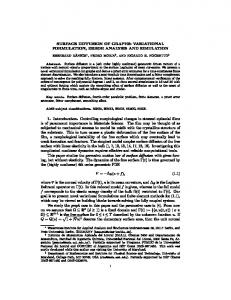
and the claim of the proposition follows due to (5.18). Corollary 5.16. Let the ellipticity and compatibility conditions (1.2) and (5.16) be fulfilled, let AT and BT denote the discrete operators from (1.17) and S = τ AT and T = τ BT , and let R = PL−1 (I + ST )PR−1 be the Left-Right preconditioned system. Then both Richardson and GMRes iterations converge with an asymptotic linear convergence rate. If δ0 is as in Theorem 5.6, the rate is 1 − δ0 in any norm for the former 1− 12 δ0 whereas it is 1+δ in the 2-norm for the latter. 0 Proof. The result is now a simple consequence of Corollaries 5.7 and 5.11 and the above considerations concerning Assumptions 1 and 2. 6. Application to Surface Diffusion. We now discuss the performance of the proposed preconditioners when applied to the nonlinear system (1.4), first linearized via semi-implicit time stepping. We consider the evolution by surface diffusion of the graph plotted in Figure 6.1 (left), with periodic boundary conditions. We use linear finite elements on three nested uniform meshes: 8192 DOFs (h = 2−5 ≈ 0.031),
32768 DOFs (h = 2−6 ≈ 0.016),
131072 DOFs (h = 2−7 ≈ 0.0078). In Figure 6.1 we plot the evolving surface to illustrate that it is rough at the beginning, and slowly regularizes, thereby leading to very high values of q(u) in (1.4), which in turn imply very small values for the coefficient functions a and b in this example. The situation depicted is very similar to the nasty example.
Fig. 6.1. Evolution of an initially rough graph by surface diffusion governed by the system (1.4). Solution at t = 0 (left), t = 0.0005 (middle), t = 0.0010 (right)
In Figure 6.2 we display the number of iterations versus time (for three different time step sizes, respectively) needed for each preconditioner. The performance of the Left Preconditioner, at least in the initial phase of the evolution, where the surface is still rough, is not great. This is caused by the rather big discrepancy of operators S and T due to (locally) high values of q(u). Interestingly, the Right Preconditioner behaves much better in this situation. The behavior of the Left-Right Preconditioner is again striking. The number of iterations is always between 1 and 4, even in the rough initial phase of the evolution. 21
no. of iterations
no. of iterations
no. of iterations
18
160 tau=1e−3 tau=1.e−4 tau=1.e−5
140 120
14
100
12
80
10
60
8
40
6
4
tau=1e−3 tau=1.e−4 tau=1.e−5
16
tau=1e−3 tau=1.e−4 tau=1.e−5
3.5
3
2.5
2
1.5
4
20 0 0
0.005
0.01
2 0
0.015
0.005
0.01
1 0
0.015
0.005
0.01
time
time
0.015
time
Fig. 6.2. Number of iterations versus time for the example of surface diffusion of Fig. 6.1: Left Precondtioner (left), Right Preconditioner (center) and Left-Right Preconditioner (right).
7. Comparisons and Conclusions. The discussion in § 4 and § 5 about the Left and the Left-Right preconditioners indicates that both work well but stops short of displaying which method works best. This is not obvious in terms of condition numbers and spectral radii. Departure p from normality prevents us from estimating theoretically the error reduction rate ρ(Q∗ Q) in the L2 -norm for Richardson’s iteration; see Remark 5.8. Nonetheless, wepinvestigate this issue computationally and find the results displayed ρ(Q∗ Q) is approximately the same as ρ(Q), an amazing fact that in Figure 7.1: deserves further research. L2−error reduction for Richardson for the left/right preconditioner
L2−error reduction for Richardson for the left/right preconditioner
0.7
L2−error reduction for Richardson for the left/right preconditioner
0.7 dim: 161 dim: 705 dim: 2945 dim: 12033
0.6
0.8 dim: 161 dim: 705 dim: 2945 dim: 12033
0.6
0.5
0.5
0.4
0.4
dim: 161 dim: 705 dim: 2945 dim: 12033
0.7 0.6
0.3
rho(S2)
rho(S2)
rho(S2)
0.5
0.3
0.4 0.3
0.2
0.2
0.1
0.1
0 −10 10
−5
10
τ
0
10
0.2 0.1
0 −10 10
5
10
L2−error reduction for Richardson for the left/right preconditioner
−5
10
τ
0
10
0 −10 10
5
10
L2−error reduction for Richardson for the left/right preconditioner
0.7
0.7 dim: 1888 dim: 4203 dim: 6576 dim: 9034
0.6
0.5
0.4
0.4
τ
0
10
5
10
0.8 dim: 789 dim: 2778 dim: 5625 dim: 12337
0.6
0.5
−5
10
L2−error reduction for Richardson for the left/right preconditioner dim: 1782 dim: 4621 dim: 7178 dim: 11590
0.7 0.6
rho(S2)
rho(S2)
rho(S2)
0.5
0.3
0.3
0.4 0.3
0.2
0.2
0.1
0.1
0 −10 10
−5
10
τ
0
10
5
10
0.2 0.1
0 −10 10
Fig. 7.1. L2 –error reduction rate
−5
10
τ
0
10
5
10
0 −10 10
−5
10
τ
0
10
5
10
p
ρ(Q∗ Q) for Richardson’s iteration versus τ for the left/right non-symmetrically preconditioned system. The plots correspond to Examples 2.1–3 with uniform meshes (top) and adaptive meshes (bottom).
We embark now on a more systematic comparison of the performance of the two methods. We examine preconditioned CG (PCG) and GMRes (S-GMRes) for the (symmetric) Left Preconditioner as well as Richardson and GMRes for the (nonsymmetric) Left-Right Preconditioner. Since the overall computational cost is by far dominated by the evaluation of the preconditioned operator, we report on the number of iterations as an indicator of performance. We hereby assume that the cost per evaluation is comparable for both variants of the preconditioner. 22
To this end we chose the forcing functions f = 1, g = 0 in (1.16) and started all iterations with u0T := 0. For a fair comparison we avoid dealing with the stopping tests within MATLAB because they are based on different residual norms for different methods. Instead, we devise an outer loop that terminates at iteration k provided ||ukT − uT ||L2 (Ω) ≤ 1e-7, where uT is a discrete solution obtained by imposing a very sharp stopping criterion to CG. The computational results for the finest partition are displayed in Figure 7.2 (uniform mesh) and Figure 7.3 (graded mesh). For completeness we point out that for coarser meshes the results are essentially the same. Iteration counts
Iteration counts
25
Iteration counts
25 PCG S−GMRES Richardson GMRES
20
45 PCG S−GMRES Richardson GMRES
20
dim of system: 12033
PCG S−GMRES Richardson GMRES
40 35
dim of system: 12033 30
15
15
10
10
25 dim of system: 12033
20 15 5
10
5
5 0 −10 10
−5
10
τ
0
10
5
10
0 −10 10
−5
10
τ
0
10
5
10
0 −10 10
−5
10
τ
0
10
5
10
Fig. 7.2. Number of iterations vs τ for the symmetric and non-symmetric preconditioners on uniform meshes for Examples 2.1–3. Iterative methods: PCG (preconditioned CG) and S-GMRes (GMRes) for the symmetrically preconditioned system; GMRes and Richardson for the non-symmetrically preconditioned system.
Iteration counts
Iteration counts
25
Iteration counts
25 PCG S−GMRES Richardson GMRES
20
45 PCG S−GMRES Richardson GMRES
20
dim of system: 9034
PCG S−GMRES Richardson GMRES
40 35
dim of system: 12337 30
15
15
10
10
25 20 dim of system: 4621 15 5
10
5
5 0 −10 10
−5
10
τ
0
10
5
10
0 −10 10
−5
10
τ
0
10
5
10
0 −10 10
−5
10
τ
0
10
5
10
Fig. 7.3. Number of iterations vs τ for the symmetric and non-symmetric preconditioners on graded meshes for Examples 2.1–3. Iterative methods: PCG (preconditioned CG) and SGMRes (GMRes) for the symmetrically preconditioned system; GMRes and Richardson for the non-symmetrically preconditioned system.
The simulations refer to Examples 2.1-3 of § 2. Our findings are as follows: • For the Left Preconditioner the agreement between computational results of Figure 2.1 and the theoretical upper bound (4.3) is excellent, even though the latter is a bit pessimistic (by a factor 2 in the nasty example): according to (4.3) we have (a) κ ≤ 4,
(b) κ ≤ 8.4,
(c) κ ≤ 86.666.
• Although the three non-symmetric preconditioned systems mentioned at the beginning of § 5.1 possess the same spectra, their performance within, say, a Krylov space method might be different. Our experiments indicate that it is generally better for the Left-Right preconditioned matrix R = PL−1 DPR . The difference in performance 23
• • • •
Spectral radius of Richardson for the left/right preconditioner 1 dim: 161 dim: 705 dim: 2945 0.8 dim: 12033
Uniform grids 1000 dim: 161 dim: 705 dim: 2945 dim: 12033
0.9
700
0.7
0.7
600
0.6
0.6
rho(S)
800
kappa
2
L −error reduction for Richardson for the left/right preconditioner 1 dim: 161 dim: 705 dim: 2945 0.8 dim: 12033
0.9
900
500
rho(S2)
•
increases as the coefficient matrices a and b are more dissimilar, as in Examples 2.3 (nasty) and 2.4 (degenerate). The simple Richardson method is worst in most cases, but only by a small factor of 3–5 in terms of number of iterations. CG and GMRes for the Left Preconditioner behave very similarly. GMRes for the Left-Right preconditioned system achieves the best performance in almost all cases. The comparison is most favorable for the most difficult Examples 2.3 (nasty) and 2.4 (degenerate). The performance of GMRes for the Left-Right preconditioned system is rather robust with respect to the difficulty of the underlying problem. For degenerate operators, the behavior of conditions numbers, spectral radii and thus iteration counts for most of the iterative methods deteriorate; see Figs. 7.4 and 7.5. This is an indication that our assumption on uniform ellipticity is somewhat sharp. Amazingly, GMRes for the Left-Right preconditioned system performs still reasonably well also in this case.
0.5
0.5
400
0.4
300
0.3
0.3
200
0.2
0.2
100
0.1
0 −10 10
−5
10
τ
0
0.1
0 −10 10
5
10
0.4
10
−5
10
0
τ
10
0 −10 10
5
10
−5
τ
10
0
10
5
10
Fig. 7.4. Example 2.4, degenerate case: condition numbers versus τ for the symmetrically preconditioned systems (left); spectral radius ρ(Q) for Richardson’s iteration operator Q forpthe left/right non-symmetrically preconditioned system (middle); L2 –error reduction rate ρ(Q∗ Q) (right); uniform grids.
Iteration counts
Iteration counts
100
180 PCG S−GMRES Richardson GMRES
90 80
PCG S−GMRES Richardson GMRES
160 140
70
120
60
100
50 80
40
60
30
40
dim of system: 705
20
0 −10 10
dim of system: 12033
20
10 −5
10
τ
0
10
0 −10 10
5
10
−5
10
τ
0
10
5
10
Fig. 7.5. Number of iterations vs τ for the symmetric and non-symmetric preconditioners on two different uniform meshes for the degenerate Examples 2.4. Iterative methods: PCG (preconditioned CG) and S-GMRes (GMRes) for the symmetrically preconditioned system; GMRes and Richardson for the non-symmetrically preconditioned system.
• For surface diffusion of graphs, our motivating geometric PDE, the Left-Right preconditioner outperforms the other two; see § 6. On the basis of these experiments, we conclude that it is advisable to use the LeftRight Preconditioner with GMRes, especially when both operators AT and BT differ considerably. This makes use of both operators and exhibits the best performance overall. 24
REFERENCES [1] B. Aksoylu and M. Holst, Optimality of multilevel preconditioners for local mesh refinement in three dimensions, SIAM J. Numer. Anal., 44 (2006), pp. 1005–1025. [2] F. Bai, C.M. Elliott, A. Gardiner, A. Spence, and A.M. Stuart, The viscous CahnHilliard equation. I. Computations, Nonlinearity 8 (1995), 131–160. ¨ nsch, P. Morin, and R.H. Nochetto, Finite element methods for surface diffusion, [3] E. Ba In: P. Colli, C. Verdi, A. Visintin (eds.), Free Boundary Problems. International Series of Num. Math., vol. 147, 53–63, Birkhuser (2003). ¨ nsch, P. Morin, R. H. Nochetto, Surface Diffusion of Graphs: Variational Formula[4] E. Ba tion, Error Analysis, and Simulation. SIAM J. Numer. Anal. 42 (2004), 773–799. ¨ nsch, P. Morin, R. H. Nochetto, Finite element methods for surface diffusion: the [5] E. Ba parametric case. J. Comp. Physics 203 (2005), 321–343. ¨ rnberg, A parametric finite element method for fourth [6] J. Barrett, H. Garcke, and R. Nu order geometric evolution equations, J. Comput. Phys. 222 (2007), 441–467. ¨ rnberg, On the variational approximation of combined [7] J. Barrett, H. Garcke, and R. Nu second and fourth order geometric evolution equations, SIAM J. Sci. Comput. 29 (2007), 1006–1041. ¨ rnberg, Parametric approximation of Willmore flow [8] J.W. Barrett, H. Garcke and R. Nu and related geometric evolution equations, SIAM J. Sci. Comput. 31 (2008), 225–253. [9] J. W. Barrett, R. Nurnberg and V. Styles Finite element approximation of a phase field model for void electromigration, SIAM J. Numer. Anal. 42, (2004), 738–772. [10] S. Bartels, G. Dolzmann, and R.H. Nochetto, A finite element scheme for the evolution of orientational order in fluid membranes Model. Math. Anal. Numer. 44 (2010), 1–32. [11] A.J. Bernoff, A.L. Bertozzi, and T.P. Witelski, Axisymmetric surface diffusion: dynamics and stability of self-similar pinchoff, J. Statist. Phys. 93 (1998), 725–776. [12] A.L. Bertozzi and M.G. Pugh, Long-wave instabilities and saturation in thin film equations, Comm. Pure Appl. Math. 51 (1998), 625–661. [13] J.F. Blowey and C.M. Elliott, The Cahn-Hilliard gradient theory for phase separation with nonsmooth free energy. II. Numerical analysis, European J. Appl. Math. 3 (1992), 147–179. ¨ n, M. Lenz, and M. Rumpf, Numerical methods for fourth order nonlinear [14] J. Becker, G. Gru degenerate diffusion problems, Mathematical theory in fluid mechanics (Paseky, 2001). Appl. Math. 47 (2002), no. 6, 517–543. [15] P. Bjørstad, Fast numerical solution of the biharmonic Dirichlet problem on rectangles, SIAM J. Numer. Anal. 20 (1983), 59–71. [16] P. Bjørstad and B.P. Tjøstheim, Efficient algorithms for solving a fourth-order equation with the spectral-Galerkin method, SIAM J. Sci. Comput. 18 (1997), 621–632. [17] A. Bonito, R.H. Nochetto, and M.S. Pauletti Parametric FEM for geometric biomembranes, J. Comp. Phys. 229 (2010), 3171–3188. [18] F. Bornemann, An adaptive multilevel approach to parabolic problems. III. 2D error estimation and multilevel preconditioning, IMPACT of Computing in Science and Engineering 4 (1992), no. 1, 1–45. [19] D. Braess and P. Peisker, On the numerical solution of the biharmonic equation and the role of squaring matrices for preconditioning, IMA J. Numer. Anal. 6 (1986), 393–404. [20] J. H. Bramble, Multigrid Methods, vol. 294 of Pitman Research Notes in Mathematical Sciences, Longman Scientific & Technical, Essex, England, 1993. [21] J. H. Bramble, J. E. Pasciak, and J. Xu, Parallel multilevel preconditioners, Math. Comp., 55 (1990), pp. 1–22. [22] J. Bramble, J. Pasciak, and P.S. Vassilevski, Computational scales of Sobolev norms with application to preconditioning, Math. Comp. 69 (2000), 463–480. [23] J. H. Bramble and X. Zhang, The analysis of multigrid methods, in Handbook of numerical analysis, Vol. VII, North-Holland, Amsterdam, 2000, pp. 173–415. [24] J.W. Cahn, C.M. Elliott, and A. Novick-Cohen, The Cahn-Hilliard equation with a concentration dependent mobility: motion by minus the Laplacian of the mean curvature, European J. Appl. Math. 7 (1996), 287–301. [25] U. Clarenz, U. Diewald, G. Dziuk, M. Rumpf, and R. Rusu, A finite element method for surface restoration with smooth boundary conditions, Comput. Aided Geom. Design 21 (2004), 427-445. [26] L. Chen and C.-S. Zhang, AFEM@matlab: a Matlab package of adaptive finite element methods, Technique Report, Department of Mathematics, University of Maryland at College Park, (2006). [27] K. Deckelnick, G. Dziuk, and C.M. Elliott, Computation of geometric partial differential 25
equations and mean curvature flow, Acta Numer. 14 (2005), 139–232. [28] Q. Du, A phase field formulation of the Willmore problem, Nonlinearity 18 (2005), 1249-1267. [29] Q. Du and X. Wang, Modelling and simulations of multi-component lipid membranes and open membranes via diffuse interface approaches J. Math. Bio., 2007. [30] Q. Du, M. Li, and C. Liu, Analysis of a phase field Navier-Stokes vesicle-fluid interaction model, Disc. Cont. Dyn. Sys. B, 8 (2007), 539-556. [31] G. Dziuk, An algorithm for evolutionary surfaces, Numer. Math. 58, (1991) 603-611. [32] G. Dziuk, Computational parametric Willmore flow, Numer. Math. 111 (2008), 55–80. [33] C.I. Goldstein, T.A. Manteuffel, S.V. Parter, Preconditioning and Boundary Condtions without H2 Estimates: L2 Condition Numbers and the Distribution of the Singular Values, SIAM J. Numer. Anal. 30, no. 2 (1993), 343–376. [34] G. H. Golub and Ch. van Loan, Matrix computations, 2nd edition, J. Hopkins University Press, (1989). ¨ n, On the convergence of entropy consistent schemes for lubrication type equations in [35] G. Gru multiple space dimensions, Math. Comp. 72 (2003), 1251–1279. ¨ n and M. Rumpf, Nonnegativity preserving convergent schemes for the thin film equa[36] G. Gru tion, Numer. Math. 87 (2000), 113–152. [37] W. Hackbusch, Multigrid Methods and Applications, vol. 4 of Computational Mathematics, Springer–Verlag, Berlin, (1985). [38] M. R. Hanisch, Multigrid preconditioning for mixed finite element methods. PhD thesis. Cornell University (1991). [39] N. L. Nachtigal, S. C. Reddy, and L. N. Trefethen, How fast are nonsymmetric matrix iterations?, SIAM J. Matrix Anal. Appl. 13 (1992), 778–795. [40] P. Oswald, Multilevel Finite Element Approximation, Theory and Applications, Teubner Skripten zur Numerik, Teubner Verlag, Stuttgart, (1994). [41] R.E. Rusu, An algorithm for the elastic flow of surfaces, Interfaces Free Bound. 7 (2005), 229-239. [42] Y. Saad, Iterative Methods for Sparse Linear Systems, Second Edition, SIAM, 2003. [43] A. Schmidt and K. G. Siebert, Design of Adaptive Finite Element Software: The Finite Element Toolbox ALBERTA, Springer LNCSE Series 42 (2005). ´, A black-box multigrid preconditioner for the biharmonic [44] D. Silvester and M.D. Mihajlovic equation, BIT 44 (2004), 151–163. ´, Efficient parallel solvers for the biharmonic equation, [45] D. Silvester and M.D. Mihajlovic Parallel Comput. 30 (2004), 35–55. [46] Y. Song, A note on the variation of the spectrum of an arbitrary matrix, Linear Algebra Appl. 342 (2002), 41–46. [47] L. N. Trefethen and M. Embree, Spectra and pseudospectra. The behavior of nonnormal matrices and operators, Princeton University Press (2005). [48] O. B. Widlund, Some Schwarz methods for symmetric and nonsymmetric elliptic problems, in Fifth International Symposium on Domain Decomposition Methods for Partial Differential Equations, D. E. Keyes, T. F. Chan, G. A. Meurant, J. S. Scroggs, and R. G. Voigt, eds., Philadelphia, 1992, SIAM, 19–36. [49] H. Wu and Z. Chen, Uniform convergence of multigrid v-cycle on adaptively refined finite element meshes for second order elliptic problems, Science in China: Series A Mathematics, 49 (2006), 1–28. [50] J. Xu, Iterative methods by space decomposition and subspace correction, SIAM Review, 34 (1992), 581–613. [51] J. Xu, L. Chen, and R. H. Nochetto, Optimal multilevel methods for H(grad), H(curl), and H(div) systems on graded and unstructured grids, in Multiscale, Nonlinear and Adaptive Approximation, R. DeVore and A. Kunoth eds, Springer (2009),599-659. [52] J. Xu and L. Zikatanov, The method of alternating projections and the method of subspace corrections in Hilbert space, J. Amer. Math. Soc., 15 (2002), 573–597. [53] H. Yserentant, Old and new convergence proofs for multigrid methods, Acta Numer., (1993), 285–326. [54] X. Zhang, Multilevel Schwarz methods, Numer. Math. 63, (1992), 521–539.
26