(C) The input space is divided into 19 regions by the six decision boundaries. The total .... 7 B. Widrow and M. A. Lehr, Proc. IEEE 78, 1415 (1990). ..... In 1982, John Hopfield showed that a network of densely intercon- nected two-state units or ...
610
NUMERICAL COMPUTER METHODS
[29]
predict the pace at which more mathematical knowledge will be embedded in these packages. Acknowledgments This work has been supported by a grant from the Officeof Naval Research.
[29] Artificial N e u r a l N e t w o r k s
By W. T. KATZ,J. W. SNELL, and M. B. MERICKEL Introduction Historically, artificial neural networks have been studied for years in the hope of solving complex real-world problems with humanlike performance. Some appreciation of the magnitude of this task can be obtained by considering the "simple" household fly.l The fly can simultaneously process information from multiple sensors and make complex decisions involving the coordination of a myriad of motor tasks, such as avoiding your fly swatter as it converges on your picnic lunch. This is a particularly impressive task since the neurons of a fly's nervous system have a frequency response of approximately 100 Hz which is 100,000 times slower than the microprocessor components in a home computer. Even today's supercomputers are unable to effectively solve relatively "simple" problems such as the fly scenario presented above. The reasons that biological neural networks have such impressive performance are just beginning to be understood. Modem digital computers built with traditional designs have a fundamental limitation, the so-called von Neumann bottleneck. Traditional computation requires a problem to be broken down to a set of operations which are performed in serial fashion, that is, one instruction at a time. Typically, each instruction must be completed before the next instruction is executed. Artificial neural networks represent a fundamentally different approach to computation. They are explicitly designed to mimic the basic organizational features of biological nervous systems: parallel, distributed processing. It is not surprising then that artificial neural networks (ANNs) have also been called parallel distributed processing, connectionist, and neuromorphic systems. ANNs consist of a large number of simple inter1 j. F. Shepanski, " Q u e s t Technology R e p o r t , " p. 19. TRW Space and Defense Sector, Winter 1987-1988.
METHODS IN ENZYMOLOGY,VOL. 210
Copyright © 1992by Academic Press, Inc. All rightsof reproduction in any formreserved.
[29]
ARTIFICIAL NEURALNETWORKS
611
connected processing elements, where the processing elements are simplified models of neurons and the interconnections between the processing elements are simplified models of the synapses between neurons. Each processing unit or "neuron" can process some piece of information at the same time as other units. The processing of information in such networks therefore occurs in parallel and is distributed throughout each unit composing the network. This approach allows networks of relatively slow, simple processing elements to solve complex, difficult problems with inexact solutions. The rationale behind such a computational model stems in part from the desire to have computers deal gracefully with various real-world problems, namely, situations which require perception and "common sense," two stumbling blocks of the traditional, symbolic approaches to artificial intelligence. Interest in ANNs dates back to at least 50 years ago with some of the early work of investigators in neuroanatomy, neurophysiology, and psychology who were interested in developing models of human learning. An important early model of the biological neuron was proposed in 1943 by McCulloch and Pitts. 2 This McCulloch-Pitts "neuron" is a relatively simple model which assumes the output of the neuron to be binary (i.e., all-or-none) and due to the combined action of inhibitory and excitatory inputs. In this model, the action of inhibitory inputs is absolute such that any inhibitory input completely inhibits the firing of a neuron. In the absence of inhibitory input, the neuron adds all of its excitatory inputs and compares the sum to a threshold to determine whether it should fire. The development of a learning rule which could be used for neural models was pioneered by D. O. Hebb, who proposed the now famous Hebbian model for synaptic modification. 3 This model basically states that the connection (i.e., the synapse) between two neurons is strengthened if one neuron repeatedly participates in firing the other. This Hebbian synaptic modification rule does not express a quantitative relationship between pre- and postsynaptic neurons, and therefore many alternative quantitative interpretations have been developed. However, the Hebbian model for synaptic modification remains important to this day and serves as the reference point for all other learning rules. Rather than tersely cover the breadth of A N N models developed after Hebb's seminal work, this chapter concentrates on two classes of widely used artificial neural networks: the perceptron-back-propagation and the Hopfield-Boltzmann machine models. First, the characteristics of a simple feedforward A N N model is explored in more detail. Then, the per2 W. S. McCulloch and W. Pitts, Bull. Math. Biophys. 5, 115 (1943). 3 D. O. Hebb, "The Organization of Behavior." Wiley, New York, 1949.
612
NUMERICAL COMPUTER METHODS
[29]
X!
x~
X J
W"
FIG. 1. Typical "neuron" or processing unit in an artificial neural network.
ceptron-back-propagation model is presented in an intuitive applicationsoriented style. The chapter concludes with a description of the Hopfield-Boltzmann machine ANN models. Basic Artificial Neural Network Model In Fig. 1, we show the basic structure of the simple processing element or "neuron" in the artificial neural network. The processing unit receives some number of input signals, x ~ , . . . , x n , through weighted links, sums the weighted inputs, and then passes the resulting sum or activation level through an output functionf. The weights on the input lines, w~ . . . . . wn, represent the strength of the connections to a unit, and learning rules (such as the Hebbian rule and the back-propagation algorithm) alter these weights in order to create a desired input/output response from an artificial neural network. In other words, the "knowledge" or functionality of an ANN is encoded in the values of its weights. In many ANNs, the processing units are arranged in layers (Fig. 2). The first layer receives a number of input signals and produces some output which is then fed to the next layer of processing elements, and so on. The input signals constitute some input vector x, whereas the resulting signals from the final or output layer form an output vector y. The cascade of layers can be thought of as a black box which maps input vectors to output vectors. In supervised ANN models, a desired mapping can be obtained by presenting the ANN with training samples, that is, providing the desired output vector Yd for a given input vector x. The ANN then computes
[29]
ARTIFICIAL NEURAL NETWORKS Layer 1
Layer 2
613
Layer 3
Output vector Y = [ Y, Y2]
Input Vector x = [x, x~ x~ ]
FIG. 2. Artificial neural network with its processing units divided into layers.
some measure of the error between the actual and desired output, using a learning algorithm to adjust the weights on the interconnections to reduce the error. Self-organizing ANN models are unsupervised in the sense that no training samples need be provided; the mapping is created after presentation of input vectors only. Therefore, a self-organizing ANN produces similar output vectors when given similar input vectors, the interpretation of "similarity" varying with the particular ANN model. ANN models differ in the manner in which they adjust their weighted interconnections (the learning algorithm), the processing performed by the individual "neurons," and the overall architecture of processing unit interconnection. At the level of the individual processing element, three possible output functions are shown in Fig. 3. The first is linear while the last two are the nonlinear step and sigmoid functions. As mentioned before, each processing unit takes a weighted sum of the input signals and passes this value through the output function. It can be shown that if a linear output function is used, a single layer can be constructed to have f
f 1.0
1.0-
1.0
/
0.5.
0.5
Zwx Linear
f
Zwx Step
S) ~,,wx
Sigmoid
FIG. 3. Linear, step, and sigmoid output functions. The output is plotted against the net input X w x to a processing unit.
614
NUMERICAL COMPUTER METHODS
[29]
FIG. 4. If units with linear output functions are used, multilayer ANNs can be replaced with single layer ANNs.
the same mapping effect as any number of cascaded layers (Fig. 4). Consequently, in order to benefit from additional layers, ANN models usually have nonlinear output functions. Two of the most popular are the step and the sigmoid functions. The Perceptron
Classification Ability of the Perceptron In the late 1950s, Frank Rosenblatt introduced a neural network model called the perceptron, 4 a name which is used for the individual units as well as the overall layered network of units (Fig. 5). The perceptron follows the basic model described above; it accepts inputs through weighted links, sums the inputs, and passes the sum through a step function. The perceptron also has a bias term 0 which serves as a threshold; if the sum from the weighted inputs is greater than - 0 , the unit outputs a " l , " otherwise it outputs a " 0 . " One way of implementing this bias term is to use an additional constant input 1 with its corresponding weight, w0, set to 0. 4 F. Rosenblatt, Psychol. Rev. 65, 386 (1958).
~
1, n e t >_O
"- Y =
O, n e t < 0
net=8+ ~. w~x~
FIG. 5. Perceptron processing unit. Because it uses a hard-limiting step output function, the perceptron gives binary output, " 0 " or " 1 , " depending on the values of the weighted inputs and the threshold term 0.
[29]
ARTIFICIAL NEURAL NETWORKS
615
xe
:XI
x,
F16.6. Decision region of a two-input perceptron. The shaded area, the region above the line xl + x2 = - 1, describes those input values for which the perceptron is " o n " (i.e., gives a " 1 " output).
Despite the simplicity of the model, a perceptron network was shown to be capable of recognizing simple characters as well as other interesting patterns. To get a more intuitive feel for what the perceptron is computing, we will be looking at its processing using geometry. For example, consider a simple case of two inputs and the bias tenn. The input forms a twodimensional input vector, and the space of possible input vectors (the input or feature space) can be shown on a two-dimensional graph. If we map the area for which the perceptron outputs a " 1 , " we find that the border of this " o n " area (the decision region) is formed by a line (the decision boundary) described by the equation XoWo + x l w l = - O . B y varying the values of the weights wo and w 1, we can move the decision boundary and partition the two-dimensional input space into any two parts as long as the parts are linearly separable. And by modifying the sign of the weights, we can choose which side of the decision boundary forms the " o n " area or decision region. A simple example is shown in Fig. 6. We have chosen w0 = 1 and w 1 = 1 with 0 = 1. The decision boundary of this perceptron is a line which runs through (0, - 1) and ( - I, 0); the " o n " area is the region above the
616
NUMERICAL COMPUTER METHODS
[29]
x2
";;~"~'~",,,,~.
- I
-0.5
o.5
~~,~i~ I" X~ - . ";;~'%:'t'~"~i~j~.?.~,.
x~
xe
XOR
0 0 1 1
0 1 0 1
0 1 ! 0
• -0.5
O
-I
•
FIG. 7. The XOR problem. Given two inputs, the perceptron must be " o n " if the two inputs are not identical (filled circles) and " o f f " if the two inputs are identical (empty circles). However, as can be seen, there is no orientation of the decision line which will separate the filled and empty circles.
line. To reverse the labeling, that is, to make the " o n " area the region below the line, we only have to switch the signs of the weights and bias so t h a t w 0 = - l a n d w ~ = -lwith0= -1. The classic XOR problem shows the limitation of a single perceptron (Fig. 7). The XOR (exclusive-or) function is a simple logical function which returns a " 1 " if the two inputs are not identical and a " 0 " if they are identical. As can be seen from simple inspection of the input space, the required mapping cannot be produced by any orientation of a single decision line, that is, it is linearly inseparable. Therefore, the XOR function cannot be implemented by a single perceptron. If more input signals are allowed, the input vector and the corresponding feature space grow in dimensionality. For example, if we have a perceptron with three inputs, the resulting decision boundary is a plane in the three-dimensional feature space. For a perceptron with four or more inputs, the decision regions are bounded by a n-dimensional hyperplane which splits the feature hyperspace. But we return to the two-dimensional case to visualize the mapping ability of multilayer perceptrons. Figure 8 shows some of the decision regions that can be formed by using just three perceptrons in two layers. The first layer consists of two perceptrons which partition the feature space using two decision lines. Each perceptron in this first layer divides the feature space into an " o n " area and an " o f f " area. The weights of the final perceptron can be set so the unit emulates any of a number of logical functions, thereby allowing
[29]
ARTIFICIAL NEURAL NETWORKS
Decision LJne1 ~
617
D~lMon Ilm2
(B) ORed Regions
x
(A) ANDed Regions +1
W'
+1
X2 FIG. 8. Use of a two-layer perceptron with two-dimensional input vectors [xl x2]. Each of the two units in the first layer (numbered 1 and 2) partition the input space into two parts (see Fig. 6). The single unit in the second layer combines these resultant decision regions depending on the connection weights between the first and second layer. (A) The final unit implements an " A N D " function, and the final output of the two-layer perceptron is the intersection between the t w o " o n " areas of the first-layer units. (B) The final unit implements an " O R " function, and the final decision region is the union of the two " o n " areas of the first-layer units.
the combination of decision regions resulting from the first layer. Thus, the intersection of the two " o n " areas can be obtained by setting the weights so that the final perceptron acts as an " A N D " unit. Alternatively, the union of the " o n " areas can be found by using the perceptron as an " O R " unit. By increasing the number of units in the first layer, we can add edges to our decision boundary and create more complex decision regions. In fact, we can come arbitrarily close to making a decision region for any convex and many concave connected areas, bounded or unbounded. Figure 9 provides an example of how a complex nonconvex decision region can be formed using a two-layer perceptron. The six units in the first layer divide the two-dimensional feature space into 19 different regions with their six decision lines. The perceptron in the final layer selects those areas which lie in at least four " o n " regions. The resulting decision region is quite complex despite the use of only 7 perceptrons. The next step in our geometric analysis is to add a final layer to form a three-layer perceptron. The perceptron in the final layer can combine the results from several units in the second layer, and in so doing, extend a decision region to incorporate disjoint areas of arbitrary shape in the
618
NUMERICAL COMPUTER METHODS
+I
[29]
+I
3 4
4
3
(,4) ANN Structure
(B) ANN Decision Region
(C) Map Of "ON" Regions
F~G. 9. Formation of a complex nonconvex decision region using a two-layer perceptron with six units in the first layer and a single second layer unit. (A) The perceptron architecture. (B) The output decision region (shaded). Each numbered line corresponds to the decision boundary for the identically numbered unit in the first layer. Even-numbered units have their " o n " regions covering the origin, whereas odd-numbered units have their " o n " regions facing away from the origin. (C) The input space is divided into 19 regions by the six decision boundaries. The total number of first-layer units which are " o n " in each region is shown. Note that the output decision region in (B) corresponds to regions which have four or more " o n " units.
input space. In the example shown in Fig. 10, a triangular donut is formed by subtracting a smaller triangular area from a larger region. There are two conclusions which can be drawn from our geometric analysis of the simple two-dimensional case. First, three layers are sufficient to represent any decision regions, provided they consist of a finite number of disjoint areas: Second, a priori information regarding the complexity of the desired decision region can directly influence the required number of units in each network layer. For example, if we are using twodimensional input vectors, and it is known that the desired decision region consists of two disjoint areas, we will probably need at least six units in the first layer and two units in the second layer. Closed boundaries in twodimensional space require a minimum of three sides (a triangle); therefore, two sets (for the two disjoint areas) of three units are required in the first layer. An additional two units are required in the second layer to combine (via " A N D , " " O R , " or other boolean functions) the first layer results and create the disjoint decision regions. This example can be extrapolated to a general heuristic: a minimum of m(n + l) first layer perceptrons and rn second layer perceptrons are needed to construct a decision region encompassing rn disjoint areas in a n-dimensional feature space. 5 G. J. Gibson and C. F. N. Cowan, Proc. 1EEE 78, 1590 (1990).
[29]
ARTIFICIAL NEURAL NETWORKS
619
X2
+1
XI
(A) ANN Structure
(B) ANN Decision Region
FIG. 10. Decision region formed by a three-layer perceptron. (A) The six first-layer units form six decision lines in the input space. The first three (1-3) form the sides of the outer triangle, and the second three (4-6) form the sides of the smaller inner triangle. The "on" areas for all six units face the interior of the triangles, so the "AND" units in the second layer form triangular decision regions. The single third-layer unit subtracts the inner triangle from the outer triangle to form the finaltriangular donut decision region. (B) The finaldecision region (shaded) is shown with the numbered edges corresponding to the decision lines of identically numbered first-layer units shown in (A).
Perceptron Learning Algorithm In the previous section, we analyzed the types of decision regions which could be represented by multilayer perceptrons. Although a threelayer p e r c e p t r o n can generate arbitrarily complex decision regions, in the 1950s there were no known ways in which to adaptively set the weights in these multilayer networks given a training set of input vectors and the corresponding desired outputs. There were, however, methods for learning the weights for a one-layer perceptron. Rosenblatt published the perceptron learning theorem which gave both a learning algorithm and a proof that any decision region that could be represented by a single layer perceptron could be learned using his learning algorithm. As we have seen in the section above, single-layer perceptrons can represent (and therefore learn by the perceptron learning theorem) any linearly separable decision regions. Unfortunately, if presented with nonlinearly separable problems, the perceptron learning algorithm may continue to oscillate between the decision boundaries indefinitely.
620
NUMERICAL COMPUTER METHODS
[29]
Shortly after Rosenblatt's perceptron learning rule was presented, Widrow and Hoffindependently introduced the least mean squares (LMS) or Widrow-Hoff delta (8) rule.6'7 This algorithm attempts to minimize the mean squared error between the desired and actual output. Whereas the LMS method is not guaranteed to separate linearly separable classes, it will converge on reasonable decision boundaries in linearly inseparable problems. L M S or W i d r o w - H o f f D e l t a R u l e
0. Initialize the weights and bias terms to small random values. 1. Compute the net input, n e t = E w x , to each perceptron unit using some input vector x from the training set. 2. Calculate the error, 8 = d - n e t , where d is the desired output. 3. Adjust each of the weights of the unit in proportion to the error and the input signal coming in over that line. The change in weight wi is given by the equation hw i = aSxi where a is a learning rate or gain term (usually set to the range 0.1 < a < 1.0) controlling the stability and speed of convergence to the correct weight values. 4. Go to Step 1. The key difference between the perceptron and LMS training algorithms is in Step 1: the perceptron learning algorithm passes the weighted sum of inputs, net, through the output step function so that 8 = d - y where y = f ( n e t ) as in Fig. 5. In other words, the perceptron learning algorithm uses the actual unit output y, whereas the LMS algorithm uses the net input in the derivation of the error term. This means that the adaptation of weights can continue (Awi ~ 0) in the LMS case even if the actual output agrees with the desired output. In human learning, such continual adaptation is typical as in the case of medical problem solving. For example, first-year medical students may correctly make a diagnosis (y = d) although they lack confidence in their judgment (8 ~ 0). On the other hand, trained clinicians with repeated exposure to a number of similar cases can make the same diagnosis more rapidly and with more certainty (smaller 8). The perceptron and LMS learning procedures work for a single layer perceptron. But what about the multilayer perceptron? In this case, the weights for the final layer can be modified because the error 8 between the final layer and the desired outputs can still be computed. But the adjustment for weights in "hidden" layers (i.e., all layers but the final one) are 6 B. Widrow and M. E. HolT, "1960 IRE WESCON Convention Record," p. 96. IRE, New York, 1960. 7 B. Widrow and M. A. Lehr, Proc. IEEE 78, 1415 (1990).
[29]
ARTIFICIAL NEURAL NETWORKS
621
r
X3
"
A,#
1
y= 1+
e ~"
n e t = e + ~ w, x, 1.1
X~ ~ W ~ FI6. 11. " N e u r o n " or processing unit in the back-propagation ANN.
not so easily computed since there is no direct error measurement 8 between a hidden layer units and the given desired output. Back-propagation
Network and Geometry of Decision Regions The training of multilayer neural networks proved to be a thorny problem. Without the prerequisite learning algorithm, training was limited to single layer perceptrons with all of the inherent limitations in representing only linearly separable decision regions. It was no surprise, then, that the introduction of the back-propagation algorithm in the 1980s proved a great boon to the fledgling artificial neural network movement. Backpropagation or "backprop" is a simple, easily implemented training algorithm for multilayer feedforward networks, s The units in the backprop network are identical to perceptrons except for the replacement of the step output function with a sigmoid function (Fig. I 1). The sigmoid is used because the error measurements require the output function to be differentiable. The conclusions obtained from the geometric analysis of the perceptron can be extended to the back-propagation ANN model. The use of the sigmoid as the output function complicates the geometric analysis, but the overall results are similar. Instead of lines, planes, and hyperplanes forming the decision boundaries, the sigmoid output function generates curves, s D. E. Rumelhart, G. E. Hinton, and R. J. Williams, "Parallel Distributed Processing," p. 318. MIT Press, Cambridge, Massachusetts, 1986.
622
NUMERICAL COMPUTER METHODS
[29]
curved surfaces, and hypersurfaces which form the decision boundaries. One caveat should be given regarding the theoretical analysis of minimum ANN requirements. As mentioned in the discussion of perceptrons, a three-layer ANN can represent any arbitrarily complex decision region. However, it may be advisable to use more than three layers, because in practice, the size (number of hidden units) and training time requirements of a minimal three-layer network may be much greater than that of a network consisting of more layers. Back-propagation Learning Algorithm Back-propagation Learning Algorithm
0. Initialize the weights and bias terms to small random values (e.g., - 0 . 5 to 0.5). 1. Compute the actual output vector y by propagating some input vector x from the training set forward through each layer. 2. Start at the output layer and calculate the error 8i = y/(1 - y;) (d, - Yi), where 8i is the error term for output unit i, y/is the output for unit i (the ith component of the output vector y), and d; is the desired output for unit i. The (di - Yi) term relates the magnitude of the error while the remaining terms are the derivative of the sigmoid output function. 3. Adjust each of the weights of the output units in proportion to the error and the input signal coming in over that line. The change in weight w/is given by the equation Aw/= aSix/where o~is a learning rate or gain term (usually set to the range 0.1 < a < 1.0) controlling the stability and speed of convergence to the correct weight values. 4. After completing the weight changes for the output layer, work backward layer by layer to the first hidden layer. At each layer: 4a, Calculate the error ~i :
Xi(1 -- Xi) ~ ~jWij J
where 8~ is the error term for unit i of the current layer, x i is the output for unit i, 8j is the error term for unitj in the layer after the current layer, and w o. is the weight between unit i and unit j. The sum in the error term basically back-propagates the errors from the units j to which the current unit i is connected. 4b. Adjust the weights (as in Step 3) leading to unit i using the 8i calculated in Step 4a. 5. Go to Step I. Note that the only difference between the back-propagation and LMS
[29]
ARTIFICIAL NEURAL NETWORKS
623
i ....
(2 "~-. ". "'4
Training set
...,::::.?.:.,:; ,,::~z:~..-.-{i~...~-.."
.2 Movement with Training
Training Time /}.
B
FXG. 12. Generalization degradation due to overtraining. (A) Decision lines move closer to training points (large triangles) during training. Possible test input points in the same class (small points) are distributed over a larger area. As the decision lines move closer to the training points, they may pass over the test input points. (B) The result is an eventual degradation of test point classification even though performance on the training set continues to rise.
learning algorithms is the definition of the error term 8. In LMS, the error term was simply the difference between the actual output and the sum of weighted inputs. In backprop, we have two different 8 terms (Steps 2 and 4 above) depending on whether the unit is in a hidden layer or output layer. The back-propagation procedure can require thousands of presentations of each input and desired output vector pair in the training set. To speed the process, a momentum term can be added to the weight change (Step 3). Then, the change in weight is A w i = o t ~ i x i + ~ A w i ( n - 1) where is the momentum (usually less than 0.9) and A w i ( r l - 1) is the weight change from the previous training input. Overtraining
It is possible to overtrain an artificial neural network so that it generalizes poorly to novel input vectors. This problem can be seen geometrically (Fig. 12). The training set is a sample from the set of all possible input/ output vector pairs. If training on the samples continues for too long, the ANN will move its decision boundaries arbitrarily close to the sample points. Also, if too many units are used in the network relative to the number of samples in the training set, the ANN may "memorize" the samples by forming tight, disjoint decision regions around each sample point. In either case, the resultant decision regions will exclude input
624
NUMERICAL COMPUTER METHODS
[29]
vectors similar to those in the training set: generalization will be poor. One method of preventing overtraining is simply to halt training as soon as all training samples are correctly identified rather than trying to obtain zero error or training for a predetermined number of passes.
Error Surfaces Learning algorithms attempt to find some set of weight values which produce the desired mapping (or, in geometric terms, represent the required decision regions). If we had n connection weights in a neural network, we could think of an (n + 1)-dimensional space with n axes corresponding to the different weights and one axis representing the overall error between desired and actual outputs. 9 In this space, we could describe an error surface giving the error for each possible combination of weights. The back-propagation learning algorithm implements a form of gradient descent on this error surface. It changes the weight values in such a manner as to follow the error surface slope downward to a minimum. Usually, the error surface is highly convoluted with many areas of shallow slope (owing to the small effect of weight changes when unit outputs are very large), pockets of varying depth (local minima), and possibly many equally deep holes (global minima). By following the steepest descent, it is possible that back-propagation could get stuck in one of the local minima or progress with extreme slowness through relatively flat terrain. Although the latter scenario (slow convergence) may be prevalent in many real-world applications, the local minima problem is rarely encountered, and a good minimum, if not a global minima, is usually discovered. Extensions of the backprop learning algorithm have been developed specifically to combat the slowness of training.~°
Back-propagation Applications The back-propagation algorithm has been applied extensively, covering a gamut of problems from backgammon playing to medical diagnosis. In each case, the researcher has (I) chosen a suitable encoding scheme for the problem at hand, (2) specified the number of units and layers as well as the interconnection pattern, and (3) acquired a good training set. The first task is to choose a suitable encoding scheme so that one can represent the requisite information in a form suitable for ANN processing. Therefore, we need to transform our inputs and desired responses into 9 R. Hecht-Nielsen, "Neurocomputing," p. 128. Addison-Wesley, Reading, Massachusetts, 1990. l0 R. A. Jacobs, Neural Networks 1, 295 (1988).
[29]
ARTIFICIAL NEURAL NETWORKS
ALA
~
625
f0 . 0
I PRO
~
0.05
~
0. i 0
~
0.40
~
0.0
I GLU
I SER
I ALA
•
Input Sequence
.]
t
Input Vector
FIG. 13. One method for representing amino acid sequences as numerical vectors. Each residue position corresponds to one component of the input vector, and the types of amino acids are mapped to unique numbers (e.g., ALA = 0.0, PRO = 0.05).
numerical input and output vectors. For example, suppose we want to start with a sequence of amino acids and map this sequence into secondary structure information (a helix, fl sheet, or coil). How would we represent the input (the sequence of amino acids) and the output (the secondary structure) in numerical terms? One possible input representation is to assign a number to each amino acid: alanine would be represented by 0.0, proline by 0.05, glutamate by 0.10, etc. Then, a single input value (i.e., one component of the input vector) could represent one amino acid position in the sequence (Fig. 13). Likewise, the secondary structure types could be assigned values so that a helix is represented by 0.0,/3 sheet by 0.5, and coil by 1.0. Using this type of encoding, the ANN would receive a ndimensional input vector where n is the number of amino acids in the sequence to be input. The ANN output would be a single value corresponding to a type of secondary structure. Although this encoding scheme transforms the training information to numerical vectors efficiently, it is likely that the ANN will be unable to perform a useful mapping because our input and output representations do not mirror the real world. For example, one wo,:ld expect the biological properties of proline to be a similar to alanine since their encodings, 0.0 and 0.05, are very close numerically. In reality, proline is an atypical amino acid that tends to be an a-helix breaker. This property of proline will be difficult to encode using any such "analog" encoding scheme. An alternative encoding scheme uses "local" representation, a form of binary representation. In this scheme, each component of the input
626
NUMERICAL COMPUTER METHODS
[29]
vector represents a particular amino acid; therefore, if we only had to deal with 5 amino acids (instead of the 20 in nature), one position in the sequence could be represented by a five-dimensional input vector. For example, (1 0 0 0 0) could represent proline while (0 1 0 0 0) could represent alanine. This form of representation allows the ANN greater differentiation among the various amino acids. However, this type of encoding requires a 5n-dimensional input vector where n is the number of amino acids in the sequence to be input. The same type of encoding can be used for the output vector. With local representation, we use a threedimensional output vector (produced by 3 units in the output layer) to signify the secondary structure type. An output of (1 0 0) indicates a helix while the vector (0 1 0) indicates/3 sheet. The encoding scheme can greatly influence the success of an ANN application) 1 NETtalk. In 1987, Sejnowski and Rosenberg described a back-propagation application which converted English text into intelligible speech) 2 This application demonstrated the power of ANNs and accelerated the use of the back-propagation algorithm in particular. Sejnowski and Rosenberg organized their ANN into two layers, a hidden and output layer, that accepted a group of sequential letters and output the phonetic symbol corresponding to the central letter. The input and output data were encoded using local representation. By using additional equipment, the researchers were able to convert the ANN output phonetic symbols into sounds. Initially, the ANN "speech" is like baby babble, but as training progresses, words become properly enunciated. Protein Secondary Structure Prediction. Shortly after the NETtalk publication, two independent groups, Qian and Sejnowski 13 and Holley and Karplus, TM applied a similar ANN architecture to the problem of protein secondary structure prediction, replacing the input string of letters with amino acids and the output phonetic symbols with secondary structural types. The researchers obtained a training set of primary and secondary structure information derived from known protein structures listed in the Brookhaven National Laboratory Protein Data Bank. A test set of protein segments was created after removal of candidate proteins with homologies in the training set. As shown in Fig. 14, the ANN receives an input vector representing a segment of primary amino acid sequence. Because the encoding scheme uses local representation, the input vector is a 21n-dimensional vector 11 p. p. 12 T. 13 N. 14 L.
j. B. Hancock, "Proceedings of the 1988 Connectionist Models Summer School," 11. Morgan Kaufmann, San Mateo, California, 1989. J. Sejnowski and R. R. Rosenberg, Complex Syst. 1, 145 (1987). Qian and T. J. Sejnowski, Mol. Biol. 202, 865 (1988). H. Holley and M. Karplus, Proc. Natl. Acad. Sci. U.S.A. 86, 152 (1989).
[29]
ARTIFICIAL NEURAL NETWORKS
/
NH2 •
THR SER ALA ALA ASN TYR CYS
.~
/ ..** ,-"
a~..
ME T
a helix
***
ARG I%%
L¥ As.S I./" ".. LZO l " T"R /
•-Ys/
ASP ARG
o,~
.."
.~ sza~ :~
627
| |
LYs MET |
PRO v.~L
v ~
13sheet i
COil
%" "°.
%++
O"I
Network
COOH Input Sequence
17x21-dimensional Input Vector
FIG. 14. Protein secondary structure prediction using an ANN. A small number of contiguous amino acids are transformed to an input vector. To reduce the complexity of the diagram, only the input vector components corresponding to the central residue position (SER in this case) are shown. The input vector is fed through the ANN, and the output units give the likelihood of the three secondary structure types.
where n is the number of positions (usually 13 to 17) in the amino acid segment. (There are 21 different inputs at each segment position: 20 amino acids and 1 spacer.) After propagating the input vector through the layers, the A N N outputs a vector giving the secondary structure type (a helix,/3 sheet, or coil) of the amino acid at the center of the input segment. This result is compared to the actual secondary structure determined through atomic coordinate analysis using the method of Kabsch and Sander. 15 Errors are used to correct the weights in the ANN via the back-propagation algorithm. Both research groups had similar findings: predictive accuracy was approximately 63% on test proteins nonhomologous with proteins used in the training set. This result indicated that the ANN approach was more accurate than many other methods. An analysis of the trained ANN 15W. Kabsch and C. Sander, Biopolymers 22, 2577 (1983).
628
NUMERICAL COMPUTER METHODS
[29]
showed that the network weights had indeed captured a number of realworld properties. For example, weights connecting "proline" components of the input vector with the " a helix" output unit were strongly negative, correctly indicating that proline tends to prevent o~-helix formation. (Note that use of the encoding scheme in Fig. 13 would hinder the weight representation of the antihelix property of proline.)
Hopfield Networks and Boltzmann Machine Introduction to Optimization Problem
There are many tasks in science and engineering which are referred to as optimization problems, that is, problems that have many valid solutions, but one or more of these solutions is considered to be best. The search for an optimum solution is often a difficult and time-consuming task. The game of chess is an example. If you are the white, there are a number of play sequences leading to the optimum solution: the eventual capture of the black king. But brute force evaluation of all valid moves is computationally intractable owing to the combinatorial explosion of possible lines of play. Conventional approaches to solving optimization problems (e.g., random search or gradient descent techniques) are often slow and yield poor solutions. It is obvious that biological systems rapidly solve these types of problems with a high degree of success. Besides higher cognitive functions like game playing, many routine tasks can be considered optimization problems. Such tasks include the construction of depth field from two monocular scenes by the visual system, finding the proper orientation of the arm for grasping an object given a set of impeding obstacles, and the rapid recognition of a familiar face or object. The Hopfield and Boltzmann models are neurally inspired computational techniques which attempt to deal effectively with optimization problems. Two-State Neuron Model
In 1982, John Hopfield showed that a network of densely interconnected two-state units or "neurons" can exhibit emergent collective computational properties. 16 These networks differ from the perceptron/backprop ANN models in that each neuron is potentially connected to every other neuron; therefore, cycles in the network may form. The resulting feedback endows the ANN with dynamic properties and may prevent the network from reaching a stable state. 16j. Hopfield, Proc. Natl. Acad. Sci. U.S.A. 79, 2554 (1982).
[29]
ARTIFICIAL NEURAL NETWORKS
(i O)
629
(1 1 1)
\
) '010)
y,
(1 oo)
a
Hopfield
Network
\ (ooo) B
(ool) Possible
States
FIG. 15. Three-unit Hopfield network and its possible output states.
Each unit in the Hopfield network is essentially a perceptron with zero threshold, 0 = 0 (see Fig. 5). It sums the weighted inputs and then outputs a " 0 " if the result is negative or " I " if the result is greater than or equal to zero. The network is updated asynchronously. Each neuron randomly and independently evaluates its inputs and updates its output signal. This is very different from the systematic layer-by-layer evaluation of units using the back-propagation algorithm. At any time, the state of the network is defined by the collection of unit outputs, the output vector. Because each unit in the network can be in only two states, " 0 " or " 1 , " the output vector can be thought to represent a vertex of a n-dimensional hypercube, where n is the number of units comprising the network. Figure 15 shows a Hopfield network with three units and the possible values of its output vector. Initially, a Hopfield network is in a state corresponding to some vertex in the n-dimensional hypercube. As each unit evaluates its input and updates its output,the output vector can change by only one component value. Graphically, this means that the point on the hypercube corresponding to the network state can travel only one edge during a single unit update. As time elapses and the output vector changes, the network state can be described by a point moving along the edges of the hypercube. One of the most interesting aspects of Hopfield's paper was its description of the energy (E) of the network state:
630
NUMERICAL COMPUTER METHODS
[29]
B
Network Output State FIG. 16. "Energy" surface of a Hopfield network. The ball represents the output state of the network. As time progresses, the ANN moves from an initial state to either a local minimum (A) or a global minimum (B).
where we is the connection weight between units i and j, and Yi is the output of unit i. The result of each unit update is to lower the overall energy of the network. This can be seen by considering the change in energy due to the change in the output of a single unit: A E = ay,
wijY2 j#i
The summation (net input) and Ayi in the equation are either both positive or negative since the output yi of a unit depends on the sign of the net input; therefore, the energy of the network state is always decreasing. Depending on the values of the connection weights, some vertices of the hypercube will have lower energy than other vertices. So as the state of the system evolves, the output vector will settle onto one of the vertices. This stable state is reached when all of the edges, along which the network state can move, lead to vertices with higher energy. It has been shown that a network comprised of two-state units will eventually reach a stable, fixed state if the connection weights between any two units are identical (i.e., symmetric connections) and no unit excites or inhibits itself. The state which is eventually reached may be a local minimum instead of a global minimum (Fig. 16). Even though some vertex and its corresponding network state has the smallest energy value, the current network state may not be able to reach that global minimum because it first runs into a local minimum. The initial state of the network decides which of the minima the network will eventually settle into.
[29]
ARTIFICIAL NEURAL NETWORKS
631
f
f 1.0
1.0
0.5
_f ~WX
(A) Back-propagation
(B) G r a d e d
response
Hopfield network FIG. 17. The sigmoid used in back-propagation (A) allows output from 0 to 1 while the sigmoid used in graded response Hopfield networks (B) allows output from - 1 to 1.
Graded Response Neurons In 1984, Hopfield replaced the two-state units of the network with continuous output units like those in the back-propagation model. 17 The only difference between the back-propagation unit and Hopfield's graded response unit is the nature of the output sigmoid function (Fig. 17). In the Hopfield model, the output of the sigmoid changes sign when the net input equals zero. This adjustment is necessary to ensure that the energy of the network state always decreases. The graded response of the units allows the output vector components to be continuous values. Therefore, the point corresponding to the network state can lie in the interior of the hypercube, and the constraint of traveling along the hypercube edges is removed. This freedom of movement makes it less likely (although not impossible) that the network state will fall into a local minimum.
Boltzmann Machine: Simulated Annealing In an effort to avoid local minima, a number of researchers began to experiment with the technique of simulated annealing. 18'19 Simulated annealing describes a process similar to the annealing of metal. First, the 17 j. Hopfield, Proc. Natl. Acad. Sci. U.S.A. 81, 3088 (1984). 18 S. Kirkpatrick, C. D. Gelatt, Jr., and M. P. Vecchi, Science 22,0, 671 (1983). 19 S. Geman and D. Geman, IEEE Trans. Pattern Anal. Machine Intelligence 6, 721 (1984).
632
NUMERICALCOMPUTERMETHODS
101
[29]
P
0.5 ~
0.0
FIG. 18. Effectof temperature T on the probabilitythat a unit in the Boltzmannmachine will becomeactive. As T approaches absolute zero, the sigmoidapproachesa step function. At highertemperatures, the sigmoidbecomes flatter,and net input becomesless of a factor in determiningwhether a unit becomes active.
metal is heated to high temperatures, agitating the atoms. Then, as the metal is slowly cooled, the atoms become less agitated and the metal eventually falls into a low energy state. In the case of Hopfield networks, a temperature term T was added to the sigmoid output function and the output function was made probabilistic instead of deterministic (Fig. 18). The probability Pi that a given unit is activated (i.e., it gets turned on with output "1") is given by 1 Pi-
1 d- e net/T
where neti is the sum of weighted inputs. At high temperatures, each unit has a similar chance of being activated regardless of its input. Then, the network is allowed to iterate while the temperature is slowly reduced. At some low temperature, the network output vector will "freeze" to a final, unchanging state. This procedure prevents the network from being trapped in a local minimum since there is always a finite probability of assuming a higher energy state than the current one. In fact, convergence of the system to
[29]
ARTIFICIAL NEURAL NETWORKS
633
the global minimum is guaranteed as long as the temperature is reduced slowly enough. However, the cooling time is not necessarily finite. Simulated annealing can be described graphically with the help of Fig. 16. Initially, the high temperatures can be thought of as violently shaking the state of the network so the state has an equal probability of falling in either well. As the agitation decreases, the probability of the state being in well B (the global minimum) begins to exceed that for well A. The state may jump from A to B, but it is less likely that a jump from B to A is possible since this represents a greater energy difference. Eventually, the state becomes trapped in the desired global minimum and is unable to jump back to the local minimum.
Setting Weights of Hopfield-Boltzmann Machine Artificial Neural Network To solve a particular problem, a researcher must determine appropriate values of the connection weights so that the stable states of the network correspond to desired memories or valid solutions. Whereas the perceptron and back-propagation ANN models were rooted in clearly defined weight learning algorithms, the Hopfield-Boltzmann machine ANNs models rely more on the ability of the researcher to translate a problem into a suitable energy function so that low energy states correspond to optimal solutions of the problem. A brief overview of techniques for weight setting is provided below. Content-Addressable (Associative) Memories. Associative memories are capable of recalling a complete memory given a noisy or incomplete input pattern. This is characteristic of human memory and is extremely useful in pattern recognition applications. Typical computer memory is dependent on knowledge of particular storage locations rather than what is actually stored in those locations. Associative memories, on the other hand, retrieve information by content rather than by location. Recurrent networks, such as the Hopfield networks, can implement these associative memories. If the correct set of weights is used, the network will output a complete desired memory given an incomplete or distorted input. In terms of energy states, the stored memories correspond to ANN states which are local or global minima. With incomplete or distorted input, the ANN starts in a high energy state and, with time, changes its output to the nearest low energy state which hopefully corresponds to the completed input pattern. Given a set of binary encoded memories to be stored, the appropriate values for the weights are given by the following relation:
WU= ~ Yi,pYj,p p=l
634
NUMERICAL COMPUTER METHODS
[29l
where wUis the weight between units i and j, m is the number of memories to be stored, and Yi,p is the desired output of unit i for memory p. To retrieve a memory, the network output is clamped to an input pattern. The output of the network is then freed and allowed to iterate into a low energy state. The resulting output will be the corresponding memory. Associative memories simply find the nearest local minima to a given initial state. There are many situations in which the global minima is desired. This is the case with optimization problems. Here the determination of the connection weights is not nearly as straightforward as that for the associative memory problem. The constraints involved in the optimization must be mapped onto the energy function for the network. An Optimization Problem. The traveling salesman problem (TSP) involves finding an optimum tour between a group of cities. The optimum tour is the shortest tour which visits each city only once and returns to the starting city. If there are n cities, then the number of possible valid tours is given by n!/(2n). Obviously, for problems of more than a small number of cities, exhaustive search for the optimum tour is computationally intractable. This problem can be mapped to a network by constructing an energy function which has minima for all valid tours. 2° These minima will have depths inversely proportional to the length of the tour they represent. As a result, a network with this energy function will tend to settle into one of the deeper minima, namely, a tour solution with minimal distance. An optimum solution is not guaranteed, but acceptable solutions are rapidly achieved. Each city in an n-city tour is represented by a row of n units. Each unit in the row represents the order in the tour in which that city is visited. Therefore, a matrix of n x n units is formed to represent the entire tour (Fig. 19). Note that we reference each unit's output, Yxi, in the ANN by two indices; the first designates the Xth city, whereas the second designates the position of the Xth city on the tour. For example, Y32, is the output from the unit associated with the hypothesis "City 3 is the second city in the tour." We can devise a suitable energy function by considering (1) the constraints on valid solutions and (2) the criteria for " b e s t " solutions. With regard to solution validity, there are two constraints. A city can only be visited once per tour; therefore, only one unit per row must be active. Because only one city can be visited at a time, only one unit per column must be active. Besides validity, we must also incorporate some measure of the goodness of the solution. In the case of the TSP, the total distance 2o j. j. Hopfield and D. W. Tank, Biol. Cybernetics 52, 141 (1985).
[29]
ARTIFICIAL NEURAL NETWORKS
Position 1
city I city 2 city 3 city 4 city ~ city 6
2
3
635
in tour 4
5
6
0 © 0 0 0 0
@0 0 0 0 0 0 0 0 0 0 @ 0 0 ® 0 0 0 0 0 0 0 © 0 0 0 0 ® 0 0
FIG. 19. Hopfield network solution to a six-city traveling salesman problem. Active units (shaded circles) describe a tour solution. The solution pictured in the diagram is a tour with visits to the cities 2, 1, 4, 6, 5, and 3, in that order. Each row represents a city while each column represents a position in the tour. All units are fully connected to each other.
required by a valid solution is the measure we must minimize. The following energy function satisfies all of these conditions:
E= A ~
X
+ D
i j#i
YxiYxj + B ~,~, E
~f'~ ~ i x Y#X
i
dxyyxi(~Y(i_
X Y#X
(
YxiYYi+ C - n +
•
Yxi
1) + yy(i+ 1))
where A, B, C, and D are some large constant values, n is the number of cities in a tour, Yxi is the output of the unit associated with the hypothesis "City X is the ith visit on the tour," and dxr is the distance between city X and city Y. The first two summations (A and B term) are zero only when there is a single active neuron in each row and column, respectively. The third summation (C term) is zero only when there are n active neurons. The fourth term is proportional to the tour length. By relating the above TSP energy function to the general energy function (i.e., E = a ~ , wijyiyj), we can work out the required values for the connection weights between the ANN units. In this case, the weight between any two units is negative and proportional to the distance between the two cities they represent. The weights also include negative contributions from the validity constraints (A, B, and C terms in the energy function). Boltzmann Machine Learning Algorithm. In addition to the two methods given above for the determination of the weights, Sejnowski and coworkers have developed a supervised training method for the Boltzmann
636
NUMERICAL COMPUTER METHODS
[30]
machine ANN. 21,22 Although this method automatically configures the ANN weights for a particular problem, the learning algorithm tends to be extremely slow. Discussion Artificial neural networks are novel, robust computational tools for pattern recognition, data mapping, and other applications. The demonstrated success of ANN techniques has lead to an explosion of interest among scientific and engineering circles. In contrast to the paucity of introductory material a decade ago, ANN texts and journals are now readily available. Both commercial and public domain ANN software exists for a variety of computer systems ranging from small personal computers to large, massively parallel supercomputers. With these instructional and developmental resources, researchers are now able to apply ANNs to a wide range of scientific and engineering problems. 21 D. H. Ackley, G. E. Hinton, and T. J. Sejnowski, Cognit. Sci. 9, 147 (1985). 22 G. E. Hinton and T. J. Sejnowski, "Parallel Distributed P r o c e s s i n g , " p. 282. M I T Press, Cambridge, M a s s a c h u s e t t s , 1986.
[30] F r a c t a l A p p l i c a t i o n s in Biology: S c a l i n g T i m e in Biochemical Networks
By F. EUGENE YATES Introduction
Aims of This Chapter The purpose of this chapter is to present to a readership of biochemists, molecular biologists, and cell physiologists some of the terms and concepts of modern dynamical systems theory, including chaotic dynamics and fractals, with suggested applications. Although chaos and fractals are different concepts that should not be confounded, they intersect in the field of modern nonlinear dynamics. For example, models of chaotic dynamics have demonstrated that complex systems can be globally stable even though locally unstable and that the global stability reveals itself through the confinement of the motion of the system to a "strange attractor" with a microscopic fractal geometry. Some of the technical asMETHODS IN ENZYMOLOGY,VOL. 210
Copyright © 1992by AcademicPress, Inc. All rights of reproduction in any form reserved.