Predicting Australian Stock Market Index Using Neural ... - ACS

Predicting Australian Stock Market Index Using Neural Networks Exploiting Dynamical Swings and Intermarket Influences Heping Pan, Chandima Tilakaratne, John Yearwood School of Information Technology & Mathematical Sciences, University of Ballarat PO Box 663, University Drive, Mt Helen, Victoria 3350, Australia Email: [email protected], [email protected], [email protected]

This paper presents a computational approach for predicting the Australian stock market index – AORD using multi-layer feed-forward neural networks from the time series data of AORD and various interrelated markets. This effort aims to discover an effective neural network or a set of adaptive neural networks for this prediction purpose, which can exploit or model various dynamical swings and inter-market influences discovered from professional technical analysis and quantitative analysis. Within a limited range defined by our empirical knowledge, three aspects of effectiveness on data selection are considered: effective inputs from the target market (AORD) itself, a sufficient set of interrelated markets, and effective inputs from the interrelated markets. Two traditional dimensions of the neural network architecture are also considered: the optimal number of hidden layers, and the optimal number of hidden neurons for each hidden layer. Three important results were obtained: A 6-day cycle was discovered in the Australian stock market during the studied period; the time signature used as additional inputs provides useful information; and a basic neural network using six daily returns of AORD and one daily returns of SP500 plus the day of the week as inputs exhibits up to 80% directional prediction correctness. Keywords: stock market prediction, financial time series, neural networks, feature selection, correlation, variance reduction, overtraining. ACM Classification: I.2.0 (Artificial Intelligence – General), H.2.8 (Database Management – Database Applications) 1. INTRODUCTION Predicting financial markets has been one of the biggest challenges to the AI community since about two decades ago. The objective of this prediction research has been largely beyond the capability of traditional AI because AI has mainly focused on developing intelligent systems which are supposed to emulate human intelligence. However, the majority of human traders cannot win consistently on the financial markets. In other words, human intelligence for predicting financial markets may well be inappropriate. Therefore, developing AI systems for this kind of prediction is not simply a matter of re-engineering human expert knowledge, but rather an iterative process of knowledge discovery and system improvement through data mining, knowledge engineering, theoretical and data-driven modelling, as well as trial and error experimentation. Copyright© 2005, Australian Computer Society Inc. General permission to republish, but not for profit, all or part of this material is granted, provided that the JRPIT copyright notice is given and that reference is made to the publication, to its date of issue, and to the fact that reprinting privileges were granted by permission of the Australian Computer Society Inc. Manuscript received: 27 October, 2003 Communicating Editor: Robyn Owens Journal of Research and Practice in Information Technology, Vol. 37, No. 1, February 2005

43

Predicting Australian Stock Market Index Using Neural Networks

Multi-layer feed-forward neural networks, also known as multi-layer Perceptrons, are subsymbolic connectionist models of AI, which have been proven both in theory and in practical applications to be able to capture general nonlinear mappings from an input space to an output space. The capacity of neural networks to represent mappings was investigated by Cybenko (1988; 1989) and Hornik, Sinchcombe and White (1989). It is now known that a single nonlinear hidden layer is sufficient to approximate any continuous function, and two nonlinear hidden layers are enough to represent any function. Using neural networks to predict financial markets has been an active research area since the late 1980’s (White, 1988; Fishman, Barr and Loick, 1991; Shih, 1991; Stein, 1991; Utans and Moody, 1991; Katz, 1992; Kean, 1992; Swales and Yoon, 1992; Wong, 1992; Azoff, 1994; Rogers and Vemuri, 1994; Ruggerio, 1994; Baestaens, Van Den Breg and Vaudrey, 1995; Ward and Sherald, 1995; Gately, 1996; Refenes, Abu-Mostafa and Moody, 1996; Murphy, 1999; Qi, 1999; Virili and Reisleben, 2000; Yao and Tan, 2001; Pan, 2003a; Pan 2003b). Most of these published works are targeted at US stock markets and other international financial markets. Very little is known or done on predicting the Australian stock market. From our empirical knowledge of technical and quantitative analysis and our first-hand observations in the international stock markets, it appears clearly to us that every stock market is different, and has its unique “personality” and unique position in the international economic systems. While the empirical knowledge gathered from predicting US and other international markets is definitely helpful, developing neural networks particularly devoted to predicting the Australian stock market requires highly specialized empirical knowledge about this market and its dynamic relationships to the US stock markets and other international financial markets. There are quite a few non-trivial problems involved in developing neural networks for predicting the Australian stock market. Two traditional problems are the optimal number of hidden layers and the optimal number of hidden neurons for each hidden layer. Theoretically sound and practically sufficient solutions for these two problems can be found. However, the most critical problem in this research is the selection of the optimal input vector of features to be extracted from the time series data of the market while the optimality is limited to the available data conditions. In our case, the primary source of data is the Australian stock market index, either the Australian all ordinary index (AORD), or the ASX/S&P 200 index. The secondary sources of data are US stock market indices and other international financial market indices. From the perspective of a trading system development, the second most important problem is the optimal prediction horizon, or the time frame. That is how far into the future the neural networks can predict with the highest reliability. However, this problem is currently beyond the scope of this paper. The remainder of this paper is organized as follows: Section 2 defines the problem of this prediction research and formalizes the major sub-problems; Section 3 describes the neural network approach to the prediction problem; Sections 4 to 5 present our solutions to the problems of limited optimal input selection; Section 6 shows the result of cross validation for finding the optimal number of hidden neurons; Section 7 points out further possibilities for research; Section 8 concludes the paper. 2. THE STOCK INDEX PREDICTION PROBLEM Let X(t) be the target index at the current time t, note that X(t) is a vector of five components: X(t)=(X.O(t),X.H(t),X.L(t),X.C(t),X.V(t))

(1)

where O,H,L,C,V denote respectively the open, high, low, close index level and the traded volume for the trading period of time t. In general, we take each single day as the standard resolution of 44

Journal of Research and Practice in Information Technology, Vol. 37, No. 1, February 2005

Predicting Australian Stock Market Index Using Neural Networks

time, so we use daily charts as the standard data. Let Y k (t) be the index of another market which is considered to be interrelated to the target market X(t), where k =1,2, … ,K, and K denotes the total number of interrelated markets selected. Similarly, Y k (t) is a vector: Y k (t)=(Y k .O(t),Y k .H(t),Y k .L(t),Y k .C(t),Y k .V(t))

(2)

We shall call Y k (t) an intermarket of X(t), and Y(t)={Y k (t)|k=1,2, … ,K}

(3)

the intermarkets – the complete set of selected intermarkets of X(t). We assume the availability of the historical time series data, usually called charts in technical analysis, DX(t)of the target market and DY(t)of the intermarkets, defined as DX(t)={X(t)|t= t–N +1,t–N +2, … ,t–2,t–1,t}

(4)

DY(t)={DY k (t)| k=1,2,. … ,K}

(5)

where DY k (t)={Y k (t)|t=t–N +1,t–N +2, … ,t–2,t–1,t}

(6)

and N is the total number of trading days for the standard time resolution (or minutes for intra-day charts). The time t starts from N–1 trading days back into the past, taking today as t. So the current time is just after today’s market close for the target market and all the intermarkets. The problem of prediction is to use the given historical chart data DX(t) and DY(t) of the last N trading days to predict the index of the target market T days into the future (DX(t), DY (t)) |→X(t+T)

(7)

where T can range from 1 to 10 for short-term prediction, or to 22 for monthly prediction, or to 256 for yearly prediction, and so on. Chaos theory tells us that the precision and reliability of prediction decays exponentially in time. 3. A NEURAL NETWORK APPROACH FOR STOCK INDEX PREDICTION The approach of using neural networks for predicting the stock market index starts with defining a mapping M from a n-dimensional input space {x(x 1 ,x 2 , … ,x n )} to an m-dimensional output space {z(z 1 ,z 2 , … ,z m )}: M:x(x 1 ,x 2 , … ,x n ) |→ z(z 1 ,z 2 , … ,z m )

(8)

Here we assume we have defined n real-valued features from the available data set DX(t)and DY(t)at the current time t, and we want to predict m real values which may correspond to one or more target index levels in the future. There are only two sensible architectures of neural network to consider for the stock index prediction problem: if we assume the stock index prediction problem can be modelled as a nonlinear continuous function (mapping), we should use a three-layer Perceptron with one hidden nonlinear layer, and this is the basic architecture; however, in general, this mapping should be assumed to be just any function which may contain discontinuities, so the general architecture should be a fourlayer Perceptron with two hidden nonlinear layers. In both cases, the output layer should be linear because the outputs can be positive or negative real values. Pan and Foerstner (1992) provided a principled approach for determining the bounds of the number of hidden neurons. Journal of Research and Practice in Information Technology, Vol. 37, No. 1, February 2005

45

Predicting Australian Stock Market Index Using Neural Networks

The three-layer Perceptron with one hidden nonlinear layer of h hidden neurons can be represented as follows: , for j =1,2,…,m

, for k = 1,2,…,h

(9)

(10)

where yk is the output of the k-th hidden neuron, a k ,b j are the bias for the k-th hidden neuron and the j-th output neuron respectively, φ (.) is the nonlinear transfer function for the hidden neurons, which generally takes the form of sigmoid function (11) For the four-layer Perceptron with two hidden nonlinear layers, we have similar formulas as (10) for each of the hidden layer. But the two hidden layers may have different numbers of hidden neurons. 4. INSPIRATION AND DATA MINING FOR OPTIMAL INPUT SELECTION The vector of input features includes two sub-vectors: those features extracted from the target market index and those extracted from the intermarket indices. The basic candidates for the features from the target market index are the relative returns of the closing index from the short term and geometrically spanning over the intermediate term. The relative return of the time interval τ is defined as (12) where r 1 (t) refers to daily returns, r 5 (t) to weekly returns, r 22 (t) to monthly returns, and so on. Our empirical knowledge from technical analysis suggests the following candidates: (r 1 (t),r 1 (t–1),r 1 (t–2),r 1 (t–3),r 1 (t–4),r 1 (t–5))

(13)

(r 5 (t–6),r 5 (t–11),r 5 (t–16),r 5 (t–21),r 5 (t–26), r 5 (t–31), … ))

(14)

A more general approach for spanning over the past through a geometrical scale space is to use Fibonacci ratios, such as (r 2 (t–6),r 3 (t–8),r 5 (t–11),r 8 (t–16),r 13 (t–24),r 21 (t–37), … )

(15)

It is known that the relative return series of (13) and (14) do not have a long-term memory, so they may only capture short-term market cycles and candlestick chart patterns. One of the most significant weaknesses of using relative return series is the inability of representing important index support/resistance levels spanning over intermediate to longer terms. To overcome this weakness, we should consider the second form of relative return: (16) Then a vector similar to (13) can be defined as (q 1 (t),q 2 (t),q 3 (t),q 4 (t),q 5 (t),q 6 (t)) 46

(17)

Journal of Research and Practice in Information Technology, Vol. 37, No. 1, February 2005

Predicting Australian Stock Market Index Using Neural Networks

Similarly features of geometrical time span can be defined. According to our knowledge of intermarket technical analysis and our observations of the international stock markets and other financial markets, we have selected the following international markets as the intermarkets of the target market: Y1 = US S&P 500 Index Y2 = US Dow Jones Industrial Average Index Y3 = US NASDAQ 100 Index Y4 = Gold & Silver Mining Index Y5 = AMEX Oil Index

(18) (19) (20) (21) (22)

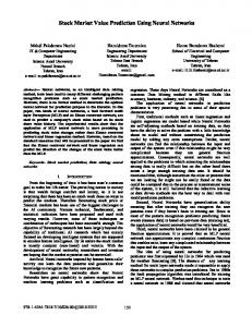
The space of possible intermarkets for the Australian stock market is not limited to these. However, these intermarkets (18)–(22) provide the most influential parts of the global economical system affecting the Australian stock market. Candidates of the additional input features selected from these intermarkets are the relative returns in the form of either (12) or (16). If the prediction horizon is just the next day, the relative returns of the intermarkets at the latest time t are sufficient; if the horizon is longer, then at least a short-term time series of the relative returns of one of the intermarkets should be used, together with the relative return time series of the target market such as (13) or (15). The data set for the target market and all the intermarkets used for this research corresponds to a period of about 13.5 years from January 1990 to August 2003. Figures 1–2 and Tables 1–2 show the autocorrelation and partial autocorrelation of the target market X = Australian All Ordinary Index (AORD) relative return as defined by (12). From the autocorrelation and partial autocorrelation tables (Tables 1–2), we can clearly see that there is a 6day cycle in the Australian stock market. These unusually large values are highlighted in the tables: 1-day lag, 6-day lag, 12-day lag, and 18-day lag. This is a surprise to us as we usually assume there is a 5-day cycle, known as the Day of the Week. Lag 1 2 3 4 5 6 7 8 9 10 11 12 13 14 15

ACC 0.05 -0.03 -0.00 -0.01 -0.01 -0.04 -0.03 0.02 0.01 -0.02 0.01 0.06 0.02 0.01 -0.01

Lag 16 17 18 19 20 21 22 23 24 25 26 27 28 29 30

ACC -0.01 0.02 -0.05 -0.02 0.01 0.01 -0.01 0.01 0.01 -0.01 0.02 -0.02 0.00 -0.01 0.00

Lag 31 32 33 34 35 36 37 38 39 40 41 42 43 44 45

ACC -0.02 -0.01 0.01 -0.00 -0.00 -0.03 -0.01 -0.01 -0.00 0.03 -0.01 -0.00 0.00 0.00 -0.02

Lag 46 47 48 49 50 51 52 53 54 55 56 57 58 59 60

ACC -0.01 0.03 0.02 0.03 -0.01 0.01 0.02 -0.00 -0.00 0.02 -0.00 -0.02 0.00 -0.02 -0.00

Table 1: Autocorrelation coefficients (ACC) of X (Significant autocorrelations are highlighted) Journal of Research and Practice in Information Technology, Vol. 37, No. 1, February 2005

47

Predicting Australian Stock Market Index Using Neural Networks

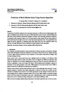
Figures 3 to 5 and Tables 3 to 5 show the cross correlation between X and each Yk, k = 1,2,3 as defined by (18)–(20). The correlation between X(t) and Y k (t–1), for k = 1,2,3, are extremely high, that between X(t) and Y k (t) are also very significant. Significant correlation between Y 1 (t) and

Figure 1: Autocorrelation function of X

Lag 1 2 3 4 5 6 7 8 9 10 11 12 13 14 15

PACC 0.05 -0.03 -0.00 -0.01 -0.01 -0.04 -0.02 0.02 0.01 -0.02 0.01 0.05 0.02 0.02 -0.00

Lag 16 17 18 19 20 21 22 23 24 25 26 27 28 29 30

PACC -0.01 0.02 -0.04 -0.01 0.01 0.01 -0.01 0.01 -0.02 0.01 -0.02 -0.01 0.00 -0.01 0.01

Lag 31 32 33 34 35 36 37 38 39 40 41 42 43 44 45

PACC -0.02 -0.01 0.01 -0.00 -0.00 -0.03 -0.01 -0.01 -0.00 -0.01 -0.01 -0.01 0.00 0.00 -0.02

Lag 46 47 48 49 50 51 52 53 54 55 56 57 58 59 60

PACC -0.01 0.03 0.02 0.03 -0.01 0.01 0.01 -0.00 0.00 0.02 -0.00 -0.02 0.01 -0.02 -0.01

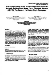
Table 2: Partial Autocorrelation coefficients (PACC) of X (Significant partial autocorrelation coefficients are highlighted) 48

Journal of Research and Practice in Information Technology, Vol. 37, No. 1, February 2005

Predicting Australian Stock Market Index Using Neural Networks

each of Y 4 (t),Y 5 (t) are also found as expected according to our empirical knowledge. Therefore, Y 4 (t),Y 5 (t) should also be included in the intermarkets of X(t). 5. PREDICTION OF THE NEXT-DAY MARKET DIRECTION With a series of daily returns as input vector, we expect to be able to predict the next-day market direction. According to the result of our statistical data mining (Figures 1 and 2), the Australian stock index, AORD, shows clearly cyclic behaviour with period 6 days. Therefore, we decided to use the last 6 daily returns of the close prices of AORD in the input vector. Among the inter-markets

Figure 2: Partial autocorrelation coefficients (PACC) of X

Lag 0 1 2 3 4 5 6 7 8 9 10

CCC 0.093 0.488 0.009 0.028 0.003 0.01 -0.011 -0.006 -0.031 0.027 -0.003

Lag 11 12 13 14 15 16 17 18 19 20 21

CCC -0.007 0.019 0.015 0.026 0 0.009 -0.001 -0.003 -0.039 -0.009 0.001

Table 3: Cross Correlation coefficients (CCC) between X and Y1 = S&P 500 Journal of Research and Practice in Information Technology, Vol. 37, No. 1, February 2005

49

Predicting Australian Stock Market Index Using Neural Networks

(18)–(22) considered, Y1- (US S&P 500 Index) shows the highest correlation to the target market. So its previous day’s relative return of the close price was also included in the input vector. In addition, the day of the week as a time signature was also included as an additional input in our experiments. The number of hidden layers are limited to 1or 2, and the number of hidden neurons for each hidden layer ranges from 2 to 50 in our experiments. The historical index time series data of DX(t) and DY(t) between January 1990 and August 2003 were used. The whole data set is divided into two data sets: 20% of the data are randomly selected and put into the test data set, and the remaining 80% into the training data set.

Figure 3: Cross correlation between X and Y1 = S&P 500

Lag 0 1 2 3 4 5 6 7 8 9 10

CCC 0.115 0.467 0 0.031 -0.001 0.009 -0.005 -0.005 -0.023 0.018 -0.007

Lag 11 12 13 14 15 16 17 18 19 20 21

CCC -0.009 0.01 0.011 0.017 -0.001 0.014 -0.003 -0.003 -0.043 -0.015 -0.001

Table 4: Cross Correlation coefficients (CCC) between X and Y2 = Dow Jones 50

Journal of Research and Practice in Information Technology, Vol. 37, No. 1, February 2005

Predicting Australian Stock Market Index Using Neural Networks

The performance of neural networks are measured in terms of root mean squared error (RMSE) and variance reduction (VR) for the training data set, and the sign correctness percentage (SCP) for testing the trained network on the test data set. Let N 1 ,N 2 be the number of data points for the training data and the test data respectively, then N 1 +N 2 = N is the total number of data points. The RMSE and VR for the training data are calculated as (23)

Figure 4: Cross correlation between X and Y2 = Dow Jones

Lag 0 1 2 3 4 5 6 7 8 9 10

CCC 0.099 0.398 0.022 -0.001 -0.006 0.009 -0.003 0.003 -0.023 0.039 0.009

Lag 11 12 13 14 15 16 17 18 19 20 21

CCC -0.022 0.022 0.022 0.027 0.005 0.009 -0.007 0.013 -0.031 0.006 -0.01

Table 5: Cross Correlation coefficients (CCC) between X and Y3 = NASDAQ Journal of Research and Practice in Information Technology, Vol. 37, No. 1, February 2005

51

Predicting Australian Stock Market Index Using Neural Networks

Figure 5: Cross correlation between X and Y3 = NASDAQ

(24)

where z k ,o k are the desired and actually calculated output for the k-th data point in the training data set, z– is the mean of {zk | k=1,2,…,N1}. The SCP for the testing data set is defined as (25)

where | {} | denotes the number of elements in the given set. 6. FINDING AN OPTIMAL ARCHITECTURE OF THE NEURAL NETWORK PREDICTOR Fixing the number of nonlinear hidden layers to one, we did a number of experiments using different random data samplings in order to discover the optimal number of hidden neurons. Table 6 shows experiment results of ten data sets randomly sampled from the original data set. For each data set, we let the number of hidden neurons run from 2 to 10, so in fact 9 neural networks were trained for each data set. The number of hidden neurons shown in the table for each sampled data set produced the best performance on the test data complimentary to that sampled training data. From these results, we take the mode of the 10 best numbers of hidden neurons, which is 2. Then with the number of hidden neurons fixed to 2, we further trained a number of neural networks, experimenting with various types of additional information. Table 7 shows the results of using different inputs for predicting X(t+1). 52

Journal of Research and Practice in Information Technology, Vol. 37, No. 1, February 2005

Predicting Australian Stock Market Index Using Neural Networks

Data Set 1 2 3 4 5 6 7 8 9 10

No. of Hidden Neurons 2 2 2 2 2 3 2 4 2 5

RMSE

SCP

0.5289 0.5274 0.5321 0.5204 0.5313 0.5357 0.5252 0.5400 0.5271 0.5363

80.26 77.27 77.27 78.12 80.26 77.27 78.84 79.12 76.85 78.84

Table 6: Cross validation for finding the optimal number of hidden neurons

Input Vector X(t– k), k=0,1,…5, only With (S&P 500) added With the Day of the Week added

RMSE 0.57 0.54 0.53

VR 50.80% 56.85% 57.26%

SCP 65% 76% 80%

Table 7: Training and testing results with different inputs

According to the SCP scores, the US S&P 500 index and the day of the week have added 11% and 4 % additional information to the prediction based on the Australian stock market index alone. However, it must be pointed out that prediction of different time frames requires different input selections, which may lead to significantly different network architectures. 7. FURTHER POSSIBILITIES So far we have only investigated very basic aspects of the problem. The results obtained are already very useful and the trained neural networks have been used routinely to generate daily predictions on the Australian stock index in our real-money stock and index futures trading. However, it should be pointed out that developing a specific neural network or a set of neural networks for this prediction purpose is a never-ending evolutionary process due to reflexivity (Soros, 2003) or everchanging cycles in financial markets. Further possibilities for improving the correctness, accuracy and reliability of the prediction include selection of technical indicators, in particular, those based on wavelet and fractal analysis, prediction of marginal probability distribution, ensembles or committees of neural networks, profit-driven genetic training algorithms, finer representation of time signatures such as using complex numbers for the day of the week, the day or week of the month, the day or week or month of the year in the input vector, and so on. 8. CONCLUSIONS In light of our empirical knowledge about the Australian stock markets and its interrelated international financial markets, we have investigated several aspects of input feature selection and the number of hidden neurons for a practical neural network for predicting Australian stock market index AORD. A basic neural network with limited optimality on these aspects has been developed, Journal of Research and Practice in Information Technology, Vol. 37, No. 1, February 2005

53

Predicting Australian Stock Market Index Using Neural Networks

which has achieved a correctness in directional prediction of 80%. This neural network takes the last 6 daily returns of the close price of the target market, the last daily return of US S&P 500 index, and the day of the week as the input features. Through a cross validation with a number of random data sampling, we found the optimal number of hidden neurons to be between 2 to 3. In additional to this development, a 6-day cycle has been discovered in the Australian stock market for the first time, of course subject to the historical time period studied. These results shed strong light on further research and development directions. In particular, we believe the probability ensemble of neural networks is one of the most promising directions. REFERENCES AZOFF, E.M. (1994): Neural Network Time Series Forecasting of Financial Markets. Wiley. BAESTAENS, D.E., VAN DEN BERG, W.M. and VAUDREY, H. (1995): Money market headline news flashes, effective news and the DEM/USD swap rate: An intraday analysis in operational time. Proc. 3rd Forecasting Financial Markets Conference, London. CYBENKO, G. (1988): Continuous valued neural networks with two hidden layers are sufficient. Technical report. Department of Computer Science, Tufts University, Medford, Massachusetts, USA. CYBENKO, G. (1989): Approximation by superpositions of a signoidal function. Mathematics of Controls, Signals and Systems 2:303–314. FISHMAN, M.B., BARR, D.S. and LOICK, W.J. (1991): Using neural nets in market analysis. Technical Analysis of Stocks and Commodities 9(4):18–22. GATELY, E. (1996): Neural Networks for Financial Forecasting. Wiley. HORNIK, K., SINCHCOMBE, M. and WHITE, H. (1989): Multilayer feedforward networks are universal approximators. Neural Networks 2:259–366. KATZ, J.O. (1992): Developing neural network forecasters for trading. Technical Analysis of Stocks and Commodities 10(4). KEAN, J. (1992): Using neural nets for intermarket analysis. Technical Analysis of Stocks and Commodities 10(11). MURPHY, J. (1999): Technical Analysis of the Financial Markets: A Comprehensive Guide to Trading Methods and Applications. Prentice Hall Press. PAN, H.P. (2003b): A joint review of technical and quantitative analysis of the financial markets towards a unified science of intelligent finance. Proc. 2003 Hawaii International Conference on Statistics and Related Fields, June 5–9, Hawaii, USA. PAN, H.P. (2003a): Swingtum – A computational theory of fractal dynamic swings and physical cycles of stock market in a quantum price-time space. Ibid. PAN, H.P. and FOERSTNER, W. (1992): An MDL-principled evolutionary mechanism to automatic architecturing of pattern recognition neural network. IEEE Proc. 11th International Conference on Pattern Recognition, the Hague. QI, M. (1999): Nonlinear predictability of stock returns using financial and economic variables. Journal of Business and Economic Statistics 17:419–429. REFENES, A. P., ABU-MOSTAFA, Y., and MOODY, J. (1996): Neural Networks in Financial Engineering. Proc. 3rd International Conference on Neural Networks in the Capital Markets. WEIGEND A. (eds). World Scientific. ROGERS, R. and VEMURI, V. (1994): Artificial Neural Networks Forecasting Time Series. IEEE Computer Society Press, Los Alamitos, CA. RUGGERIO, M. (1994): Training neural nets for intermarket analysis. Futures, Sep:56–58. SHIH, Y.L. (1991): Neural nets in technical analysis. Technical Analysis of Stocks and Commodities 9(2):62–68. SOROS, G. (2003): The Alchemy of Finance. Wiley, reprint edition. STEIN (1991): Neural networks: from the chalkboard to the trading room. Futures, May:26–30. SWALES, G.S. and YOON, Y. (1992): Applying artificial neural networks to investment analysis. Financial Analysts Journal 48(5). UTANS, J. and MOODY, J.E. (1991): Selecting neural network architectures via the prediction risk: application to corporate bond rating prediction. Proc. 1st Int. Conference on AI Applications on Wall Street, IEEE Computer Society Press. VIRILI, F. and REISLEBEN, B. (2000): Nonstationarity and data preprocessing for neural network predictions of an economic time series. Proc. Int. Joint Conference on Neural Networks 2000, Como, 5: 129–136. WARD, S. and SHERALD, M. (1995): The neural network financial wizards. Technical Analysis of Stocks and Commodities, Dec:50–55. WHITE, H. (1988): Economic predictions using neural networks: the case of IBM daily stock returns. Proc. IEEE International Conference on Neural Networks, 2: 451–458. WONG, F.S. (1992): Fuzzy neural systems for stock selection. Financial Analysts Journal, 48:47–52. YAO, J.T. and TAN, C.L. (2001): Guidelines for financial forecasting with neural networks. Proc. International Conference on Neural Information Processing, Shanghai, China, 757–761.

54

Journal of Research and Practice in Information Technology, Vol. 37, No. 1, February 2005

Predicting Australian Stock Market Index Using Neural Networks

BIOGRAPHICAL NOTES Dr Heping Pan has led the Intelligent Finance Cluster, CIAO, School of IT & MS, University of Ballarat since 2003. He is an internationally recognized expert on intelligent finance, information fusion and image analysis through a number of research and professorial positions in China, Europe and Australia. His current interests of research include super Bayesian influence networks – nonlinear dynamic Bayesian networks of probability ensembles of neural networks; intelligent finance theories and frameworks for integrating and unifying quantitative, technical and fundamental analysis of financial markets; and developing Global Influence Networks – a huge real-time, in-situ, complex system for modelling and prediction of world major financial markets.

Heping Pan

Chandima D. Tilakaratne is currently a PhD student at the Centre for Informatics and Applied Optimisation of the School of Information Technology and Mathematical Sciences, University of Ballarat, Australia. Her research interest includes the prediction of Stock Market Indices using neural networks. She is a lecturer attached to the University of Colombo, Sri Lanka, and received her BSc degree in 1990 and the MSc degree in 1996, from the same university. She is a member of the Association of Applied Statisticians, Sri Lanka. Chandima Tilakaratne

John Yearwood is Associate Professor of Information Technology at the University of Ballarat. He is leader of the Data Mining and Informatics Research Group in the Centre for Informatics and Applied Optimization. Dr Yearwood has published widely in the areas of Decision Support and Data Mining. His current research interests include narrative models, reasoning and argumentation, ontologies, artificial neural networks and data mining.

John Yearwood

Journal of Research and Practice in Information Technology, Vol. 37, No. 1, February 2005

55