Predicting Stock Market Price Using Support Vector ... - IEEE Xplore

Predicting Stock Market Price Using Support Vector Regression Phayung Meesad

Risul Islam Rasel

Faculty of Information Technology King Mongkut’s University of Technology North Bangkok Email: [email protected]

Dept of Computer Science & Engineering University of Chittagong, Bangladesh 4000 Email: [email protected]

Abstract— In this study, support vector regression (SVR) analysis is used as a machine learning technique in order to predict the stock market price as well as to predict stock market trend. Moreover, different types of windowing operators are used as data preprocess or input selection technique for SVR models. This is a new approach which uses different types of windowing functions as data preprocess for predicting time series data. Support vector regression is a useful and powerful machine learning technique to recognize pattern of time series dataset. It can produce good prediction result if the value of important parameters can be determined properly. Different kinds of Windowing operators are used in this experiment in order to feed more reliable inputs into regression models. This study is done on a well known company of Dhaka stock exchange (DSE), named ACI group of company Limited. Four year’s historical time series dataset are collected from the DSE from 2009 to 2012, as daily basis for experimentations. Finally, predicted results from WinSVR models are compared with actual price values of DSE to evaluate the model prediction performance.

SVM has two major applications, classification and regression [10]. One of the main characteristics of Support Vector Regression (SVR) is that instead of minimizing the observed training error, SVR attempts to minimize the generalized error bound so as to achieve generalized performance [11]. This generalization error bound is the combination of the training error and a regularization term that controls the complexity of the hypothesis space [12][13]. Kim [1], examined the feasibility of applying SVM in financial forecasting by comparing it with back-propagation neural networks and case-based reasoning. The experimental results showed that SVM provides a promising alternative to stock market prediction. Lai and Liu [3] showed in their research that SVM can be more accurate in producing result if we can chose the best combination of SVM parameters. They compared the prediction performances of NN and SVM in predicting exact stock prices on the Hang Seng Index (HSI) over 5 days and a 22 days horizon. The preprocessing or input selection techniques for SVR and NN used 15 days Exponential Moving Average (EMA15) and relative difference in percentage of price (RDP) RDP-5, RDP-10, RDP-15, and RDP-20. The best MAPE result was 0.8 for the year of 2008 short term forecast (5 days). For long term prediction (22 days), the best result was 4.33 also for the 2008 dataset. The average result was 5.02. Ince & Trafalis [2] showed the way how Kernel Principal Component can be analyzed to get better prediction results in his study. The motivation from those works are applied to the SVR as a machine learning technique using different windowing functions as data preprocess steps. This is a new approach to combine windowing operator and SVM together namely WinSVR model. This paper consists of five sections. Section II introduces the basic concept of SVR. Section III is about the experiment design. Section IV is about the experiment and result analysis. Section V is about the conclusions, limitation and future work of this study.

Keywords— Support vector regression (SVR); Windowing operators; Stock market; and Time series data.

I.

INTRODUCTION

The stock market is an emerging sector in any country of the world. Many people are directly related to this sector. So, it is important for those people to gain insight about the market trend. Along with development of the stock market, forecasting stock price has become an important topic among the people. Trend forecasting becomes an essential topic for stockholders, investors and the authority that are related to the stock market business. Predicting stock price is regarded as a challenging task [1]. Because stock markets are essentially a non-linear, nonparametric, noisy and deterministically chaotic system [2][3]. Trend of a market depends on many things like liquid money, stocks, human behavior, news related to stock market etc. All this together controls the behavior of trends in a stock market. The behavior of trend can be analyzed by using technical tools, parametric pricing methods or combination of these methods [4][5]. Many machine learning techniques have been used in recent time to predict the stock price. Neural network and support vector machine are the most usable among those [6][7]. SVM and NNs are both standard machine learning approaches to predict time series data [8][9].

II.

METHODOLOGY

In this study, the application of a new approach of combining support vector regression (SVR) and windowing function together is proposed. Windowing functions are used as data preprocess to select input for the machine learning technique in order to recognize the pattern of the dataset. Many machine learning techniques have been used in other recent researches [14]. In this study, the support vector regression

978-1-4799-0400-6/13/$31.00 ©2013 IEEE

(SVR) is used as a machine learning technique for pattern recognition. A. Support vector Regression (SVR) SVM regression perform linear regression in the high dimension feature space using f - insensitivity loss and, at the same time tries to reduce model complexity by minimizing | | w | | 2 . This can be described by introducing slack variables * p i and pi where i = 1, ..., n to measure the deviation of

* y i - f(x i, w) # f + pi Min * f(x i, w) - y i # f + p i * p i, pi $ 0, i = 1, ...., n

Actual close price of ACI com pany 600

(1)

(2)

500 Price (BDT)

training sample outside f - sensitive zone [3][9][13]. n 1 * U (w, p) = 2 | | w | | + C / _p i + pi i i=1

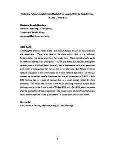
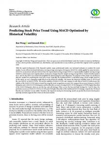
and volumes. But from this dataset only 5 attributes are used for the experiments. Date as ID, open price, high price, low price and close price are as regular attributes. The goal is to predict close price for some specific amount of time a-head, such as 1 day a-head, 5 days a-head, and 22 days a-head. We separate dataset into 2 groups. Training dataset (80%) and testing dataset (20%). 2009-2011 data are used as a training dataset and 2012 data are used as a testing dataset. Fig.1 shows the actual close price for ACI group of Company Bangladesh for the year of 2009 to 2012.

200

0 1

54 107 160 213 266 319 372 425 478 531 584 637 690 743 796 Days (Jan'09-Jun'12) Actual close price

Fig. 1. Data set sample

* Subject to, 0 # ai # C, 0 # a i # C where n sv is the number of support vector (SVs) and the kernel function m K(x, xi) = / j = 1 g(x)g j (xi) (4)

SVM generalization performance depends on a good setting of kernel parameters C, f and kernel parameters [9][13]. To evaluate the result from the SVR models, Eq. (5) is used to measure the error rate.

(5)

Here MAPE stands for Mean average percentage error between actual share prices (A) and predicted share price (P). And ‘n’ is the number of days to take into count. III.

300

100

This optimization problem can transform into the dual problem and solution is given by nsv f(x) = / (a i - ai*)K(x i, x) (3) i=1

n /i 1 | A - P | = A MAPE = 100 n

400

B. Model Setting and Analysis steps The experimentation models are started with data preprocesses steps to produce inputs for SVR. For that, different kinds of windowing operators, such as basic rectangular windowing, flatten windowing and de-flatten windowing were used as input selection techniques. Windowing operator transforms the time series data into a generic data set to input this data into the learning algorithm. In this study, the support vector regression (SVR) is used as a learning algorithm to learn pattern from the input and to predict stock price as output based on that learning. This study is conducted in two phases, training phase and testing phase. Steps from these two phases are given below: 1) Training phase • Step 1: Read the training dataset from local repository. •

Step 2: Apply windowing operator to transform the time series data into a generic dataset. This step will convert the last row of a window within the time series into a label or target variable. Last variable is treated as label.

•

Step 3: Accomplish a cross validation process of the produced label from windowing operator in order to feed them as inputs into SVR model.

•

Step 4: Select kernel types and select special parameters of SVR (C, f , g etc).

•

Step 5: Run the model and observe the performance (accuracy).

EXPARIMENT DESIGN

A. Research Data In order to undertake the experiments and evaluate the results from the experiments, Dhaka stock Exchange (DSE), Bangladesh was selected as our research domain. For that, the collection of 4 years (2009-2012) historical time series dataset from DSE was gathered. Primarily, the collection of all stock price information for all the listed company of DSE was gathered. But for the convenience of research purpose, only one well known listed company from DSE was selected to do experimentations. The name of this company is ACI group of company Limited, Bangladesh. The original dataset contains 6 attributes. Date, open price, high price, low price, close price

•

Step 6: If performance accuracy is good than go to step 6, otherwise go to step 4.

•

Step 7: Exit from the training phase & apply trained model to the testing dataset.

selecting appropriate kernel function and its parameters setting. Here, RBF kernel function is used because it is faster and also able to produce good output result. Table 2 shows the kernel components value that helps to produce good prediction result from this analysis.

2) Testing phase • Step 1: Read the testing dataset from local repository. •

Step 2: Apply the training model to test the out of sample dataset for price prediction. Step 3: Produce the predicted trends and stock price

•

IV.

EXPARIMENTS & RESULTS

A. Data preprocess (windowing operator) The 1st step of this experiment is to preprocess the data set for selecting input for the SVR models. To do so, three different kinds of windowing operators were used to produce generic data from time series data. After completing iterative analysis, it was found that a good combination of windowing components values were able to produce good inputs for the support vector regression (SVR) models. Table 1 shows the window settings that produce inputs for the support vector regression analysis. TABLE I. Windowing operator Rectangular Flatten window De-Flatten window

Model All 1 day 5 days 22 days All

WINDOW SETTINGS

Window size

Step size

3 3 8 25

1 1 1 1

5

Training window width 30 30 30 30

1

Test window width 30 30 30 30

30

B. SVR kernel function analysis After input selection process, the next step is to apply the learning technique. In this study, the support vector regression (SVR) is used as learning technique. It is commonly known that the proper output from SVR model mostly depends on

Model 1 day

SV 696

3.335

687

-4.658

653

-14.893

C

Kernel

g

ε

ε+

ε-

RBF

10000

1

2

1

1

Model-2

RBF

10000

1

2

1

1

Model-3

RBF

10000

1

2

1

1

C. SVR Models To undertake the experiments, three separate models were created for predicting stock price over 1 day a-head, 5days ahead, & 22 days a-head. Model-1 is for 1 day a-head, Model-2 is for 5 days a-head & Model-3 is for 22 days a-head prediction. Table III, IV & V show the respective model description in tabular format. And table VI shows the prediction results come from different Win-SVR models. The result table contains the actual and predicted share price of ACI group of Company Bangladesh, for the month of January 2012 to May 2012. The average error between the actual and predicted price (MAPE) are given in table VII. TABLE III.

SVR MODEL FOR NORMAL RECTENGULAR WINDOW

Support Vector

Bias (offset)

SV

b

w [close-2]

Weight (w) w [close1]

w [close0]

1 day

696

400.7

1358.9

627.1

501.1

5 days 22 days

692

381.5

825.1

734.1

-297.1

675

421.3

1719.6

1631.5

805.1

In table III & V, the weight (w) comes from only close attributes because only a single attribute was selected to analyze the models. Single attribute weights produce good results over the multiple attributes in those models.

SVR MODEL FOR FLATTEN WINDOW

Bias (b)

5 days

22 days

SVR Model

KERNEL PARAMETER SETTINGS

Model-1

Model

30

TABLE IV.

TABLE II.

w[open-2] -746.516 w[open-7] 1792.63 w[Low-7] 2587.202 w[open-24] 2481.053 w[Low-24] 3564.178

Table IV shows the models are selected from the flatten window. Here, all major attributes were selected because it creates good results over using a single attribute. So, weights

w[High-2] -1074.989 w[open-6] 1716.616 w[Low-6] 2219.727 w[open-23] 2109.68 w[Low-23] 3218.868

Weight (w) w[Low-2] -1087.763 w[High-7] 2231.12 w[Close-7] 2762.02 w[High-24] 3379.996 w[Close-24] 3962.164

w[Close-2] -546.558 w[High-6] 2447.79 w[Close-6] 2187.662 w[High-23] 3094.46 w[Close-23] 3204.893

(w) comes from all major attributes like open, high, low and close. Offset value (bias) and number of support vector (SV) are also given for specific models. Table V shows the model

description which comes from de-flatten window, also using only a single attribute like the rectangular window models. TABLE V. Model 1 day 5 days 22 days

SV 694

SVR MODEL FOR DE-FLATTEN WINDOW

Bias (b)

Weight (w)

877.156

690

874.17

673

762.739

w[Close-4]

w[Close-3]

w[Close-2]

w[Close-1]

3513.379

3918.574

5301.521

4699.025

w[Close-4]

w[Close-3]

w[Close-2]

w[Close-1] 5639.484

2890.699

2450.3

4085.636

w[Close-4]

w[Close-3]

w[Close-2]

w[Close-1]

745.48

-1181.587

-1091.834

-2042.671

Table VI shows the experiment results from different WinSVR models. This table contains actual close price of ACI group which was collected from the DSE database. Stock Prices from January 2012 to May 2012 were the testing dataset for this study. So, the actual share price and predicted share price of ACI group of company are tabulated in this table for this timestamp only. The difference between actual and predicted price (error) is given below in table VII. From table VI and VII, it is easy to understand that flatten window can produce good prediction result using the support vector regression technique. And Normal rectangular window also can TABLE VI. Window Name Rectangular

Flatten window

De- Flatten

Month

Only the close prices values are used to built and analyze the models.

produce good results too. But, the results come from de-flatten window are the worst among these three types of windowing operators. The best result from this study comes from flatten window for 1 day a-head prediction. The error rate was 0.04. It means that the predicted prices were very close to the actual prices. The next best result for 5 days a-head prediction comes from flatten window also and the error rate was 0.15. The 3rd and final best result for 22 days a-head prediction comes from rectangular window and flatten window both. The error rate was 0.22.

RESULT TABLE FOR ALL WIN-SVR MODELS

Actual price (BDT)

Predicted price (BDT) 1 day a-head

5 days a-head

22 days a-head

Jan'12

4016.5

4147.85

4156.26

3876.92

Feb'12

3341.4

4241.33

3783.34

3138.04

Mar'12

4032.8

4110.07

4062.15

3906.77

Apr'12

5300.1

5218.71

5220.05

4979.68

May'12

4280.3

4578.76

4558.99

3825.77

Jan'12

4016.5

4057.3

3112.3

N/A*

Feb'12

3341.4

3319.6

3319.7

2937.2

Mar'12

4032.8

4009

3899.6

3899.6

Apr'12

5300.1

5269.5

5139.4

5139.4

May'12

4280.3

4349.2

4601

4224.7

Jan'12

3583.3

8049.41

7312.12

7816.93

Feb'12

3341.4

12758.09

12914.58

12792.77

Mar'12

4032.8

9201.99

8188.38

9229.55

Apr'12

5300.1

10268.98

9561.42

9414.87

May'12

4280.3

10127.33

9556.45

8595.15

N/A* Flatten window 1st removed all attributes lying between the time point zero (attribute name ending "-0") and the time point before horizon values. Second, it transforms the corresponding time point zero of the specified label stem to the actual label. Last, it re-represents all values relative to the last known time value for each original dimension including the label value. so, it produces result exactly after from horizon selected.

D. Error calculation (MAPE) SVR models produce the prediction result based on the model design. The error rate is computed between the actual stock prices and predicted stock price come from the experiments. To calculate the error rate, Mean average percentage error (MAPE) is used in this study. The MAPE equation is described in introduction section of this paper (eq.5). Table VII shows the error (average MAPE) committed

in different SVR models using different kinds of windowing operators. The calculation of MAPE was only done for the testing dataset. MAPE results were calculated as monthly basis for the month of January 2012 to May 2012. From the table VII, it is easy to understand that models are created by using normal rectangular window and flatten window can produce good prediction results. Because prediction prices from these

two are very close to the actual prices. So, error rate is very low. But de-flatten window can not produce good prediction result because of high prediction error rate.

Actual vs Predicted close price 22 days a-head m odel

MAPE (ERROR) FOR TEST DATA (FROM JAN’12 TO MAY’12)

Model

Rectangular window 0.42 0.26 0.22

Horizon

1 Day a-head 5 days a-head 22 days a-head

1 5 22

Flatten window 0.04 0.15 0.22

De-flatten window 7.79 7.16 7.61

E. Graphical analysis In this study, nine different SVR models were created by using three different types of windowing operators. Some of them are good enough to produce good prediction results but some are not. Such as, the models which were created from de-flatten windowing operator were not good enough to produce good prediction results. Because the predicted result produced from those model are so erroneous. But models which are created from rectangular and flatten window were good enough to predict price. Figure 2 shows the model result for 1 day a-head prediction. This model is built by using flatten windowing operator. Average MAPE of this model is 0.04.

300 Close Price (BDT)

TABLE VII.

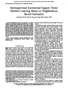
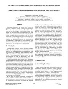
Figure 4 shows the results from the SVR model using rectangular window for 22 days a-head stock price prediction. The average MAPE (error) of this model is 0.22.

200 150 100 50 0 1

6 11 16 21 26 31 36 41 46 51 56 61 66 71 76 81 86 91 96 Days (Jan-May'2012) Actual

Predicted

Fig. 4. Output from Win-SVR model using rectengular window (22days)

Figure 5 shows the error rate from the SVR models which are built by using rectangular windowing operator. Error rate Norm al Rectangular w indow 1.5

MAPE

Actual vs Predicted price 1 day a-head model

Close Price (BDT)

250

300 250 200 150 100 50 0

1 0.5 0 Jan

Feb

Mar

Apr

May

Month 1

10

19

28

37

46

55

64

73

82

91 100 109 118

1 day a-head

5 days a-head

22 days a-head

Days (Jan-Jun'2012) Predicted

Fig. 2. Output from Win-SVR model using flatten window (1day)

Figure 3 shows the graphical representations of the results from the SVR model using flatten window for 5 days a-head stock price prediction. The average MAPE (error) of this model is 0.15. Actual vs Predicted price 5 days a-head model

Close price (BDT)

300

Fig. 5. MAPE for rectangle window models

Figure 6 shows the error rate from the SVR models which are built by using flatten windowing operator. Error rate Flatten w indow 0.50 0.40 MAPE

Actual

0.30 0.20 0.10 0.00

250 200

Jan

Feb

Mar

Apr

May

150

Month

100 50

1 day a-head

0 1

6

11 16 21 2 31 3

41 4

51 56 61 6

5 days a-head

22 days a-head

71 76 81 8 91 9 10 10 111

Days (Jan-jun'2012)

Fig. 6. MAPE for flatten window models Actual

Predicted

Fig. 3. Output from Win-SVR model using flatten window (5days)

Figure 7 shows the error rate from the SVR models which are built by using de-flatten windowing operator.

ACKNOWLEDGMENT

MAPE

Error rate De-flatten w indow

Authors are very grateful to Mr. Ashraf Uddin, Sr. Executive at Lanka Bangla Securities Ltd, for providing us the stock index data from Dhaka stock exchange (DSE), Bangladesh.

16 14 12 10 8 6 4 2 0

REFERENCES [1] Jan

Feb

Mar

Apr

May

[2]

Months 1 day a-head

5 days a-head

22 days a-head

Fig. 7. MAPE for de-flatten window models

From figure 5, 6, & 7 it is clear that the SVR models created by using de-flatten windowing operator are worse to predict good stock price. Because models are built from de-flatten window predict more erroneous price value. But models created by using rectangular and flatten window operator are good enough to produce good prediction results. V.

CONCLUSION

A. Discussion The motivation was to propose a model which will be able to produce good stock price prediction results. This study is done by combining different kinds of windowing function with a support vector machine. This is a new way to apply different kinds of windowing function as data preprocess step to feed the input into the machine learning algorithm for pattern recognition. From the result analysis, one can say that, SVR models that are built by using rectangular window and flatten window operator are good to predict stock price for 1 day ahead, 5 days a-head and 22 days a-head. Because Error rate (MAPE) between actual and predicted price values in those models is quite acceptable because of low margin difference. B. Limitation & futurework Three types of windowing operators were used in this study and only one dataset from the DSE Bangladesh was applied to train and test the models. In the future, some other windowing functions will be applied as input selection technique in order to improve the prediction performance of our proposed WinSVR model’s and the results will be compared with other data mining techniques by applying different dataset from different stock index.

[3]

[4]

[5]

[6]

[7]

[8]

[9]

[10]

[11]

[12] [13] [14]

Kim, Kyoung-jae, “Financial time series forecasting using support vector machines,” In: Neurocomputing 55, pp.307 – 319, 2003. H. Ince, T.B. Trafalis, “Kernel Principal Component Analysis and Support Vector Machines for Stock Price Prediction,” In: 0-7803-83591/04/ 2004 IEEE, pp. 2053-2058, 2004 Lucas, K. C. Lai, James, N. K. Liu, “Stock Forecasting Using Support Vector Machine,” In: Proceedings of the Ninth International Conference on Machine Learning and Cybernetics, pp. 1607-1614, 2010 Lu, Chi-Jie, Chang, Chih-Hsiang, Chen, Chien-Yu, Chiu, Chih-Chou, Lee, Tian-Shyug, “Stock Index Prediction: A Comparison of MARS, BPN and SVR in an Emerging Market,” In: Proceedings of the IEEE IEEM, pp. 2343-2347, 2009 K. S. Kannan, P. S. Sekar, M. M. Sathik, P. Arumugam, “Financial Stock Market Forecast using Data Mining Techniques,” In: Proceedings of the International Multiconference of Engineers and computer scientists, pp. 555-559, 2010 Yanjie. Hu, Juanjuan. Pang, “Financial crisis early warning based on support vector machine,” In: International Joint Conference on Neural Networks, pp. 2435-2440, 2008 Kuan-Yu. Chen, Chia-Hui. Ho, “An Improved Support Vector Regression Modeling for Taiwan Stock Exchange Market Weighted Index Forecasting,” In: The IEEE International Conference on Neural Networks and Brain, pp. 1633-1638, 2005 S. Xue-shen, Q. Zhong-ying, Yu. Da-ren, Qing-hua, Hu. Hui, Zhao, “A Novel Feature Selection Approach Using Classification Complexity for SVM of Stock Market Trend Prediction,” In: 14th International Conference on Management Science & Engineering, pp. 1654-1659, 2007 B. Debasish, P. Srimanta, C.P. Dipak, “Support Vector Regression,” In: Neural Information Processing – Letters and Reviews Vol. 11, No. 10, pp. 203-224, 2007 Chih-Wei. Hsu, Chih-Chung. Chang, Chih-Jen. Lin, “A Practical Guide to Support Vector Classification,” Initial version: 2003, Last updated version: 2010 U. Thissena, R. van. Brakela, A.P. de. Weijerb, W.J. Melssena, L.M.C. Buydensa, “Using support vector machines for time series prediction,” In: Chemometrics and Intelligent Laboratory Systems 69, pp.35– 49, 2003 Lijuan. Cao, “Support vector machines experts for time series forecasting,” In: Neurocomputing 51, pp. 321 – 339, 2003 J. Smola. Alex, SchoLkop. Bernhard, “A tutorial on support vector regression,” In: Statistics and Computing 14, pp.199–222, 2004 Ahmad Kazema, Ebrahim Sharifia, Farookh Khadeer Hussainb, Morteza Saberic,Omar Khadeer Hussaind, “support vector regression with chaos-based firefly algorithm for stock market price frocasting ,” In: Applied Soft Computing 13 , pp. 947–958, 2013