Predicting football scores via Poisson regression ... - ScienceCentral

Communications for Statistical Applications and Methods 2016, Vol. 23, No. 4, 297–319

http://dx.doi.org/10.5351/CSAM.2016.23.4.297 Print ISSN 2287-7843 / Online ISSN 2383-4757

Predicting football scores via Poisson regression model: applications to the National Football League Erlandson F. Saraivaa , Adriano K. Suzuki 1,b , Ciro A. O. Filho b , Francisco Louzada b a

b

Institute of Mathematics, Federal University of Mato Grosso do Sul, Brazil; ˜ Paulo, Brazil Department of Applied Mathematics and Statistics, University of Sao

Abstract Football match predictions are of great interest to fans and sports press. In the last few years it has been the focus of several studies. In this paper, we propose the Poisson regression model in order to football match outcomes. We applied the proposed methodology to two national competitions: the 2012–2013 English Premier League and the 2015 Brazilian Football League. The number of goals scored by each team in a match is assumed to follow Poisson distribution, whose average reflects the strength of the attack, defense and the home team advantage. Inferences about all unknown quantities involved are made using a Bayesian approach. We calculate the probabilities of win, draw and loss for each match using a simulation procedure. Besides, also using simulation, the probability of a team qualifying for continental tournaments, being crowned champion or relegated to the second division is obtained.

Keywords: prediction, football, attack and defense effect, Poisson regression, Bayesian inference, MCMC, simulation, de Finetti measure

1. Introduction Football, originally practiced in England, is one of the most popular collective sports worldwide. A particular characteristic of this sport is that the best team it is not always the winner of a match or a tournament, which causes a climate of expectation among players and fans. In the last few years, some studies have addressed the prediction of outcomes for matches of the World Cup, such as, Dyte and Clarke (2000), Volf (2009), and Suzuki et al. (2010). Dyte and Clarke (2000) proposed a Poisson regression model considering control variables, which consist of the rating for each team and the match venue given by the Federation Internationale of Football Association (FIFA). The authors used their results and other results about the quality of forecasts to simulate the 1998 FIFA World Cup. Volf (2009) consider a counting processes approach, in order to model a match score as two interacting time-dependent random point process. The interaction between teams are modeled via a semi-parametric multiplicative regression model of intensity. The authors applied this model to the analysis of the performance of the eight teams that reached the quarter-finals of the 2006 FIFA World Cup. Suzuki et al. (2010), proposed a Bayesian approach to predict of the outcomes of matches using specialists’ opinions and FIFA rankings to build a Power prior. Using simulations, the authors calculate the probabilities of wins, draws, losses and odds of the teams being ranked in the group stage 1

Corresponding author: Department of Applied Mathematics and Statistics, University of São Paulo, Avenida Trabalhador São-carlense, 400 - Centro CEP: 13566-59, São Carlos-SP, Brazil. E-mail: [email protected]

Published 31 July 2016 / journal homepage: http://csam.or.kr c 2016 The Korean Statistical Society, and Korean International Statistical Society. All rights reserved. ⃝

298

Erlandson F. Saraiva, Adriano K. Suzuki, Ciro A. O. Filho, Francisco Louzada

are obtained. Bastos and da Rosa (2013) developed a Bayesian methodology for the Poisson-gamma model in which the priors are chosen considering historical and recent information. The authors calculate the probabilities of win, draw and loss for the 2010 FIFA World Cup games. Several articles also focused on the prediction of outcomes in national leagues. Among them, Keller (1994) considered the Poisson distribution for the number of goals scored by England, Ireland, Scotland and Wales in the British International Championship (1883–1980). Lee (1997) developed a generalized linear model with application to final rank analysis. Brillinger (2008) modeled the probabilities of win, tie and loss through an ordinal-value model and applied the model to the Brazilian Series A championship. Karlis and Ntzoufras (2009) applied the Skellam’s distribution to model the difference of goals between home and away teams. The authors illustrated the model using the 2006– 2007 English Premier League. Koopman and Lit (2015) developed a statistical model to predict the games of the 2010–2011 and 2011–2012 English Premier Leagues, assuming a bivariate Poisson distribution with coefficients that stochastically changed intensity over time. An issue about papers cited above is that none consider the home team factor to calculate the probabilities of interest. For Maher (1982) it is important to add a constant factor to all teams when they play at home. Following this approach, Dixon and Coles (1997) presented a study considering 6,000 matches of English teams in the 1993–1995 period. Results showed that 46% of the matches was won by the home team, 27% were draws and in 27% the home team lost. In a similar study, KnorrHeld (2000) provided data of the 1996–1997 season of the German Bundesliga. Results showed that in 51% of the matches the win was of the home team and in only 26% the home team lost. Considering the season 2011–2012 of the English Premier League, 47% of the matches ended with win of the home team and only 27% ended with defeat of the home team. These results show us that, for some reason, there seems to be an inherent advantage for the team if it is playing at home. In this way, the effect of playing at home can be introduced in the model in order to predict the probabilities of win, draw and lose. In this paper, we model the number of goal scored by each team in a match by a Poisson distribution, whose average reflects the strength of the attack and defense of the team and effect of being playing at home. Inferences about all the unknowns quantities involved are made using a Bayesian approach. We illustrate the performance of the proposed method considering the outcomes of the 2012–2013 season of the English Premier League (EPL) and the outcomes of the 2015 Brazilian Football League (BFL). Using a simulation study, we calculate the probabilities of win, draw and lose for each team in each round of the EPL and BFL. We also present the probability of a team qualifying for the continental tournaments, being crowned champion or relegated to the second division. All computer implementations were performed using OpenBUGS (Spiegelhalter et al., 2003) and R systems (R Development Core Team, 2012) in the R2WinBUGS package (Gelman et al., 2006). The remainder of the paper is organized as follows. In Section 2, we present the Poisson regression model and expressions used to calculate the probabilities of win, draw and defeat for a football game. Sections 3 and 4 report results obtained by applying the proposed model for matches of the EPL and BFL, respectively. Section 5 concludes with some general remarks.

2. Model Consider a football championship with n + 1 teams, in which, each team plays 2n times, being n times at home stadium and n times at away stadium. The number of games of the championship is N = n(n + 1). The N games are played in two phases, each phase with N/2 games. If in the first

Predicting football scores via Poisson regression model

299

phase, a game between teams t and s occurs at home stadium of t team, then in the phase two the game occurs at home stadium of s team. By each result, victory, draw and defeat each team gets 3, 1 and 0 points, respectively. After the N games, the team with the highest score is declared champion. The M teams with smallest scores are relegated to the second division. In the EPL, M = 3, and in BFL, M = 4. For a game j between teams t and s, let Xt j and X s j be random variables denoting the number of goals of the home team and away team, respectively, for j = 1, . . . , n. Assume that, Xt j ∼ Poisson(λt j )

and

X s j ∼ Poisson(λ s j ).

(2.1)

In order to link the number expected of goals of teams t and s with their strength of attack (a), strength of defense (d) of the opposing team and the effect of being playing at home (h), we consider λk j = eUk j βk ,

(2.2)

for j = 1, . . . , 2n, where k = t, s, Uk j = (1, 1, 1, 1) if the game is at home stadium of k team and Uk j = (1, 1, 1, 0) otherwise, and βk = (βk0 , βka , βkc d , βkh )′ is the vector of parameters of the k team, where kc represents the opposing team. For example, if k = t, then kc = s. The parameter βka measures the attack strength of the k team and parameter βkc d measures the defense strength of the opposing team kc . The parameter βkh gives the advantage of playing at home, which we assume as being equals for every team of the championship. Note that, in this formulation a team with a good defense will have a negative defense effect because this will decrease the expected number of goals of the opposing team. In the other hand, a team with positive defense effect increases the expected number of goals of the opponent. Suppose that a game j is played in (r + 1)th round of the championship, 1 ≤ r ≤ N. Let nr be the number of games played by teams t and s before of the (r + 1)th round. Consider xk = (xk1 , . . . , xknr ) be the number of goals scored by k team in the nr games, in which, xkm is number of goals scored by the k team in the mth game, for k = t, s and m = 1, . . . , nr . Thus, the log-likelihood function for (βt , β s ) is given by l(βt , β s ; xt , x s ) =

nr ( ∑ ∑ ) −eUkm βk + xkm Ukm βk − log(xkm !) .

(2.3)

k∈{t,s} m=1

Some constraints must be imposed on team-specific parameters to avoid nonidentifiability. Following Karlis and Ntzoufras (2003) and Baio and Blangiardo (2010), we use a sum-to-zero constraint, i.e., n+1 ∑ t=1

βta = 0,

n+1 ∑ t=1

βtd = 0,

and

n+1 ∑

βth = 0,

(2.4)

t=1

i.e., the sum of the strength of the attack, defense and home effect of all (n + 1) teams is equal to zero. In order to develop the Bayesian approach we need to specify the prior distributions for parameters βk , k = t, s. We assume that priors are a priori independent, i.e., π(βt , β s ) = π(βt )π(β s ), in which, π(βk ) = π(βk0 )π(βka )π(βkd )π(βkh ), for k = t, s. So, we consider the following prior distributions: βk0 ∼ N(0, 10−4 ), βka ∼ N(0, 10−3 ), βkc d ∼ N(0, 10−3 ) and βkh ∼ N(0, 10−3 ), for k = t, s, where N(0, b) denotes the normal distribution with mean 0 and precision b. Joint posterior distributions for parameters do not have closed form; therefore, we estimate parameters βt and β s using MCMC. In Appendix A of the Supplementary Material (SM) we provide some


300

details of the estimation procedure using MCMC. All computer implementations were performed using OpenBUGS and R systems in the R2WinBUGS package. Estimates β˜ t and β˜ s are given by the average of the generated MCMC sample. Given β˜ t and β˜ s , we use these values to calculate the probability of a win, draw and defeat of each team in the next round.

2.1. Predictions Consider that a game j between teams t and s will occurs at home stadium of team t in (r + 1)th round of the championship. Denote the probability of win, draw and defeat (loss) of team t by Pw , Pd and Pl , respectively. These probabilities are given by g−1 ∞ ∑ ) ∑ ( ) ( ) ˜ ˜ Pw = P Xt j > X s j |βt , β s = P Xt j = g|β˜ t P X s j = u|β˜ s ,

(

(2.5)

g=1 u=0 ∞ ( ) ∑ ( ) ( ) Pd = P Xt j = X s j |β˜ t , β˜ s = P Xt j = g|β˜ t P X s j = g|β˜ s ,

(2.6)

g=0 ∞ ∑ u−1 ( ) ∑ ( ) ( ) Pl = P Xt j < X s j |β˜ t , β˜ s = P Xt j = g|β˜ t P X s j = u|β˜ s .

(2.7)

u=1 g=0

Similarly to Bastos and da Rosa (2013) and Suzuki et al. (2010) we calculate the de Finetti distance in order to measure the goodness of a prediction. This distance is given by the Euclidean distance between the point corresponding to the real outcome and the corresponding to the prediction. For this, is assumed that the set of all possible forecasts is given by the simplex set S = {(Pw , Pd , Pl ) ∈ R3 : Pw + Pd + Pl = 1, Pw ≥ 0, Pd ≥ 0, Pl ≥ 0} and that the possible real outcome, win, draw and defeat are represented by the points (1, 0, 0), (0, 1, 0) and (0, 0, 1), respectively. The de Finetti measure (df) is defined as: df = (Pw − b1 )2 + (Pd − b2 )2 + (Pl − b3 )2 , where (b1 , b2 , b3 ) ∈ {(1, 0, 0), (0, 1, 0), (0, 0, 1)}. For example, if the prediction for the game between teams t and s is (0.2, 0.65, 0.15) and the real outcome is (0, 1, 0), i.e., a draw, then the de Finetti distance is d f = (0.2 − 0)2 + (0.65 − 1)2 + (0.15 − 0)2 = 0.185. For the equiprobable case, Pw = Pd = Pl = 1/3, with win of the home team, (1, 0, 0), the de Finetti measure is given by d f = (1/3 − 1)2 + (1/3 − 0)2 + (1/3 − 0)2 = 2/3. This value is accepted as a threshold value in order to classify the predictions as acceptable or not, see for example Suzuki et al. (2010). If d f < 2/3, the predictions are considered acceptable; otherwise, d f > 2/3, the predictions are considered poor. Using a simulation procedure, we also calculate the probability of each team to be the champion. In order to calculate these probabilities we assume that the first phase of the champion is ended, i.e., n(n + 1)/2 games were played. Let T t be the number of points of the team t until the last game of the first phase. The simulation procedure is given by the following steps: (i) For the jth game of the second phase of the championship, j = (n(n + 1)/2) + 1, . . . , N, do as follows: (a) Get the estimates (β˜ t , β˜ s ) from Bayesian approach, where t and s represent the teams t and s;


301

(b) Given β˜ k , generate the number of goals scored by k team, Xk j , from a Poisson distribution ˜ with parameter λk j = eUk j βk , for k = t, s; (c) If Xt j > X s j , do T t = T t + 3 and T s = T s ; if Xt j = X s j , do T t = nT + 1 and T s = T s + 1; if Xt j < X s j , do T t = T t and T s = T s + 3; (d) Ended the second phase, the A team is declared champion if T A = max1≤t≤n T t . (ii) Repeat the step (i), r times, for r = 1, . . . , R. We consider R = 1,000. The probability of the team A be the champion is estimated by the proportion of times that A team is declared champion among the R simulated cases, i.e., NAchamp Pchamp (A) = , R where NAchamp is the number of times that team A is the champion among the R simulated cases. Similarly, the probability of team A be relegated to the second division is given by Preleg (A) =

NAreleg , R

where NAreleg is the number of times that team A finished as one of the M teams with smaller number of points among the R simulated cases. For EPL, M = 3, and for BFL, M = 4.

3. Application 1 In this section, we apply the proposed method to the 2012–2013 season of the EPL. EPL is composite by n + 1 = 20 teams. The number of games of the EPL is 380, being 190 by phase. Table 1 shows the number of games and the number of goals scored by each team at home and away in each phase of the EPL. Table 1 is ordered according to team with highest to smallest number of goals scored (last column). Manchester United has the highest number of goals scored, 86, being 45 scored at home and 41 away. Manchester United is also the team that has the highest number of goals scored away. In its home stadium, Manchester United, only scored less goals than Arsenal. Queens Park Rangers has the smallest number of goals scored, 30. This team, also has the smallest number of goals scored at home. West Ham United has the smallest number of goals scored at away. Table 2, shows the number of games ended with number of goals (xt , x s ), where xt and x s are the number of goals scored by home and away team, respectively. The sum of numbers of each column of this Table 2, give the number of games in which the home team scored xt goals. For instance, the sum of the second column is 120; meaning, that in 120 games the home team scored 1 goal. Analogously, the sum of numbers of each line of Table 2, give the number of games in which the away team scored x s goals. For instance, the sum of the fifth row is 15; meaning, that in 15 games the away team scored four or more goals. The main diagonal give the amount of ties. The total of ties is 109 (28.68%). The upper and lower diagonal give the number of games with win of the home and away team, respectively. Adding values of upper diagonal, we get the number of games won by home team, 166 (43.68%); while the sum of the values of the lower diagonal give the number of games won by the away team, 105 (27.64%).


302

Table 1: Number of games and goals scored by each team at home and away in each phase of the EPL 1st phase Games Games Goals Goals at home away Manchester United 09 26 10 22 Chelsea 10 24 09 15 Arsenal 09 23 10 14 Liverpool 10 14 09 14 Manchester City 10 22 09 12 Tottenham Hotspur 10 14 09 20 Everton 09 16 10 16 West Bromwich Albion 10 16 09 12 Fulham 09 16 10 13 Southampton 10 14 09 11 Aston Villa 09 08 10 07 Swansea City 10 17 09 10 Wigan 10 14 09 06 Newcastle United 10 12 09 11 West Ham United 10 17 09 06 Reading 09 14 10 07 Norwich City 09 10 10 10 Sunderland 09 10 10 10 Stoke City 09 11 10 07 Queens Park Rangers 09 08 10 08

2nd phase Games Games Goals Goals at home away 10 19 09 19 09 17 10 19 10 24 09 11 09 19 10 24 09 19 10 13 09 15 10 17 10 17 09 08 09 16 10 09 10 12 09 09 09 12 10 12 10 15 09 17 09 11 10 09 09 12 10 15 09 12 10 10 09 17 10 05 10 09 09 10 10 15 09 06 10 10 09 11 10 10 09 06 10 05 09 09

Team

Number of goals At home Away Total 45 41 47 33 41 29 33 32 28 26 23 28 26 24 34 23 25 20 21 13

41 34 25 38 25 37 22 21 22 23 24 19 21 21 11 20 16 21 13 17

86 75 72 71 66 66 55 53 50 49 47 47 47 45 45 43 41 41 34 30

Table 2: Number of games ended with number of goals (xt , x s ), for xt , x s ∈ {0, 1, 2, 3, 4+} Away team 0 1 2 3 4+ Total

0 35 20 13 10 06 84

1 41 42 27 10 00 120

Home team 2 18 41 27 11 05 102

3 12 18 09 04 03 46

Total

4+ 10 10 05 02 01 28

116 131 81 37 15 380

Table 3: Probabilities of win, draw and loss for each match of the 30th round Home

Away

Everton Manchester United Aston Villa Wigan Athletic Stoke City Tottenham Hotspur Southampton Chelsea Sunderland Swansea City

Manchester City Reading Queens Park Rangers Newcastle United West Bromwich Albion Fulham Liverpool West Ham United Norwich City Arsenal

Win 0.705 0.682 0.612 0.580 0.498 0.486 0.433 0.430 0.324 0.319

Probability Draw 0.184 0.175 0.202 0.234 0.255 0.286 0.238 0.253 0.265 0.277

Loss 0.111 0.143 0.186 0.186 0.247 0.228 0.329 0.318 0.411 0.404

Score 2–0 1–0 3–2 2–1 0–0 0–1 3–1 2–0 1–1 0–2

de Finetti 0.133 0.152 0.227 0.266 0.863 0.914 0.487 0.490 0.814 0.535

Correct Yes Yes Yes Yes No No Yes Yes No Yes

3.1. Prediction for a round In this section, we present the predictions for the 30th round of the EPL. Table 3 shows the probabilities of win, draw and defeat for the 10 games. Table 3 also show the goals scored by each team (score),


0.4

0.6

303

Wigan Athletic Reading

0.2 0.0

Southampton

NorwichPark City Rangers Queens West Bromwich Albion West Ham United

Sunderland Tottenham

−0.2

Swansea City

Liverpool

Stoke City Everton

Chelsea Manchester United

Arsenal

−0.4

Defensive Effect

Aston Villa Newcastle Fulham

−0.6

Manchester City

−0.6

−0.4

−0.2

0.0

0.2

0.4

0.6

Attack Effect Figure 1: Attack and defense effect.

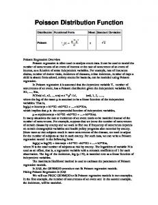
de Finetti measure and if the method correctly indicated the winner team as the team with higher probability of a win. Table 3 is ordered from home team with highest to smallest probability of win. The proportion of correct prediction was 70%. The teams with an estimated probability of win higher than 0.5, were the actual winning team. If we consider the probability of home team does not loss, i.e., probability of win or tie, then in 80% of games the method correctly indicates the home team as not losing. Figure 1 displays the graphic of attack versus defense effect. In this graphic, each dot (•) represent the attack and defense effect of each team. Manchester United and Liverpool have the highest effect attack; while Stoke City and West Ham United have the smallest effect attack. The Manchester City has the best defense effect, i.e., the smallest defense effect; decreasing the expected number of goals of the opposing team.. In opposite, Reading has the worst defense effect, i.e., the highest defense effect, which increases the expected number of goals of the opposing team. Using a simulation procedure, we estimate the number of points, the number of wins, draw and loss, number of goals for and against for each team. Table 4 presents these values and is organized by the real number of points for each team. The last column in Table 4 show the difference between number of goals for and against. Note that, the six teams with highest estimated number of points are really the six best teams of the championship.


304

Table 4: Predictions and real values Points Est. real Manchester United 92 89 Manchester City 74 78 Chelsea 71 75 Arsenal 71 73 Tottenham Hotspur 65 72 Everton 62 63 Liverpool 56 61 West Bromwich Albion 48 49 Swansea City 49 46 West Ham United 49 46 Norwich City 44 44 Fulham 42 43 Stoke City 42 42 Southampton 44 41 Aston Villa 44 41 Newcastle United 37 41 Sunderland 43 39 Wigan Athletic 35 36 Reading 32 28 Queens Park Rangers 30 25 Team

Won Est. real 29 28 22 23 20 22 20 21 18 21 16 16 14 16 14 14 12 11 13 12 10 10 10 11 09 09 10 09 11 10 10 11 11 09 09 09 07 06 05 04

Drawn Est. real 05 05 08 09 11 09 11 10 11 09 14 15 14 13 06 07 13 13 10 10 14 14 12 10 15 15 14 14 11 11 07 08 10 12 08 09 11 10 15 13

Lost Est. real 04 05 08 06 07 07 07 07 09 08 08 07 10 09 18 17 13 14 15 16 14 14 16 17 14 14 14 15 16 17 21 19 17 17 21 20 20 22 18 21

Goals for Est. real 88 86 64 66 75 75 68 66 65 66 57 55 69 71 48 53 50 47 45 45 38 41 49 50 35 34 50 49 46 47 44 45 46 41 43 47 48 43 31 30

Goals against Est. real 39 43 39 34 41 39 36 37 51 46 42 40 47 43 53 57 51 51 51 53 58 58 61 60 46 45 59 60 66 69 70 68 55 54 67 73 70 73 57 60

Difference of goals Est. real 49 43 25 32 34 36 32 35 14 20 15 15 22 28 −05 −04 −01 −04 −06 −08 −20 −17 −12 −10 −11 −11 −09 −11 −20 −22 −26 −23 −09 −13 −24 −26 −22 −30 −26 −30

Queens Park Rangers Reading Wigan Athletic Sunderland Newcastle Aston Villa Southampton Stoke City Fulham Norwich City West Ham United Swansea City West Bromwich Albion Liverpool Everton Tottenham Arsenal Chelsea Manchester City Manchester United 40

60

80

Figure 2: Box plot of number of points for R = 1,000 simulations.

100


305

Table 5: Probability to be the champion Rounds 20–38 22–38 24–38 26–38 28–38 30–38 32–38 34–38 36–38 38

Manchester United 0.708 0.662 0.990 0.988 0.873 0.996 0.981 0.998 1.000 1.000

Manchester City 0.235 0.297 0.007 0.012 0.127 0.003 0.018 0.002 0.000 0.000

Chelsea 0.025 0.001 0.003 0.000 0.000 0.001 0.001 0.000 0.000 0.000

Arsenal 0.002 0.000 0.000 0.000 0.000 0.000 0.000 0.000 0.000 0.000

Tottenham Hotspur 0.004 0.031 0.000 0.000 0.000 0.000 0.000 0.000 0.000 0.000

Everton 0.008 0.008 0.000 0.000 0.000 0.000 0.000 0.000 0.000 0.000

Liverpool 0.000 0.001 0.000 0.000 0.000 0.000 0.000 0.000 0.000 0.000

Table 6: Probability to classify for the UEFA Champions League Rounds 20–38 22–38 24–38 26–38 28–38 30–38 32–38 34–38 36–38 38

Manchester United 0.993 0.996 1.000 1.000 1.000 1.000 1.000 1.000 1.000 1.000

Manchester City 0.955 0.982 0.925 0.992 0.998 0.985 0.998 1.000 1.000 1.000

Chelsea 0.617 0.402 0.851 0.693 0.823 0.873 0.673 0.697 0.905 1.000

Arsenal 0.160 0.117 0.203 0.268 0.344 0.148 0.646 0.683 0.527 1.000

Tottenham 0.337 0.778 0.290 0.799 0.773 0.608 0.543 0.542 0.519 0.000

Everton 0.276 0.506 0.323 0.052 0.012 0.256 0.128 0.078 0.049 0.000

Liverpool 0.000 0.095 0.257 0.157 0.013 0.100 0.011 0.000 0.000 0.000

Reading 0.813 0.621 0.663 0.643 0.711 0.796 0.874 0.986 1.000 1.000

Queens P.R. 0.591 0.917 0.489 0.580 0.812 0.869 0.943 0.999 1.000 1.000

Table 7: Probability of to be relegated to the second division Round 20–38 22–38 24–38 26–38 28–38 30–38 32–38 34–38 36–38 38

Stoke City 0.000 0.004 0.010 0.007 0.034 0.008 0.007 0.153 0.000 0.000

Southampton 0.078 0.495 0.173 0.341 0.095 0.323 0.020 0.004 0.001 0.000

Aston Villa 0.116 0.121 0.368 0.406 0.719 0.314 0.213 0.217 0.102 0.000

Newcastle U. 0.250 0.053 0.100 0.001 0.093 0.063 0.030 0.028 0.115 0.000

Sunderland 0.250 0.240 0.072 0.039 0.015 0.076 0.199 0.119 0.027 0.000

Wigan A. 0.440 0.410 0.779 0.864 0.342 0.484 0.624 0.432 0.720 1.000

Figure 2 shows box plot of the estimated points for the 20 teams from R = 1,000 simulations. As we can note, the simulation results show Manchester United as champion.

3.2. Predictions for whole second phase We apply the proposed method to predict results of the matches of rounds 20 to 38. Using a simulation procedure, we calculated the probability of each team being the champion and to classify the Union of European Football Associations (UEFA) champions league. Tables 5–7 below show results for rounds 20, 22, 24, . . . , 38. Tables B.1–B.3 in Appendix B of the SM show results for all rounds. Table 5 shows the rounds simulated and the probabilities to be champion for the seven teams with the highest number of goals scored (Table 1). In all second phase of the champion the method indicates Manchester United as the champion with a probability higher


306

Table 8: Number of games and goals scored by each team at home and away in each phase of the BFL 1st phase Games Games Goals Goals at home away Corinthians 09 17 10 10 Atlético-MG 10 19 09 14 Palmeiras 10 19 09 13 Santos 09 16 10 09 São Paulo 10 16 09 09 Sport 10 18 09 13 Grêmio 10 21 09 08 Flamengo 09 12 10 09 Cruzeiro 09 08 10 07 Atlético Paranaense 10 14 09 09 Ponte Preta 09 09 10 12 Fluminense 10 12 09 10 Internacional 09 09 10 05 Goiás 09 08 10 08 Ava´ı 10 13 09 05 Figueirense 09 10 10 08 Chapecoense 10 14 09 03 Coritiba 09 08 10 05 Vasco da Gama 10 05 09 03 Joinvile 09 09 10 04 Team

2nd phase Games Games Goals Goals at home away 10 24 09 20 09 17 10 15 09 12 10 16 10 31 09 03 09 19 10 09 09 15 10 07 09 14 10 09 10 16 09 08 10 20 09 09 09 16 10 04 10 13 09 07 09 13 10 05 10 19 09 06 10 14 09 09 09 13 10 07 10 08 09 10 09 09 10 08 10 07 09 11 09 08 10 12 10 10 09 03

Number of goals At home Away Total 41 36 31 47 35 33 35 28 28 30 22 25 28 22 26 18 23 15 13 19

30 29 29 12 18 20 17 17 16 13 19 15 11 17 12 18 11 16 15 07

71 65 60 59 53 53 52 45 44 43 41 40 39 39 38 36 34 31 28 26

than 0.63. After the 28th round, the probability of Manchester United be the champion is higher than 0.99. Table 6 shows the probabilities for the seven teams with highest number of goals to classify for the UEFA Champions League. In all second phase, Manchester United has a probability to classify to the UEFA Champions League that is higher than 0.99. After 28th round the probability of Manchester City to classify is higher than 0.99. Six rounds before the ending of the champion, the method indicates Manchester United and Manchester City as the two teams classified for the UEFA Champions League. Table 7 shows the probabilities of the eight teams with smallest estimated number of points to be relegated to the second division (Table 4). In the 35th round (four rounds before the end of the championship), the method indicates these both teams as the teams relegated to the second division. Figures C.1 and C.2 in Appendix C of the SM shows the attack effect and defense effect for the best four teams of the EPL in the 20–38 rounds.

4. Application 2 In this section we apply the proposed method to the BFL. As EPL, the BFL it is also composed by n + 1 = 20 teams. The games are played in two phases, in which each team plays 19 games by phase. At the end of the 38 rounds, the team with highest number of points is champion; the four teams with the highest number of points are classified to 2016 Copa Libertadores of América and the four teams with the smallest points are relegated to the second division of the BFL. Table 8 shows the number of games and the number of goals scored by each team at home and away in each phase of the BFL. The two best team of BFL, Corinthians and Atlético-MG, have the highest number of goals scored; being that the best team, Corinthians, has the highest number of goals scored at home and away. The two worst teams of the BFL, Joinvile and Vasco, are the teams with smallest number of goals scored. Joinvile has the smallest number of goals scored away, while Vasco


307

Table 9: Number of games ended with number of goals (xt , x s ), for xt , x s ∈ {0, 1, 2, 3, +4} Away team 0 1 2 3 +4 Total

0 39 27 16 5 1 88

1 56 33 21 11 4 125

Home team 2 35 43 16 4 0 98

3 28 15 5 3 0 51

+4 4 10 3 1 0 18

Total

de Finetti

Correct

162 128 61 24 5 380

Table 10: Probabilities of win, draw and loss for each match of the 27th round Home

Away

Palmeiras Internacional Ponte Preta Corinthians Goiás Vasco Atlético-MG Ava´ı Coritiba Chapecoense

Grêmio Figueirense Fluminense Santos Joinvile Sport Flamengo São Paulo Atlético-PR Cruzeiro

Win 0.590 0.324 0.499 0.576 0.766 0.607 0.573 0.337 0.387 0.484

Probability Draw 0.256 0.228 0.233 0.208 0.136 0.222 0.226 0.332 0.292 0.262

Loss 0.154 0.448 0.268 0.216 0.098 0.172 0.201 0.331 0.321 0.254

Score 3–2 1–1 3–1 2–0 3–0 2–1 4–1 2–1 2–0 0–2

0.258 0.903 0.377 0.270 0.083 0.233 0.273 0.659 0.564 0.859

Yes No Yes Yes Yes Yes Yes Yes Yes No

has the smallest number of goals scored at home. Table 9 presents the number of games that end with the number of goals (xt , x s ). In 52.63% of the games the home team was the winner; in 23.42% the winner was the away team and in 23.95% the game ended in a draw. The amount of victory of the home team is more than twice the amount of victories for the away team. The two most frequent results was 1–0 (56 games) and 2–1 (43 games) for the home team.

4.1. Prediction for a round Here we present the predictions of the 27th round of the BFL. Table 10 presents the probabilities of win, draw, goals scored, de Finetti measure and if the method indicates the winning team as the team with higher probability of win. The percentage of correct predictions was 80%. Figure 3 displays the graphic of attack versus defense effect. Palmeiras, Atlético-MG and Corinthians have the highest attack effect. Table 10 shows that these teams won their games. Chapecoense, Internacional and Joinvile have the worst attack effect. Corinthians also presents the better defense effect, while Vasco, Ava´ı and Figueirense have the worst defense effect. Using the simulation procedure, we estimate the number of points for each team. Figure 4 shows box plot of the estimated points for the 20 teams of the BFL from R = 1,000 simulations. As we can note, the simulation results show Corinthians as the champion. Corinthians, Atlético-MG, Grêmio and São Paulo as teams classified for 2016 Copa Libertadores of América; and Vasco, Joinvile, Figueirense and Goiás as teams relegated to the second division. From real results, the method correctly indicates the champion, the four teams classified for 2016 Copa Libertadores of América; and the three teams relegated to the second division: Vasco, Joinvile and Goiás. The fourth team relegated to the second division was Ava´ı and not Figueirense as foreseen by the method.


0.4

308

Vasco da Gama Avaí

Flamengo Santos Fluminense Ponte PretaPalmeiras

0.0

Atlético−PR

−0.2

Internacional Chapecoense

Cruzeiro Joinville

Atlético−MG São Paulo Sport Recife

Coritiba

Goiás Grêmio Corinthians

−0.4

Defensive Effect

0.2

Figueirense

−0.5

0.0

0.5

Attack Effect

Figure 3: Attack and defense effect.

Joinville Goiás Vasco da Gama Avaí Figueirense Coritiba Chapecoense Fluminense Flamengo Ponte Preta Atlético−PR Palmeiras Cruzeiro Santos Sport Recife Internacional São Paulo Grêmio Atlético−MG Corinthians 20

40

60

80

Figure 4: Box plot of number of points for R = 1,000 simulations.


309

Table 11: Probability to be the champion Rounds 20–38 22–38 24–38 26–38 28–38 30–38 32–38 34–38 36–38 38

Corinthians 0.572 0.176 0.692 0.579 0.945 0.728 0.940 0.999 1.000 1.000

Atlético-MG 0.047 0.204 0.086 0.380 0.035 0.230 0.058 0.001 0.000 0.000

Grêmio 0.065 0.185 0.194 0.025 0.007 0.012 0.002 0.000 0.000 0.000

São Paulo 0.125 0.007 0.020 0.010 0.002 0.020 0.000 0.000 0.000 0.000

Internacional 0.000 0.031 0.000 0.000 0.000 0.000 0.000 0.000 0.000 0.000

Sport Recife 0.008 0.028 0.006 0.000 0.002 0.000 0.000 0.000 0.000 0.000

Santos 0.000 0.002 0.000 0.002 0.001 0.007 0.000 0.000 0.000 0.000

Sport Recife 0.135 0.178 0.274 0.010 0.251 0.002 0.034 0.200 0.037 0.030

Santos 0.003 0.030 0.011 0.164 0.204 0.345 0.203 0.460 0.390 0.000

Table 12: Probability to classify for the 2016 Copa Libertadores of América Rounds 20–38 22–38 24–38 26–38 28–38 30–38 32–38 34–38 36–38 38

Corinthians 0.953 0.606 0.991 0.992 0.999 0.996 1.000 1.000 1.000 1.000

Atlético-MG 0.467 0.676 0.856 0.981 0.751 0.942 0.997 1.000 1.000 1.000

Grêmio 0.487 0.573 0.943 0.712 0.540 0.456 0.927 0.971 1.000 1.000

São Paulo 0.684 0.048 0.548 0.399 0.231 0.587 0.330 0.140 0.488 0.859

Internacional 0.000 0.231 0.032 0.025 0.100 0.101 0.131 0.123 0.014 0.111

Table 13: Probability of to be relegated to the second division Round 20–38 22–38 24–38 26–38 28–38 30–38 32–38 34–38 36–38 38

Joinville 0.381 0.462 0.782 0.800 0.882 0.978 0.645 0.977 0.999 1.000

Goiás 0.330 0.703 0.509 0.155 0.378 0.449 0.646 0.407 0.915 0.949

Vasco da Gama 0.301 0.981 0.995 0.996 0.987 0.869 0.954 0.982 0.971 0.911

Ava´ı 0.513 0.535 0.664 0.272 0.506 0.120 0.799 0.625 0.443 0.421

Figueirense 0.317 0.103 0.111 0.264 0.662 0.491 0.254 0.081 0.086 0.711

Coritiba 0.798 0.306 0.151 0.208 0.084 0.635 0.601 0.830 0.581 0.008

4.2. Predictions for whole second phase In this section, we apply the proposed method to predict results of the matches of rounds 20 to 38. Table 11 shows the rounds simulated and the probabilities to be champion for the seven teams with the highest estimated number of points. After 31-round the method indicates Corinthians as the champion with a probability higher than 0.93. The method indicates the Corinthians as the champion three rounds before the ending. Table 12 shows the probabilities for the seven teams with the highest estimated number of points to classify for the 2016 Copa Libertadores of América. Eight rounds before the ending of the BFL, the probability of the Corinthians and Atlético-MG to classify for the 2016 Copa Libertadores of América is higher than 0.990. Three rounds before the ending of the champion, the method indicates the Corinthians, Atlético-MG and Grêmio as teams classified 2016 Copa Libertadores of América. In

310


the last round, the method indicates São Paulo as the fourth team classified with the probability 0.859. Table 13 shows the probabilities of the six teams with smallest estimated number of points to be relegated to the second division. Three rounds before the ending of the champion, the method indicates the Joinvile, Goiás and Vasco as teams relegated to the second division with a probability higher than 0.90. In the last round, the method indicates Ava´ı and Figueirense with probabilities 0.421 and 0.711 to be relegated. The Ava´ı was relegated. Tables D.1–D.3 in Appendix D of the show results for all rounds. Figures E.1 and E.2 in Appendix E of the SM show, respectively, the attack effect and defense effect for the best four teams and worst four teams of the BFL in the 20–38 rounds.

5. Final remarks In this paper, we develop a model to estimate the probabilities of win, tie and defeat in football games. In order to calculate these probabilities we propose a Poisson regression model, in which, the average of goals scored reflects the strength of attack of the team, the strength of defense of the opposing team and the home team effect. Inferences on parameters of interest were done via Bayesian inference. The accuracy of the forecasts were measured using the de Finetti measure. In order to illustrate the application of the proposed method, we apply it to the 2012–2013 EPL and to 2015 BFL. Using a simulation procedure, we calculated satisfactory results on the probability of each team being the champion and classify the continental tournaments. The method correctly indicated the champion of the EPL and BFL with three rounds before the ending of the championship. The method also correctly indicates the teams classified for the continental tournaments. We also present the probabilities of the teams to be relegated to the second division. Again, the method presents satisfactorily results. The attack effect and defense effect for the best four teams and worst four teams of the EPL and BFL in the 20–38 rounds were also presented. Results showed that champions team have a higher attack effect and smaller defense effect. These two facts, increase in the expected number of goals of the champion team and decrease the expected number of goals of an opposing team, respectively. Results obtained show that proposed method may be an effective alternative to predict football outcomes. A practical differential of the proposed method is its simplicity to be implemented in software like OpenBUGS and R. We have developed a Poisson regression model based on the average of goals scored that reflect the strength of attack and defense of the teams; in addition, the model can also describe the means of goals scored using other covariates, such as, atmospheric condition, injuries, suspensions, tactical scheme, and crisis. It can be seems as future work. Besides, the method can be easily used for the analysis of the upcoming championship season and adapted to other championship and tournaments with different forms of dispute. All computational were performed using OpenBUGS and R systems via R2WinBUGS package. The computer programs are also available in the Supplementary Material at CSAM homepage (http://csam.or.kr).

Acknowledgements We thank the Editor and the referees for their comments, suggestions and criticisms which have led to improvements in this article. The first author acknowledges the Brazilian institution CNPq. The research of Francisco Louzada is supported by CNPq and FAPESP.


311

Appendix Here we provide some additional results and the computational codes developed to calculate the probabilities presented in the manuscript.

Appendix A: Estimations of βs In this appendix we present some details of the estimation procedure of parameters βk = (βk0 , βka , βkd , βkh ), for k = t, s. From model (2.1) of the manuscript, the likelihood function is given by L(βt , β s |xt , xs ) =

U β nr ∏ ∏ e xkm Ukm βk e−e km k

k∈{t,s} m=1

xkm !

.

(A.1)

The log-likelihood function is given in equation (2.3) of the manuscript. We assume that priors are a priori independent, i.e., π(βt , β s ) = π(βt )π(β s ), in which, π(βk ) = π(βk0 )π(βka )π(βkd )π(βkh ), for k = t, s. So, we consider the following prior distributions: ( ) βk0 ∼ N 0, 10−4 ,

( ) βka ∼ N 0, 10−3 ,

( ) βkc d ∼ N 0, 10−3

and

( ) βkh ∼ N 0, 10−3 ,

for k = t, s, where N(0, b) denotes the normal distribution with mean 0 and precision b. Here, we present the joint posterior distribution for parameters βt . The joint posterior distribution for β s is obtained in a similar way. Updating the joint prior distribution for π(βt ) via likelihood function in (A.1), the joint posterior distribution is given by  nr  ∏ x U β −eUtm βt  tm tm t   π(βt0 )π(βta )π(β sd )π(βth ). π(βt |xt ) ∝  e e

(A.2)

m=1

The conditional posterior distributions for βtw , w ∈ {0, a, d, h}, is given by   nr ∏ x U β −eUtm βt   π(βtw ), e tm tm t e π(βtw |xt , βt \ βtw ) ∝  m=1

where βt \ βtw denotes the vector βt excluding βtw . As one can note, the conditional posterior distribution for βt0 , βta , β sd and βth do not follow any close distribution. For this case, the usual Bayesian procedure to generate random samples from posterior distribution is to use the Metropolis-Hastings (MH) algorithm. The Metropolis-Hastings algorithm together with the Gibbs sampling are the two most popular examples of a Markov chain Monte Carlo (MCMC) method. This algorithm is used for sampling from generic distributions if we do not know how to generate a random sample. Similar to acceptancerejection sampling, the MH algorithm considers that (to each iteration of the algorithm) a candidate value can be generated from a proposal density; therefore, the candidate value is accepted according to an adequated acceptance probability. This procedure guarantees the convergency of the Markov chain for the target density. For more details on MH algorithm see Hastings (1970), Chib and Greenberg (1995), Gelman et al. (1995) and Gilks et al. (1996).


312

Table B.1: Probability to be the champion Rounds 20–38 21–38 22–38 23–38 24–38 25–38 26–38 27–38 28–38 29–38 30–38 31–38 32–38 33–38 34–38 35–38 36–38 37–38 38

Manchester United 0.708 0.815 0.662 0.925 0.990 0.633 0.988 0.972 0.873 0.995 0.996 0.993 0.981 0.989 0.998 1.000 1.000 1.000 1.000

Manchester City 0.235 0.031 0.297 0.015 0.007 0.345 0.012 0.006 0.127 0.004 0.003 0.007 0.018 0.011 0.002 0.000 0.000 0.000 0.000

Chelsea 0.025 0.129 0.001 0.001 0.003 0.008 0.000 0.009 0.000 0.000 0.001 0.000 0.001 0.000 0.000 0.000 0.000 0.000 0.000

Arsenal 0.002 0.001 0.000 0.000 0.000 0.000 0.000 0.000 0.000 0.000 0.000 0.000 0.000 0.000 0.000 0.000 0.000 0.000 0.000

Tottenham Hotspur 0.004 0.020 0.031 0.045 0.000 0.005 0.000 0.013 0.000 0.001 0.000 0.000 0.000 0.000 0.000 0.000 0.000 0.000 0.000

Everton 0.008 0.000 0.008 0.004 0.000 0.009 0.000 0.000 0.000 0.000 0.000 0.000 0.000 0.000 0.000 0.000 0.000 0.000 0.000

Liverpool 0.000 0.000 0.001 0.000 0.000 0.000 0.000 0.000 0.000 0.000 0.000 0.000 0.000 0.000 0.000 0.000 0.000 0.000 0.000

For example, to update parameter βth via MH algorithm, consider (βt0 , βta , β sd , βth ) be the current state of the Markov chain. Let β∗th be a candidate value generated from a candidate generating-density distribution q[β∗th |βth ]. So, the value β∗th is accepted with probability Ψ(β∗th |βth ) = min(1, Aβth ), where ( ) ( ) [ ] L βt0 , βta , β sd , β∗th |xt π β∗th q βth |β∗th Aβth = ( (A.3) ) ( ) [ ] L βt0 , βta , β sd , βth |xt π βth q β∗th |βth ∏ r xtm Utm βt −eUtm βt e e ] is the likelihood function for βt . and L(βt0 , βta , β sd , βth |xt ) ∝ [ nm=1 In practical terms, the MH algorithm is implemented as follows. (l) (l) Metropolis-Hastings algorithm: Let the current state of the Markov chain consist of (β(l) t0 , βta , β sd , (l−1) βth ), where l is lth iteration of the algorithm, for l = 1, . . . , L. So, update βth as follows:

(1) Generate β∗th ∼ q[β∗th |βth ]; (2) Calculate Ψ(β∗th |βth ) = min(1, Aβth ), where Aβth is given in (A.3); ∗ ∗ (3) Generate u ∼ U(0, 1). If u ≤ Ψ(β∗th |βt h) accept β∗th and do β(l) th = βth . Otherwise, reject βth and do (l) (l−1) βth = βth .

The procedure to update βt0 , βta and β sd is similar to described to parameter βth . We implement the MH in order to generate random samples from posterior distribution in (A.2) using the WinBUGS (Spiegelhalter et al., 2003) and R (R Development Core Team, 2012) softwares via R2WinBUGS package Gelman et al. (2006). The computer programs are available in the Supplementary Material at CSAM homepage (http://csam.or.kr).

Appendix B: Estimated probabilities for EPL In this appendix we present the complete version of the Tables 5–7 showed in manuscript. Tables B.1 and B.2 show all rounds simulated, the probabilities to be champion and to classify for the continental


313

Table B.2: Probability to classify for the UEFA Champions League Rounds 20–38 21–38 22–38 23–38 24–38 25–38 26–38 27–38 28–38 29–38 30–38 31–31 32–38 33–38 34–38 35–38 36–38 37–38 38

Manchester United 0.993 0.998 0.996 0.998 1.000 1.000 1.000 1.000 1.000 1.000 1.000 1.000 1.000 1.000 1.000 1.000 1.000 1.000 1.000

Manchester City 0.955 0.701 0.982 0.724 0.925 0.993 0.992 0.848 0.998 0.995 0.985 0.975 0.998 1.000 1.000 1.000 1.000 1.000 1.000

Chelsea 0.617 0.918 0.402 0.297 0.851 0.528 0.693 0.880 0.823 0.802 0.873 0.927 0.673 0.965 0.697 0.810 0.905 0.961 1.000

Arsenal 0.160 0.081 0.117 0.153 0.203 0.046 0.268 0.189 0.344 0.033 0.148 0.170 0.646 0.332 0.683 0.737 0.527 0.775 1.000

Tottenham 0.337 0.591 0.778 0.896 0.290 0.547 0.799 0.905 0.773 0.776 0.608 0.774 0.543 0.655 0.542 0.425 0.519 0.264 0.000

Everton 0.276 0.213 0.506 0.284 0.323 0.552 0.052 0.076 0.012 0.159 0.256 0.079 0.128 0.037 0.078 0.028 0.049 0.000 0.000

Liverpool 0.000 0.034 0.095 0.017 0.257 0.297 0.157 0.009 0.013 0.214 0.100 0.069 0.011 0.011 0.000 0.000 0.000 0.000 0.000

Table B.3: Probability of to be relegated to the second division Round Stoke City Southampton Aston Villa Newcastle United Sunderland Wigan Athletic Reading Queens P.R. 20–38 0.000 0.078 0.116 0.250 0.250 0.440 0.813 0.591 21–38 0.006 0.308 0.042 0.262 0.294 0.073 0.863 0.754 22–38 0.004 0.495 0.121 0.053 0.240 0.410 0.621 0.917 23–38 0.068 0.015 0.386 0.597 0.121 0.214 0.976 0.162 24–38 0.010 0.173 0.368 0.100 0.072 0.779 0.663 0.489 25–38 0.005 0.345 0.456 0.387 0.084 0.495 0.178 0.846 26–38 0.007 0.341 0.406 0.001 0.039 0.864 0.643 0.580 27–38 0.000 0.076 0.165 0.666 0.180 0.339 0.484 0.855 28–38 0.034 0.095 0.719 0.093 0.015 0.342 0.711 0.812 29–38 0.011 0.216 0.867 0.147 0.016 0.338 0.570 0.751 30–38 0.008 0.323 0.314 0.063 0.076 0.484 0.796 0.869 31–38 0.021 0.201 0.252 0.018 0.127 0.439 0.923 0.968 32–38 0.007 0.020 0.213 0.030 0.199 0.624 0.874 0.943 33–38 0.070 0.003 0.250 0.010 0.291 0.373 0.985 0.975 34–38 0.153 0.004 0.217 0.028 0.119 0.432 0.986 0.999 35–38 0.014 0.003 0.290 0.040 0.072 0.554 1.000 1.000 36–38 0.000 0.001 0.102 0.115 0.027 0.720 1.000 1.000 37–38 0.000 0.005 0.004 0.131 0.024 0.620 1.000 1.000 38 0.000 0.000 0.000 0.000 0.000 1.000 1.000 1.000

championship for the seven teams with the highest number of goals scored. Table B.3 shows all rounds simulated and the probabilities of the eight teams with smallest estimated number of points to be relegated to the second division.

Appendix C: Attack and defense effect for EPL In this appendix we present the attack and defense effect for the best four teams and worst four teams of the EPL and BFL in the 20–38 rounds. Figure C.1 shows the attack effect and defense effect for the best four teams of the EPL in the


0.0

Offensive Effect

0.5

1.0

314

Manchester United −0.5

Manchester City Chelsea

−1.0

Arsenal

20

25

30

35

1.0

Rounds

Manchester United Manchester City 0.5

Chelsea

0.0 −1.0

−0.5

Defensive Effect

Arsenal

20

25

30

35

Rounds

Figure C.1: Attack and defense effect of the best four teams in rounds 20–38.

20–38 rounds. These four teams present positive attack. Manchester City, Chelsea and Arsenal have negative defense affect in the 20–38 rounds. The positive attack increases the expected number of goals of the teams and the negative defense attack decrease the expected number of goals of the opposing team. In opposite, the two worst team of the EPL, Queens Park Rangers and Reading have negative attack effect and positive defense attack, as showed in Figure C.2. This Figure C.2 also show the


1.0

315

Queens Park Rangers Reading 0.5

Wigan Athletic

0.0 −1.0

−0.5

Offensive Effect

Sunderland

20

25

30

35

0.0

Queens Park Rangers

−0.5

Defensive Effect

0.5

1.0

Rounds

Reading Wigan Athletic

−1.0

Sunderland

20

25

30

35

Rounds

Figure C.2: Attack and defense effect of the worst four teams in rounds 20–38.

attack and defense effect for Wigan Athletic and Sunderland.

Appendix D: Estimated probabilities for BFL In this appendix we present the complete version of the Tables 11–13 showed in manuscript. Tables D.1 and D.2 show all rounds simulated, the probabilities to be champion and to classify for the

316


Table D.1: Probability to be the champion Rounds simulated 20–38 21–38 22–38 23–38 24–38 25–38 26–38 27–38 28–38 29–38 30–38 31–38 32–38 33–38 34–38 35–38 36–38 37–38 38

Corinthians 0.572 0.343 0.176 0.465 0.692 0.386 0.579 0.430 0.945 0.953 0.728 0.439 0.940 0.953 0.999 0.999 1.000 1.000 1.000

Atlético-MG 0.047 0.298 0.204 0.199 0.086 0.388 0.380 0.505 0.035 0.040 0.230 0.394 0.058 0.047 0.001 0.001 0.000 0.000 0.000

Grêmio 0.065 0.214 0.185 0.290 0.194 0.099 0.025 0.048 0.007 0.007 0.012 0.166 0.002 0.000 0.000 0.000 0.000 0.000 0.000

São Paulo 0.125 0.073 0.007 0.016 0.020 0.002 0.010 0.002 0.002 0.000 0.020 0.000 0.000 0.000 0.000 0.000 0.000 0.000 0.000

Internacional 0.000 0.000 0.031 0.000 0.000 0.016 0.000 0.005 0.000 0.000 0.000 0.000 0.000 0.000 0.000 0.000 0.000 0.000 0.000

Sport Recife 0.008 0.010 0.028 0.001 0.006 0.000 0.000 0.002 0.002 0.000 0.000 0.000 0.000 0.000 0.000 0.000 0.000 0.000 0.000

Santos 0.000 0.030 0.002 0.015 0.000 0.000 0.002 0.004 0.001 0.000 0.007 0.000 0.000 0.000 0.000 0.000 0.000 0.000 0.000

Sport Recife 0.135 0.206 0.178 0.054 0.274 0.008 0.010 0.114 0.251 0.067 0.002 0.045 0.034 0.417 0.200 0.183 0.037 0.008 0.030

Santos 0.003 0.359 0.030 0.296 0.011 0.008 0.164 0.322 0.204 0.237 0.345 0.296 0.203 0.396 0.460 0.547 0.390 0.281 0.000

Table D.2: Probability to classify for the 2016 Copa Libertadores of América Rounds simulated 20–38 21–38 22–38 23–38 24–38 25–38 26–38 27–38 28–38 29–38 30–38 31–38 32–38 33–38 34–38 35–38 36–38 37–38 38

Corinthians 0.953 0.865 0.606 0.951 0.991 0.936 0.992 0.983 0.999 1.000 0.996 0.999 1.000 1.000 1.000 1.000 1.000 1.000 1.000

Atlético-MG 0.467 0.821 0.676 0.875 0.856 0.926 0.981 0.981 0.751 0.969 0.942 0.999 0.997 0.999 1.000 1.000 1.000 1.000 1.000

Grêmio 0.487 0.765 0.573 0.884 0.943 0.683 0.712 0.709 0.540 0.894 0.456 0.990 0.927 0.873 0.971 0.962 1.000 1.000 1.000

São Paulo 0.684 0.441 0.048 0.272 0.548 0.117 0.399 0.156 0.231 0.105 0.587 0.173 0.330 0.097 0.140 0.213 0.488 0.314 0.859

Internacional 0.000 0.001 0.231 0.039 0.032 0.299 0.025 0.255 0.100 0.011 0.101 0.029 0.131 0.184 0.123 0.064 0.014 0.367 0.111

continental championship for the seven teams with the highest number of goals scored. Table D.3 shows the probabilities of the six teams with smallest estimated number of points to be relegated to the second division.

Appendix E: Attack and defense effect for BFL In this appendix we present the attack and defense effect for the best four and worst four teams of the BFL in the 20–38 rounds. Figures E.1 and E.2 show, respectively, the attack effect and defense effect for the best four teams


317

Table D.3: Probability of to be relegated to the second division Joinville 0.381 0.923 0.462 0.842 0.782 0.701 0.800 0.940 0.882 0.600 0.978 0.904 0.645 0.859 0.977 0.909 0.999 1.000 1.000

Goiás 0.330 0.528 0.703 0.262 0.509 0.152 0.155 0.337 0.378 0.726 0.449 0.565 0.646 0.762 0.407 0.626 0.915 0.953 0.949

Vasco da Gama 0.301 0.983 0.981 0.910 0.995 0.728 0.996 0.948 0.987 0.917 0.869 0.944 0.954 0.942 0.982 0.856 0.971 0.864 0.911

Ava´ı 0.513 0.053 0.535 0.629 0.664 0.536 0.272 0.419 0.506 0.547 0.120 0.274 0.799 0.317 0.625 0.701 0.443 0.651 0.421

Figueirense 0.317 0.628 0.103 0.369 0.111 0.174 0.264 0.802 0.662 0.618 0.491 0.509 0.254 0.505 0.081 0.169 0.086 0.246 0.711

0.0

Offensive Effect

0.5

1.0

Round simulated 20–38 21–38 22–38 23–38 24–38 25–38 26–38 27–38 28–38 29–38 30–38 31–38 32–38 33–38 34–38 35–38 36–38 37–38 38

Corinthians −0.5

Atlético−MG Grêmio

−1.0

São Paulo

20

25

30

35

1.0

Rounds

Corinthians Atlético−MG 0.5

Grêmio

0.0 −1.0

−0.5

Defensive Effect

São Paulo

20

25

30

35

Rounds

Figure E.1: Attack and defense effect of the best four teams in rounds 20–38.

Coritiba 0.798 0.217 0.306 0.416 0.151 0.553 0.208 0.155 0.084 0.124 0.635 0.441 0.601 0.431 0.830 0.739 0.581 0.286 0.008


1.0

318

Joinville Goiás 0.5

Vasco da Gama

0.0 −1.0

−0.5

Offensive Effect

Avaí

20

25

30

35

1.0

Rounds

Zaragoza Deportivo La Coruña Mallorca

0.0 −1.0

−0.5

Defensive Effect

0.5

Celta de Vigo

20

25

30

35

Rounds

Figure E.2: Attack and defense effect of the worst four teams in rounds 20–38.

and worst four teams of the BFL in the 20–38 rounds. Corinthians and Atlético-MG have the highest attack effect. Corinthians also have the best defense effect. After 32-round Corinthians is the team with the best attack and defense effect. The four worst teams of BFL have an attack effect, meaning a low expected number of goals and few amount of victories that regulates these teams to the second division.

References Baio G and Blangiardo M (2010). Bayesian hierarchical model for the prediction of football result, Journal of Applied Statistics, 37, 253–264. Bastos LS and da Rosa JMC (2013). Predicting probabilities for the 2010 FIFA world cup games using a Poisson-Gamma model, Journal of Applied Statistics, 40, 1533–1544. Brillinger DR (2008). Modelling game outcomes of the Brazilian 2006 series a championship as ordinal-valued, Brazilian Journal of Probability Statistics, 22, 89–104.


319

Chib S and Greenberg E (1995). Understanding the Metropolis-Hastings algorithm, The American Statistician, 49, 327–335. Dixon MJ and Coles SG (1997). Modelling association football scores and inefficiencies in the football betting market, Journal of the Royal Statistical Society: Series C (Applied Statistics), 46, 265–280. Dyte D and Clarke SR (2000). A ratings based Poisson model for World Cup soccer simulation, Journal of the Operational Research Society, 51, 993–998. Gelman A, Carlin JB, Stern HS, and Rubin DB (1995). Bayesian Data Analysis, Chapman and Hall, London. Gelman A, Sturtz S, Ligges U, Gorjane G, and Kerman J (2006). The R2WinBUGS Package Manual Version 2.0-4, Statistic Department Faculty, New York. Gilks WR, Richardson S, and Spiegelhalter DJ (1996). Markov Chain Monte Carlo in Practice, Chapman and Hall, London. Hastings WK (1970). Monte Carlo sampling methods using Markov Chains and their applications, Biometrika, 57, 97–109. Karlis D and Ntzoufras I (2003). Analysis of sports data by using bivariate Poisson models, Journal of the Royal Statistical Society: Series D (The Statistician), 52, 381–393. Karlis D and Ntzoufras I (2009). Bayesian modelling of football outcomes: using the Skellam’s distribution for the goal difference, IMA Journal of Management Mathematics, 20, 133–145. Keller JB (1994). A characterization of the Poisson distribution and the probability of winning a game, The American Statistician, 48, 294–298. Knorr-Held L (2000). Dynamic rating of sports teams, Journal of the Royal Statistical Society: Series D (The Statistician), 49, 261–276. Koopman SJ and Lit R (2015). A dynamic bivariate Poisson model for analysing and forecasting match results in the English Premier League, Journal of the Royal Statistical Society: Series A (Statistics in Society), 178, 167–186. Lee AJ (1997). Modeling scores in the Premier League: is Manchester United really the best?, Chance, 10, 15–19. Maher MJ (1982). Modeling association football scores, Statistica Neerlandica, 36, 109–118. R Development Core Team (2012). R: A Language and Environment for Statistical Computing, R Foundation for Statistical Computing, Vienna, Austria. Spiegelhalter DJ, Thomas A, Best NG, and Lunn D (2003). WinBUGS User Manual (Version 1.4.1), MRC Biostatistics Unit, Cambridge, UK. Suzuki AK, Salasar LEB, Leite JG, and Louzada-Neto F (2010). A Bayesian approach for predicting match outcomes: the 2006 (Association) Football World Cup, Journal of the Operational Research Society, 61, 1530–1539. Volf P (2009). A random point process model for the score in sport matches, IMA Journal of Management Mathematics, 20, 121–131. Received May 5, 2016; Revised May 26, 2016; Accepted May 30, 2016