Revised November 2003
•
NREL/CP-550-33601
Predicting Long-Term Performance of Photovoltaic Arrays Using Short-Term Test Data and an Annual Simulation Tool Preprint G. Barker Mountain Energy Partnership Longmont, Colorado
P. Norton National Renewable Energy Laboratory
To be presented at the Solar 2003 Conference: America’s Secure Energy Austin, Texas June 21–26, 2003
National Renewable Energy Laboratory 1617 Cole Boulevard Golden, Colorado 80401-3393 NREL is a U.S. Department of Energy Laboratory Operated by Midwest Research Institute • Battelle • Bechtel Contract No. DE-AC36-99-GO10337
NOTICE The submitted manuscript has been offered by an employee of the Midwest Research Institute (MRI), a contractor of the US Government under Contract No. DE-AC36-99GO10337. Accordingly, the US Government and MRI retain a nonexclusive royalty-free license to publish or reproduce the published form of this contribution, or allow others to do so, for US Government purposes. This report was prepared as an account of work sponsored by an agency of the United States government. Neither the United States government nor any agency thereof, nor any of their employees, makes any warranty, express or implied, or assumes any legal liability or responsibility for the accuracy, completeness, or usefulness of any information, apparatus, product, or process disclosed, or represents that its use would not infringe privately owned rights. Reference herein to any specific commercial product, process, or service by trade name, trademark, manufacturer, or otherwise does not necessarily constitute or imply its endorsement, recommendation, or favoring by the United States government or any agency thereof. The views and opinions of authors expressed herein do not necessarily state or reflect those of the United States government or any agency thereof. Available electronically at http://www.osti.gov/bridge
Available for a processing fee to U.S. Department of Energy and its contractors, in paper, from: U.S. Department of Energy Office of Scientific and Technical Information P.O. Box 62 Oak Ridge, TN 37831-0062 phone: 865.576.8401 fax: 865.576.5728 email:
[email protected] Available for sale to the public, in paper, from: U.S. Department of Commerce National Technical Information Service 5285 Port Royal Road Springfield, VA 22161 phone: 800.553.6847 fax: 703.605.6900 email:
[email protected] online ordering: http://www.ntis.gov/ordering.htm
Printed on paper containing at least 50% wastepaper, including 20% postconsumer waste
PREDICTING LONG-TERM PERFORMANCE OF PHOTOVOLTAIC ARRAYS
USING SHORT-TERM TEST DATA AND AN ANNUAL SIMULATION TOOL
Greg Barker
Mountain Energy Partnership
13900 North 87th St.
Longmont, CO 80503
[email protected]
Paul Norton National Renewable Energy Laboratory 1617 Cole Blvd. Golden, CO 80401
[email protected]
ABSTRACT We present a method of analysis for predicting annual performance of an in-situ photovoltaic (PV) array using short-term test data and an annual simulation tool. The method involves fitting data from a family of I-V curves (depicting current versus voltage) taken from a short-term test (1 to 3 day) of a PV array to a set of polynomial functions. These functions are used to predict the array’s behaviour under a wide range of temperatures and irradiances. TRNSYS, (1) driven by TMY2 weather data, is used to simulate the array’s behaviour under typical weather conditions. We demonstrate this method by using results from a nominal 630-W array.
using the above method. This can happen for a number of reasons: (1) The average module installed in the array is not as efficient as the module tested by the manufacturer because of manufacturing inconsistencies. (2) The system does not employ a maximum power-point tracking (MPPT) device, and the voltage of the controller setpoint is not always at the maximum power-point voltage. In some systems, we have found that the controller setpoint is never particularly near the maximum power voltage. (3) Connections between modules and wires to and from the array create voltage drop and power loss in the array. (4) Solar incidence angle effects result in less collected energy at sharp beam incidence angles. (5) Performance dependence on the spectral content of irradiance has not been taken into account. Rather than rely on the manufacturer’s module-level data for predicting a PV array’s performance, we suggest that the array be tested in-situ over a short period of 1 to 3 days to characterize its behaviour. This characterization can then be used in an annual simulation driven by TMY2 data to predict its behaviour under typical weather conditions. Extrapolating from short-term measured data to long-term performance is a reasonable way to compare the performance of one system to another (i.e., how they compare under typical and identical driving weather conditions). King et al. (2, 3) previously reported on detailed methods for extrapolating measured data to long-term performance. We simplified their analytical approach and developed a practical short-term field test method. We also added some general correlations to predict certain performance parameters of PVs for which there may be limited information from the manufacturer. In general,
1. INTRODUCTION The manufacturer of a PV module will typically supply data that describe a module’s voltage and current characteristics under standard test conditions (Ic = 1000 W/m2, Tc = 25oC). Often, temperature coefficients for voltage and current are also supplied, which can nominally be used to translate the points on an I-V curve from standard test conditions to other cell temperature conditions. Current output from the module is usually assumed linear with incident irradiance. To predict the performance of an array of modules, the manufacturer’s test data for a single module are typically assumed to be accurate for each module in the array, scaling by the number of modules in series and parallel. To account for differences between manufacturers’ specifications and actual modules’ performance, a “derate factor” is sometimes added in, but there is no quantitative way of establishing this derate factor; it is inserted using engineering judgment and experience. In fact, the difference between nominal and actual performance is rarely as simple as a constant derate factor. When testing PV arrays in the field, we usually find that the power output of the array is lower than predicted
1
of a polynomial as a function of Ama for several different
types of PV modules. A database containing the values of
the polynomial constants are available from the Sandia
National Laboratory Web site at
http://www.sandia.gov/pv/pvc.htm.
The form of the equation for the Air Mass Modifier
(MAma) is as follows:
the method involves measuring I-V (current-voltage) curves for the entire array over the period of one clear day (sunrise to sunset) to obtain curves under a range of irradiances and cell temperatures. Five points along the IV curve ― short-circuit, maximum power, open circuit, and two intermediate points ― are defined in terms of polynomials as a function of irradiance and back-ofmodule temperature. For any irradiance and module
temperature, the position of these five points on the I-V curve can be calculated and a curve drawn connecting them. An annual simulation such as TRNSYS (1) can then be used to predict power output of the array for every hour of a typical year, given knowledge of the voltagetracking characteristics of the controller. In sections 2 through 7 of this paper, we describe in detail the various steps that are taken in starting with data from a short-term test and arriving at a prediction of annual energy production of a PV array. 2. EFFECTIVE IRRADIANCE The effective irradiance (Ic,eff) is defined as the equivalent global irradiance that would be falling on the surface of the array if the sun was directly overhead and the array was horizontal. In our approach, the performance of the PV array is expressed in terms of Ic,eff. The effective irradiance is affected by two phenomena: spectral effects and incidence angle effects. 2.1 Spectral Effects Resulting from Air Mass Absolute air mass (Ama) is defined as the ratio of mass of atmosphere through which beam radiation passes to the mass it would pass through if the sun were directly overhead. As the air mass increases, the spectral content of irradiance changes. For some PVs, notably amorphous, this has an effect on the efficiency of the PV. King et al. (2, 3) characterized this dependency in the form
MAma = a0 + a1*Ama + a2*Ama2 + a3*Ama3 + a4*Ama4
The shapes of MAma as a function of solar zenith angle for all PV modules in the Sandia database are shown in Figure 1. 2.2 Incidence Angle Effects The incidence angle (θi) is the angle between the direction of beam irradiance and a normal to the surface of the PV. With the sun directly overhead and the array horizontal, the incidence angle is zero. As the incidence angle increases, a larger portion of beam radiation is reflected from the glazing surface. King et al. (2,3) characterized this behaviour in the form of a polynomial for several different PV types: Mθi = b0 + b1θi + b2θi2 + b3θi3 + b4θi4 + b5θi5
Ic,eff = MAma*(Mθi*Ib + Id). (3) Note that the air mass modifier affects both the beam and diffuse components of irradiance, whereas the incidence angle modifier affects only the beam portion. Typically, only the global irradiance in the plane of the array is measured during testing; the split between beam and diffuse can be approximated using an estimate of ground reflectance and correlations for estimating the beam and diffuse components of irradiance. (4,5)
0.8
1.2
amorphous silicon
Incidence Angle Modifier
Air Mass Modifier
1.0
0.4 0.2 0.0 0
20
40
(2)
The values of Mθi for all modules in the Sandia National Laboratory database are shown as a function of incidence angle in Figure 2. The effective irradiance, which is the irradiance incident on the plane of the array modified by MAma and Mθi , can then be expressed as:
1.2
0.6
(1)
60
80
Solar Zenith Angle (deg)
Fig. 1. Air mass modifier as a function of solar zenith angle for all PV modules in the Sandia National Laboratory database. The curves have been limited to the values at solar zenith (84 degrees; air
mass = 10) because the correlations blow up at very high air mass values.
1.0 0.8 0.6
Glass
0.4
Glass/Anti-Ref lective Cells
0.2
dimpled Tefzel
0.0 0
20
40 60 Incidence Angle (deg)
80
Fig. 2. Incidence angle modifier as a function of
incidence angle for all modules in the Sandia database.
2
3. POSITION OF FIVE POINTS ON THE I-V CURVE King et al.(2, 3) proposed that under any one set of irradiance and temperature conditions, five points on the I-V curve can be used to define the shape of the curve: (1) i = isc, V = 0 (2) i = ix, V = 0.5*Voc (3) i = imp, V = Vmp (4) i = ixx , V = 0.5*(Vmp+Voc) (5) i = 0, V = Voc These five points are each characterized as a function of (Ic,eff-Ic0) and (Tmod-Tmod0) according to Equations 4 through 9. We have adopted King’s general approach, but simplified the equations somewhat to make them easier to grasp: isc = isc0[1+(Ic,eff-Ic0)/Ic0][(1+αisc(Tmod-Tmod0)]
predicted by Equations 5 and 7, we employed the classical single diode model of a photovoltaic module: i = iL – io * (e(V + i * Rs) / z) – 1) - (V + i * Rs) / Rsh.
In the past, researchers have attempted to define the behaviour of an array under all temperature and irradiance conditions using Equation 13 and the five constants iL, i0, Rs, Rsh, and z. We have found that this is not a very robust approach and does not fit the array’s behaviour well under all conditions. Our approach is to use Equation 13 as an equation form that is a good fit for the five points described by Equations 4 through 9 under a particular pairing of temperature and irradiance conditions (Figure 3). The constants iL, i0, Rs, Rsh, and z may be completely different for a different temperature or irradiance. To find the best fit for the five constants in Equation 13, we first reduce the equation so that it has two unknown constants, Rs and z. This is done by recognizing that i = 0 at V = Voc and solving for iL:
(4)
ix = ix0Ic,eff/Ic0{1+c1[(Ic,eff-Ic0)/Ic0] +c2[(Ic,eff-Ic0)/Ic0]2}[1+αix(Tmod-Tmod0)]
(5)
iL = Voc / Rsh + io * (eVoc / z - 1).
imp = imp0Ic,eff/Ic0{1+d1[(Ic,eff-Ic0)/Ic0] +d2[(Ic,eff-Ic0)/Ic0]2}[1+αimp(Tmod-Tmod0)]
io = (isc*Rsh+isc*Rs-Voc)/Rsh/(e(Voc / z) - e(Isc * Rs / z))
+e2[(Ic,eff-Ic0)/Ic0] }[1+αixx(Tmod-Tmod0)] Vmp = Vmp0+f1(Ic,eff-Ic0)+f2(Ic,eff-Ic0)
(14)
We can then substitute Equation 14 into Equation 13 and solve for io, recognizing that V = 0 at i = isc:
(6)
ixx = ixx0Ic,eff/Ic0{1+e1[(Ic,eff-Ic0)/Ic0] 2
(7)
Rsh = [(isc * Rs - Voc) * (e(Voc / z) - e((Vmp + Imp * Rs) / z)) + (Voc -
(8)
Voc = Voc0 + g1(Ic,eff-Ic0) + g2(Ic,eff-Ic0)2 + βVoc(Tmod-Tmod0)
(15)
Equations 14 and 15 can then be substituted into Equation 13 to solve for Rsh , recognizing that i = imp at V = Vmp:
2
+ βVmp(Tmod-Tmod0)
(13)
Vmp - imp * Rs) * (e(Voc / z) - e(isc * Rs / z))] / [imp * (e(Voc / z) (9)
e(isc * Rs / z)) + isc * (e((Vmp + Imp * Rs) / z) - e(Voc / z))]
(16)
4. DETERMINING ANY POINT ON THE CURVE Because we have imposed the restrictions that i = 0 at V = Voc, V = 0 at i = isc, and i = imp at V = Vmp, the curve described by Equations 13 through 16 will always pass through these three points on the I-V curve. The constants Rs and z are adjusted to obtain the best fit
Using Equations 4 through 9, five points on the I-V curve are defined for any pairing of module temperature and irradiance. The task is then to fit a curve through these five points so that for any voltage between zero and Voc, the current output of the array can be predicted. Luft et al., in work done for TRW, Inc.,(6) proposed an equation form that fits I-V curves quite well: iTRW = isc * [1 – k2 * (e
- 1)]
(10) Current (amps)
(V / (k1 * Voc))
where: k1 = (Vmp / Voc - 1) / Ln(1 - imp / isc)
(11)
k2 = (1 - imp / isc) * e(-Vmp / (k1 * Voc)).
(12)
Equation 10 is attractive because it involves only the known values of current and voltage at the short-circuit, maximum power, and open-circuit points. Hart and Raghuraman(13) noted, however, that Equation 10 tends to slightly overestimate current as a function of voltage between V = 0 and V = Vmp. To force a more exact fit through the two remaining points (ix,Vx and ixx,Vxx)
18 16 14 12 10 8 6 4 2 0
i = ix : overestimated by 1.0%
i = ixx : overestimated by 10.6%
0
10
20
30
Voltage (volts)
Fig. 3. Example I-V curve showing the five points defined by Equations 4 through 9. 3
40
papers, among them King et al.,(2, 3) Del Cueto et al.,(9) Jones et al.,(10) Davis et al.,(14) and Ingersoll.(15) Because of the strong dependence of module temperature on the mounting geometry, we have typically used the approach presented by Ingersoll,(15) which gives methods for estimating module temperature for four different mounting schemes: rack-mount, standoff-mount (small spacing between back of array and roof), direct-mount (back of array directly against roof), and integral mount (array is the roof). Ingersoll proposed a general equation form for calculating Tc:
through the two remaining points (ix,Vx and ixx,Vxx) predicted by Equations 5 and 7. The adjustment of Rs and z is made by minimizing the root mean square (RMS) error between the measured and the calculated values of ix and ixx: Erms = [((ix,meas – ix,calc)2 + (ixx,meas – ixx,calc)2)/2]1/2
(17)
We performed the minimization of Erms using a routine employing the “Downhill Simplex Method” from Numerical Recipes. (8) We found that the minimization tends to be quite unstable when using Equation 13, predominantly because of its implicit nature (the equation can not be explicitly solved for i). To stabilize the minimization, we substituted iTRW from Equation 10 for i on the right side of Equation 13: i = iL–io*(e
(V + iTRW * Rs) / z)
–1)-(V+iTRW*Rs) / Rsh
(τα)Ic - η0Ic +Ta[hcf + 2σεcτIR(1+cosβ)TskyTa2 + hcb + 4σTa3FeFb] Tc = –––––––––––––––––––––––––––––––––––
(18)
(19)
hcf + 2σεcτIR Ta3(1+cosβ) + hcb + 4σTa3FeFb
Because Equation 10 already predicts i closely, and i only appears on the right side of Equation 18 as part of the product (i*Rs), the adjustment of Rs tends to make up for slight errors in iTRW. Occasionally, the minimization routine is unsuccessful in converging on a set of Rs and z that provide a better Erms than Equation 10; in these rare cases, we have reverted to simply using Equation 10 to predict i as a function of V. Although it is possible to derive a single equation for i with only the two unknown constants Rs and z, the equation is extremely cumbersome. One can alternatively solve for i as a function of V, Rs, and z in 4 steps: (1) Solve for Rsh using Rs, z, and Equation 16 (2) Solve for i0 using Rsh and Equation 15 (3) Solve for iL using Rsh, i0, and Equation 14 (4) Solve for i using Rsh, i0, iL, and Equation 18.
and supplied a table of correlations for the calculation of hcb, Fe, and Fb. The back-of-module temperature, Tmod, is assumed to be approximately equal to Tc in the derivation of Equation 19. This is a reasonable assumption for typical PV modules in prediction of Tmod for annual simulation. Tsky can be estimated using correlations from Martin and Berdahl.(11) 6. PREDICTING ANNUAL PERFORMANCE We have written a module for TRNSYS(1) for predicting PV array output given the results of a day-long test. Driven by TMY2 weather data, TRNSYS is used to calculate all weather parameters (beam and diffuse insolation, dry-bulb temperature, dewpoint, sky temperature, and wind speed). For each simulation time step (typically 15-minute), a Power-Voltage curve is generated using Equations 1, 2, 4, 5, 6, 7, 8, and 9 and the procedure described in Section 4. Equation 19 is used to predict module temperature. For each time step, then, the power output of the array can be predicted at any voltage. Typically, we report the maximum possible power output (V = Vmp) and the actual expected output. In our field tests to date, most systems have either not employed a maximum power-point tracking (MPPT) device, or the MPPT has not operated properly. In typical batterystorage systems, the voltage across the array is equal to the voltage across the battery bank. In these cases, TRNSYS is used to simulate the battery voltage for each time step; this voltage is used to calculate the PV array output for this time step. We have encountered more than one system where the battery voltage was not wellmatched with the PV array; the battery voltage was very different than Vmp, resulting in lower power output than would be expected if good MPPT were employed.
5. PREDICTING MODULE TEMPERATURE Typically, during in-situ testing, it is reasonable to measure the temperature of the back of one or more modules in the array. It is usually not realistic to measure the actual cell temperature because this delicate operation on the back of the module would expose the cells and destroy the integrity of the weatherproof seal, as well as increase the risk of harming the module. King et al.(2, 3) measured both cell and back-of-module temperature for their database of PV modules, and have found that, for a rack-mounted collector, the cell temperature is typically 2-3oC higher than the back-of-module temperature under Standard Rating Conditions. In fact, we need not be concerned with the actual cell temperature in order to calibrate a model for the in-situ array; we propose that all fits be made in respect to the back-of-module temperature. Predicting the module temperature as a function of outdoor conditions has been the subject of numerous
4
TABLE 1. MAMA COEFFICIENTS FOR EIGHT CELL MATERIALS Cell Material
a0
a1
a2
a3
a4
Monocrystalline Silicon (c-Si)
1.007493
-2.18335E-02
1.68364E-02
-2.61715E-03
1.21716E-04
Multicrystalline Silicon (mc-Si)
1.002933
-1.38577E-02
1.30445E-02
-2.23131E-03
1.11179E-04
2-Junction Amorphous Silicon (2-a-Si)
0.956028
7.80442E-02
-3.75356E-02
3.56222E-03
-9.91272E-05
3-Junction Amorphous Silicon (3-a-Si)
0.947585
1.04304E-01
-5.88808E-02
7.27597E-03
-2.84873E-04
EFG Multicrystalline Silicon (EFG mc-Si)
1.006921
-2.02301E-02
1.56043E-02
-2.40634E-03
1.11512E-04
Copper Indium Diselenide (CIS)
1.002934
-1.34724E-02
1.25627E-02
-2.13104E-03
1.06505E-04
Cadmium Telluride (CdTe)
1.002757
-1.50992E-02
1.49883E-02
-2.78758E-03
1.41854E-04
Multicrystalline Silicon Film
0.993985
4.45904E-03
2.46337E-03
-9.71569E-04
6.46083E-05
coefficients of current, which are usually very small. When a coefficient is not well determined from a data set using Equations 4 through 9, we like to refer to the manufacturer’s data. Coefficients αimp, β Vmp, αix, and αixx are typically not provided by the manufacturer, although usually αisc and β Voc are provided. Again referring to the Sandia database of coefficients for different modules, we can predict αimp, β Vmp, αix, and αixx for a module with known coefficients αisc and β Voc. We have defined the coefficients rα and rβ , such that:
7. GENERALIZING FOR MODULE TYPES NOT IN THE SANDIA DATABASE Although the Sandia database includes more than 100 module types, it is not uncommon to test an array of modules that are not included in the database. In this case, the coefficients for MAma and Mθi are not known (Equations 1 and 2). Fortunately, by examining the Sandia database one can see that, if there is some knowledge of the cell and glazing materials, a reasonable estimate of the coefficients can be made. MAma is largely a cell material effect; we have condensed this effect into eight categories: (1) Monocrystalline Silicon (c-Si) (2) Multicrystalline Silicon (mc-Si) (3) 2-Junction Amorphous Silicon (2-a-Si) (4) 3-Junction Amorphous Silicon (3-a-Si) (5) EFG Multicrystalline Silicon (EFG mc-Si) (6) Copper Indium Diselenide (CIS) (7) Cadmium Telluride (CdTe) (8) Multicrystalline Silicon Film.
αimp = rααisc
(20)
β Vmp = rββ Voc (21) By reviewing the Sandia database, we found that the ratios rα and rβ are more easily generalized by cell material than are αimp and β Vmp. In Table 3, we give the average values of rα and rβ for eight different cell material categories. King(2,3) recommended the following equations for estimating αix and αixx :
The coefficients for Equation 1 are given in Table 1 for each of the eight cell material categories. Similarly, incidence angle behaviour can be generalized into three glazing categories:
αix = 0.5(αisc + αimp)
(22)
αixx = αimp.
(23)
TABLE 2. Mθi COEFFICIENTS Value
(1) Smooth Glass (2) Smooth Glass with Anti-Reflective Coating on Cells (3) Dimpled Tefzel. The coefficients for Equation 2 are given in Table 2 for each of the three glazing categories.
b0
Finally, sometimes the temperature coefficients αisc, β Voc, αimp, βVmp, αix, and αixx, are difficult to determine from a day-long test of an array, particularly the temperature
5
Smooth Glass 1.0
Smooth Glass / Anti-Reflective Cells 1.0
Dimpled Tefzel 1.0
b1
- 3.3101E-03
- 4.6445E-03
- 4.5158E-03
b2
4.1289E-04
5.8607E-04
5.2488E-04
b3
- 1.6280E-05
- 2.3108E-05
- 2.0791E-05
b4
2.6740E-07
3.7843E-07
3.5011E-07
b5
-1.6432E-09
-2.2515E-09
-2.1457E-09
TABLE 3. TEMPERATURE COEFFICIENT RATIOS (rα and rβ ) rα
rβ
Monocrystalline Silicon (c-Si)
-1.349
1.019
Multicrystalline Silicon (mc-Si)
-0.362
1.016
2-Junction A- Silicon (2-a-Si)
1.566
0.802
3-Junction A- Silicon (3-a-Si)
1.382
0.528
EFG MC Silicon (EFG mc-Si)
0.247
1.043
Copper Indium Diselenide (CIS)
34.615
0.835
Cadmium Telluride (CdTe)
-6.508
0.880
0.009
0.975
Multicrystalline Silicon Film
Watts
Cell Material
0
Applying Equations 4 through 9 to the data set, we performed a linear least-squares regression on each of the six equations to determine each coefficient. Temperature coefficients for currents were not calculated from regression, as these are very small numbers and are, therefore, difficult to determine from a limited data set such as this one.
Number of strings
30
40
Rwiring = (Vmp0,man – Vmp0,meas)/imp0,man.
50
(24)
From Table 6, we obtain the following: Rwiring = (34.62-30.34)/18.24 = 0.235 ohms.
TABLE 4. DESCRIPTION OF TESTED ARRAY
2
Volts
One “reality check” we like to make is to infer a wiring resistance from the measured and manufacturer’s parameters at the maximum power point. If all of the voltage difference between Vmp0 (measured) and Vmp0 (manufacturer) is due to wiring resistance, then the resistance is approximately as follows:
Table 5 provides the goodness of fit for the six regressions that fit Equations 4 through 9. To compare the parameters at Standard Rating Conditions to data provided by the manufacturer, we multiply voltages and voltage coefficients by the number of modules in series. Currents are multiplied by the number of modules in parallel. This comparison is made in Table 6.
Number of modules in series/string
20
The type of module in this array can be found in the Sandia database, so coefficients for Equation 1 and Equation 2 were taken from that source. Annual TRNSYS simulations of the array using TMY2 data for Boulder, Colorado, give the results shown in Table 7. We simulated perfect MPPT and fixed voltage to demonstrate the performance that could be gained by replacing the currently installed fixed-voltage controller with a MPPT. The results show that under the fixedvoltage scenario, the annual energy delivery is about 8.5% lower than would have been expected using published module parameters and 18.8% lower under the MPPT scenario.
As an example of how to implement the technique described in this paper, we present the results of a shortterm test on a rack-mounted PV array in Golden, Colorado. The test was performed from 11:00 AM to 5:00 PM on June 28, 2001. The array description is given in Table 4. Insolation varied from about 100 to 950 W/m2, with module temperatures ranging from about 30°C to 55oC. A total of 24 I-V traces were made, once every 15 minutes. The P-V curves are shown in Figure 4.
Seimens SM55, mc-Si
10
Fig. 4. Power-Voltage curves taken every 15 minutes from 11:00 AM to 5:00 PM.
8. CASE STUDY
Module Type
500 450 400 350 300 250 200 150 100 50 0
(25)
TABLE 5. REGRESSION STATISTICS Eq. No.
For Determining
RMS error
Units
4
isc
0.115
amps
6
5
ix
0.099
amps
Array Slope
40 degrees from horizontal
6
imp
0.099
amps
Array Azimuth
due south
7
ixx
0.112
amps
Array nominal rating
631.5 W
8
Vmp
0.130
volts
9
Voc
0.146
volts
6
NOMENCLATURE
TABLE 6. PARAMETERS FOR ARRAY AT SRC
Symbol a b c1 ch d1 e1 Erms
Parameter Published Measured Difference Units isc
19.86
19.41
-0.45
amps
imp
18.24
16.97
-1.27
amps
Vmp
34.62
30.34
-4.28
volts
Pmp
631.5
514.9
-116.6
watts
Voc
42.80
40.80
-2.00
volts
β Voc
-0.16700
-0.10616
+0.06084
V/oC Fe Fb
This is a plausible number for the wiring in the array. If, for example, we arrived at a number that was an order of magnitude larger, we would want to look for problems in the measurements, regressions, or the array itself. Finally, as a cursory check of Equation 19 for calculating module temperature, we compared measured and modeled module temperature during the test. The model predicts the module temperature with an RMS error of about 7% of the mean for this data set.
f1 f2 g1 g2 hcf hcb
9. CONCLUSIONS The procedures outlined in this paper provide a method of predicting the long-term performance of an in-situ PV array from data taken during a day-long field test. Detailed analysis is provided demonstrating the use of the approach for a single test case. The regression equations used to predict key parameters as a function of ambient conditions fit the data well for our test case.
Ic Ic,eff Ic0 Idh Ih i iL
10. FUTURE WORK The accuracy of the method needs to be demonstrated in three ways:
imp imp0 imp0,man
(1) Compare long-term measured performance data to predictions using the model provided by this method and actual measured weather data.
io
(2) Compare parameter predictions (isc0, ix0, ixx0, imp0, Vmp0, Voc0) from tests performed under different weather conditions (i.e., summer and winter).
isc isc0 iTRW
(3) Compare I-V curves measured under one set of conditions (e.g., summer) to curves predicted using test results under different conditions (e.g., winter).
ix
TABLE 7. TRNSYS SIMULATION RESULTS Parameters Used
Array Voltage
Annual DC Energy Delivered (kWh/yr)
Published
26.8
72.1
Published
MPPT
89.0
Measured
26.8
66.0
Measured
MPPT
72.3
ix0 ixx ixx0 ix,meas ix,calc ixx,meas 7
Description constant in Tmod Equation 19 constant in Tmod Equation 19 constant #1 in ix polynomial fit coefficient for hc constant #1 in imp polynomial fit constant #1 in ixx polynomial fit RMS error between measured and calculated values of ix and ixx back panel surface emissivity factor back panel surface configuration factor constant #1 in Vmp polynomial fit constant #2 in Vmp polynomial fit constant #1 in Voc polynomial fit constant #2 in Voc polynomial fit convective heat-transfer coefficient for array front surface convective heat-transfer coefficient for array back surface incident solar radiation effective incident solar radiation incident solar radiation at SRC total diffuse horizontal radiation total insolation, horizontal surface current output of array “light current” for single diode model current at maximum power point current at max. power point at SRC current at maximum power point at SRC (manufacturer) “diode current” for single diode model short-circuit current of array short-circuit current of array at SRC current predicted using Equation 10 (TRW equation) current output of array at V = 0.5*Voc current output of array at V = 0.5*Voc at SRC current output of array at V = 0.5*(Vmp+Voc) current output of array at V = 0.5*(Vmp+Voc) at SRC measured value of ix calculated value of ix using Equations 14 through 16 and 18 measured value of ixx
Units
amps
V-m2/W V-m4/W2 V-m2/W V-m4/W2 W/m2-C W/m2-C W/m2 W/m2 W/m2
amps
amps amps amps amps amps amps amps amps amps amps amps amps amps amps
ixx,calc k1 k2 rα Rs Rsh Rwiring rβ SRC Ta Tc Tc0 Tmod Tmod0 Tsky V Voc Voc0 Vmp Vmp0,man Vmp0,meas Vmp0 z αimp αisc αix αixx β β Vmp β Voc εc τIR γ η0 σ (τα)
calculated value of ixx using Equations 14 through16 and 18 coefficient in the TRW equation coefficient in the TRW equation ratio of αimp to αisc series resistance, single diode model shunt resistance, single diode model total resistance of array wiring ratio of β Vmp to β Voc Standard Rating Conditions (Ic = 1000 W/m2, Tc = 25 oC) ambient air temperature cell temperature cell temperature at SRC back-of-module temperature back-of-module temperature at SRC effective black-body sky temperature voltage across array array open-circuit voltage array open-circuit voltage at SRC voltage at maximum power point voltage at maximum power point (manufacturer’s data) voltage at maximum power point (measured data) voltage at maximum power point at SRC curve-fitting parameter for single diode model temperature coefficient for imp temperature coefficient for isc temperature coefficient for ix temperature coefficient for ixx slope of array from horizontal temperature coefficient for Vmp temperature coefficient for Voc emissivity of cell material IR transmittance of glazing material temperature coefficient of efficiency array efficiency at SRC Stefan-Boltzman constant transmittance-absorptance product for solar radiation
REFERENCES
amps
(1) Klein, S., et al., TRNSYS: A Transient System Simulation Program – Reference Manual, Solar Energy Laboratory, University of Wisconsin, 1996 (2) King, D.L., Photovoltaic Module and Array Performance Characterization Methods for All System Operating Conditions, Proceeding of NREL/SNL Photovoltaics Program Review Meeting, November 18-22, 1996, Lakewood, CO, AIP Press, New York, 1997 (3) King, D.L., Kratochvil, J.A., Boyson, W.E., Field Experience with a New Performance Characterization Procedure for Photovoltaic Arrays, presented at the 2nd World Conference and Exhibition on PV Solar Energy Conversion, Vienna, Austria, 1998 (4) Erbs, D.G., Methods For Estimating the Diffuse Fraction of Hourly, Daily, and Monthly Average Global Solar Radiation, Masters Thesis Mechanical Engineering, Univ. Wisconsin, Madison, 1980 (5) Hay, J.E., and Davies, J.A., Calculation of the Solar Radiation Incident On An Inclined Surface, Proceedings First Canadian Solar Radiation Workshop, pp. 59-72, 1980 (6) Luft, W., Barton, J.R., and Conn, A.A., Multifaceted Solar Array Performance Determination, TRW Systems Group, Redondo Beach, CA, February 1967 (7) Duffie, J., and Beckman, W., Solar Engineering of Thermal Processes, 2nd Edition, John Wiley & Sons, Inc., New York, 1991 (8) Press, W., Flannery, B.P., Teukolsky, T., and Vetterling, W. T., Numerical Recipes, Cambridge University Press, page 292, 1989 (9) del Cueto, J.A., Model for the Thermal Characteristics of Flat-Plate Photovoltaic Modules Deployed at Fixed Tilt, Conference Record of the Twenty-Eighth IEEE Photovoltaic Specialists Conference, 15-22 September, Anchorage, Alaska, 2000 (10) Jones, A.D., and Underwood, C.P., A Thermal Model for Photovoltaic Systems, Solar Energy, Vol. 70, (4), pp. 349-359, 2001 (11) Martin, M., and Berdahl, P., Characteristics of Infrared Sky Radiation in the United States, Solar Energy, Vol. 33, pp. 241-252, 1984 (12) Kasten C., Solar Energy, Vol. 24, pp 177-189 (13) Hart, G.W., and Raghuraman, P., Electrical Aspects of Photovoltaic System Simulation, Massachusetts Institute of Technology, Lincoln Laboratory, Lexington, MA, 1982 (14) Davis, M.W., Fanney, A.F., and Dougherty, B.P., Prediction of Building Integrated Photovoltaic Cell Temperatures, Proceedings of Solar Forum 2001, ASME, April 21-25, 2001 (15) Ingersoll, J.G., Simplified Calculation of Solar Cell Temperatures in Terrestrial Photovoltaic Arrays, Journal of Solar Energy Engineering, Vol. 108, pp. 95-101, 1986
ohms ohms ohms
°C °C °C °C °C Kelvin volts volts volts volts volts volts volts
1/deg C 1/deg C 1/deg C 1/deg C deg V/deg C V/deg C
W/m2-K4
8
Form Approved OMB NO. 0704-0188
REPORT DOCUMENTATION PAGE
Public reporting burden for this collection of information is estimated to average 1 hour per response, including the time for reviewing instructions, searching existing data sources, gathering and maintaining the data needed, and completing and reviewing the collection of information. Send comments regarding this burden estimate or any other aspect of this collection of information, including suggestions for reducing this burden, to Washington Headquarters Services, Directorate for Information Operations and Reports, 1215 Jefferson Davis Highway, Suite 1204, Arlington, VA 22202-4302, and to the Office of Management and Budget, Paperwork Reduction Project (0704-0188), Washington, DC 20503.
1. AGENCY USE ONLY (Leave blank)
2. REPORT DATE
November 2003
3. REPORT TYPE AND DATES COVERED
Conference Paper
4. TITLE AND SUBTITLE
Predicting Long-Term Performance of Photovoltaic Arrays Using Short-Term Test Data and an Annual Simulation Tool: Preprint
5. FUNDING NUMBERS
6. AUTHOR(S)
G. Barker and P. Norton 7. PERFORMING ORGANIZATION NAME(S) AND ADDRESS(ES)
8. PERFORMING ORGANIZATION REPORT NUMBER
National Renewable Energy Laboratory 1617 Cole Blvd. Golden, CO 80401-3393
NREL/CP-550-33601
9. SPONSORING/MONITORING AGENCY NAME(S) AND ADDRESS(ES)
10. SPONSORING/MONITORING AGENCY REPORT NUMBER
11. SUPPLEMENTARY NOTES 12a.
DISTRIBUTION/AVAILABILITY STATEMENT
12b.
DISTRIBUTION CODE
National Technical Information Service U.S. Department of Commerce 5285 Port Royal Road Springfield, VA 22161 13. ABSTRACT (Maximum 200 words) We
present a method of analysis for predicting annual performance of an in-situ photovoltaic (PV) array using short-term test data and an annual simulation tool. The method involves fitting data from a family of I-V curves (depicting current versus voltage) taken from a short-term test (1 to 3 day) of a PV array to a set of polynomial functions. These functions are used to predict the array’s behaviour under a wide range of temperatures and irradiances. TRNSYS, driven by TMY2 weather data, is used to simulate the array’s behaviour under typical weather conditions. We demonstrate this method by using results from a nominal 630-W array. 14.
15. NUMBER OF PAGES
SUBJECT TERMS
Photovoltaic; long-term performance; short-term testing; simulation tools; PV 16. PRICE CODE 17. SECURITY CLASSIFICATION OF REPORT
Unclassified NSN 7540-01-280-5500
18. SECURITY CLASSIFICATION OF THIS PAGE
Unclassified
19. SECURITY CLASSIFICATION OF ABSTRACT
Unclassified
20. LIMITATION OF ABSTRACT
UL Standard Form 298 (Rev. 2-89) Prescribed by ANSI Std. Z39-18 298-102