Predicting Stock Price Trend Using MACD Optimized by Historical

Hindawi Mathematical Problems in Engineering Volume 2018, Article ID 9280590, 12 pages https://doi.org/10.1155/2018/9280590

Research Article Predicting Stock Price Trend Using MACD Optimized by Historical Volatility Jian Wang

and Junseok Kim

Department of Mathematics, Korea University, Seoul 02841, Republic of Korea Correspondence should be addressed to Junseok Kim; [email protected] Received 18 September 2018; Revised 13 November 2018; Accepted 21 November 2018; Published 25 December 2018 Academic Editor: Luis Mart´ınez Copyright © 2018 Jian Wang and Junseok Kim. This is an open access article distributed under the Creative Commons Attribution License, which permits unrestricted use, distribution, and reproduction in any medium, provided the original work is properly cited. With the rapid development of the financial market, many professional traders use technical indicators to analyze the stock market. As one of these technical indicators, moving average convergence divergence (MACD) is widely applied by many investors. MACD is a momentum indicator derived from the exponential moving average (EMA) or exponentially weighted moving average (EWMA), which reacts more significantly to recent price changes than the simple moving average (SMA). Traders find the analysis of 12- and 26-day EMA very useful and insightful for determining buy-and-sell points. The purpose of this study is to develop an effective method for predicting the stock price trend. Typically, the traditional EMA is calculated using a fixed weight; however, in this study, we use a changing weight based on the historical volatility. We denote the historical volatility index as HVIX and the new MACD as MACD-HVIX. We test the stability of MACD-HVIX and compare it with that of MACD. Furthermore, the validity of the MACD-HVIX index is tested by using the trend recognition accuracy. We compare the accuracy between a MACD histogram and a MACD-HVIX histogram and find that the accuracy of using MACD-HVIX histogram is 55.55% higher than that of the MACD histogram when we use the buy-and-sell strategy. When we use the buy-and-hold strategy for 5 and 10 days, the prediction accuracy of MACD-HVIX is 33.33% and 12% higher than that of the traditional MACD strategy, respectively. We found that the new indicator is more stable. Therefore, the improved stock price forecasting model can predict the trend of stock prices and help investors augment their return in the stock market.

1. Introduction Securities investment is a financial activity influenced by many factors such as politics, economy, and psychology of investors. Its process of change is nonlinear and multifractal [1]. The stock market has high-risk characteristics; i.e., if the stock price volatility is excessive or the stability is low, the risk is uncontrollable. Financial asset returns in the short term are persistent; however, those in the long term will be reversed [2]. Asness [3] reported that the stock, foreign exchange, and commodity markets have a trend. Hassan [4] noted that complex calculations are not particularly effective for predicting stock markets. Many trend analysis indicators and prediction methods for financial markets have been proposed. Pai [5] used Internet search trends and historical trading data to predict stock markets using the least squares support vector regression model. Lahmiri [6] accurately

predicted the minute-ahead stock price by using singular spectrum analysis and support vector regression. Researchers have also used other methods to forecast stock markets. Singh et al. [7] designed a forecasting model consisting of fuzzy theory and particle swarm optimization to predict stock markets using historical data from the State Bank of India. Lahmiri et al. [8] proposed an intelligent ensemble forecasting system for stock market fluctuations based on symmetric and asymmetric wavelet functions. Das et al. [9] proposed a hybridized machine-learning framework using a self-adaptive multipopulation-based Jaya algorithm for forecasting the currency exchange value. Laboissiere et al. [10] developed a model involving correlation analysis and artificial neural networks (NNs) to predict the stock prices of Brazilian electric companies. Lei [11] proposed a wavelet NN prediction method for the stock price trend based on rough set attribute reduction. Lahmiri [12] used variational mode decomposition to forecast the intraday stock price.

2

Mathematical Problems in Engineering

Lahmiri [13] addressed the problem of technical analysis information fusion and reported that technical information fusion in an NN ensemble architecture improves the prediction accuracy. In [14], the authors argued that time series of stock prices are nonstationary and highly noisy. This led the authors to propose the use of a wavelet denoising-based backpropagation (WDBP) NN for predicting the monthly closing price of the Shanghai composite index. Shynkevich et al. [15] investigated the impact of varying the input window length and the highest prediction performance was observed when the input window length was approximately equal to the forecast horizon. In [16], a prediction model based on the input/output data plan was developed by means of the adaptive neurofuzzy inference system method representing the fuzzy inference system. Zhou et al. [17] proposed a stock market prediction model based on high-frequency data using generative adversarial nets. Wang et al. [18] used a bimodal algorithm with a data-divider to predict the stock index. In [19], the author used multiresolution analysis techniques to predict the interest rate next-day variation. Using K-line patterns’ predictive power analysis, Tao et al. [20] found that their proposed approach can effectively improve prediction accuracy for stock price direction and reduce forecast error. We will introduce the concept of moving average convergence divergence (MACD) and help the readers understand its principle and application in Section 2. Although the MACD oscillator is one of the most popular technical indicators, it is a lagging indicator. In Section 3, we propose an improved model called MACD-HVIX to deal with the lag factor. In Section 4, data for empirical research are described. Finally, in Section 5, we develop a trading strategy using MACD-HVIX and employ actual market data to verify its validity and reliability. We also compare the prediction accuracy and cumulative return of the MACD-HVIX histogram with those of the MACD histogram. The performance of MACD-HVIX exceeds that of MACD. Therefore, the trading strategy based on the MACD-HVIX index is useful for trading. Section 6 presents our conclusion.

OSCt = DIFt − DEAt , (1) where m = 12, n = 26, and p = 9. The weight number 𝛼 is a fixed value equal to 2/(m + 1). The number of the MACD histogram is usually called the MACD bar or OSC. The analysis process of the cross and deviation strategy of DIF and DEA includes the following three steps. (i) Calculate the values of DIF and DEA. (ii) When DIF and DEA are positive, the MACD line cuts the signal line in the uptrend, and the divergence is positive, there is a buy signal confirmation. (iii) When DIF and DEA are negative, the signal line cuts the MACD line in the downtrend, and the divergence is negative, there is a sell signal confirmation.

3. MACD-HVIX Weighted by Historical Volatility and Its Strategy The essence of a good technical indicator is a smooth trading strategy; i.e., the constructed index must be a stationary process. We present an empirical study in Section 5. The validity and sensitivity of MACD have a strong relationship with the choice of parameters. Different investors choose different parameters to achieve the best return for different stocks. In this study, the weight is based on the historical volatility. It is expected that the accuracy and stability of MACD can be improved. The construction formula is as follows: (EMA − HVIX)m t (St ) =

∑𝑚 𝜎𝑡 𝑖=1 𝜎𝑡−𝑖 St (EMA − HVIX)m 𝑚 t−1 + ∑𝑚 𝜎 ∑ 𝑖=0 𝑡−𝑖 𝑖=0 𝜎𝑡−𝑖 (t > 1) ,

(EMA − HVIX)m 1 = S1 ,

(2)

(MACD − HVIX)t = (DIF − HVIX)t

2. MACD and Its Strategy

n = (EMA − HVIX)m t (St ) − (EMA − HVIX)t (St ) ,

MACD evolved from the exponential moving average (EMA), which was proposed by Gerald Appel in the 1970s. It is a common indicator in stock analysis. The standard MACD is the 12-day EMA subtracted by the 26-day EMA, which is also called the DIF. The MACD histogram, which was developed by T. Aspray in 1986, measures the signed distance between the MACD and its signal line calculated using the 9-day EMA of the MACD, which is called the DEA. Similar to the MACD, the MACD histogram is an oscillator that fluctuates above and below the zero line. The construction formula is as follows: m EMAm t (St ) = (1 − 𝛼) EMAt−1 + 𝛼 × St

EMAm 1

(t > 1) ,

= S1 ,

n MACDt = DIFt = EMAm t (St ) − EMAt (St ) , p

DEAt = EMAt (DIFt ) ,

p

(DEA − HVIX)t = EMAt ((DIF − HVIX)t ) , (OSC − HVIX)t = (DIF − HVIX)t − (DEA − HVIX)t .

Here, the weight changes over time; HVIX is the change index of the historical volatility of a stock. The HVIX in this paper is the change index of the volatility in the past days. It is similar to the market volatility index VIX used by the Chicago options exchange. It reflects the panic of the market to a certain extent; thus, it is also called the panic index. The above process is expressed by the code shown in Algorithm 1. The analysis process of the cross and deviation strategy of DIF-HVIX and DEA-HVIX includes the following three steps. (i) Calculate the values of DIF-HVIX and DEA-HVIX. (ii) When DIF-HVIX and DEA-HVIX are positive, the MACD-HVIX line cuts the signal line of HVIX in the


3

Require: Set up parameters The stock closing price is 𝑆𝑐𝑙𝑜𝑠𝑒 , the historical volatility index is 𝐻𝑉𝐼𝑋, the length of the closing stock price data is 𝑁𝐿 , the weight of 𝐸𝑀𝐴 is 𝐴𝑙𝑝ℎ𝑎, the weight of 𝐸𝑀𝐴 𝐻𝑉𝐼𝑋 is 𝐴𝑙𝑝ℎ𝑎 𝐻𝑉𝐼𝑋, and the time parameters are m and n. for j=1 to (𝑁𝐿 − 𝑚 + 1) do sum=0; for i=j to (j+𝑚 − 2) do 󳨐⇒Generate return series 𝑆 𝑅𝑖 = log ( 𝑐𝑙𝑜𝑠𝑒𝑖+1 ) 𝑆𝑐𝑙𝑜𝑠𝑒𝑖 󳨐⇒Sum the return in the past 𝑚 − 1 days sum=sum+𝑅𝑖 Calculate the mean return in the past 𝑚 − 1 days sum R mean= (𝑚 − 1) sum=0 for i=j to (j+𝑚 − 2) do 𝑉𝑎𝑟𝑖 = (𝑅𝑖 − 𝑅 𝑚𝑒𝑎𝑛)2 󳨐⇒Sum the variance in the past 𝑚 − 1 days sum=sum+𝑉𝑎𝑟𝑖 ; Calculate the standard deviation in the past 𝑚 − 1 days 𝑠𝑢𝑚 𝑆𝑡𝑑𝑗 = √ 𝑚−2 for j=1 to (𝑁𝐿 − 2𝑚 + 2) do sum1=0 for i=j to (j+𝑚 − 1) do sum1=sum1+𝑆𝑡𝑑𝑖 ; sum2=0; for i=j to (j+𝑚 − 2) do sum2=sum2+𝑆𝑡𝑑𝑖 ; Calculate 𝐴𝑙𝑝ℎ𝑎 𝐻𝑉𝐼𝑋 𝑠𝑢𝑚2 𝐴𝑙𝑝ℎ𝑎 𝐻𝑉𝐼𝑋𝑗 = 1 − 𝑠𝑢𝑚1 for i=2 to (𝑁𝐿 − 2𝑚 + 2) do 𝐸𝑀𝐴 𝐻𝑉𝐼𝑋𝑖 = (1 − 𝐴𝑙𝑝ℎ𝑎 𝐻𝑉𝐼𝑋𝑖−1 ) × 𝐸𝑀𝐴 𝐻𝑉𝐼𝑋𝑖−1 + 𝐴𝑙𝑝ℎ𝑎 𝐻𝑉𝐼𝑋𝑖−1 × 𝑆𝑐𝑙𝑜𝑠𝑒𝑖+2𝑚−2 Calculate 𝐷𝑖𝑓𝑓 𝐻𝑉𝐼𝑋 and 𝐷𝐸𝐴 𝐻𝑉𝐼𝑋 𝐷𝑖𝑓𝑓 𝐻𝑉𝐼𝑋 = 𝐸𝑀𝐴 𝐻𝑉𝐼𝑋𝑚 − 𝐸𝑀𝐴 𝐻𝑉𝐼𝑋𝑛 Calculate 𝐷𝐸𝐴 𝐻𝑉𝐼𝑋 𝑝 ∑ 𝐷𝐼𝐹 𝐻𝑉𝐼𝑋 𝐷𝐸𝐴 𝐻𝑉𝐼𝑋(1) = 𝑖=1 𝑝 2 𝐴𝑙𝑝ℎ𝑎𝑚 = 𝑚+1 for i=2 to length(𝐷𝑖𝑓𝑓 𝐻𝑉𝐼𝑋)−𝑝 + 1 do 𝐷𝐸𝐴 𝐻𝑉𝐼𝑋𝑖 = (1 − 𝐴𝑙𝑝ℎ𝑎𝑚 ) × 𝐷𝐸𝐴 𝐻𝑉𝐼𝑋𝑖−1 + 𝐴𝑙𝑝ℎ𝑎𝑚 × 𝐷𝑖𝑓𝑓 𝐻𝑉𝐼𝑋𝑖+𝑝−1 Calculate OSC HVIX OSC HVIX = Diff HVIX − DEA HVIX Algorithm 1: General algorithm for HVIX and EMA-HVIX.

uptrend, and the divergence is positive, there is a buy signal confirmation. (iii) When DIF-HVIX and DEA-HVIX are negative, the signal line of HVIX cuts the MACD-HVIX line in the downtrend, and the divergence is negative, there is a sell signal confirmation.

4. Data Description We first perform an empirical study on the buy-and-sell strategy, which involves buying today and selling tomorrow.

We use the historical data for the stock “-zgrs-” from November 2, 2015, to September 21, 2017, from the Shanghai stock market. First, we develop the strategy for the new index and calculate the prediction accuracy and cumulative return of the stock with two different indicators. Then, we compare the accuracy rate and cumulative return. The accuracy here is calculated according to whether the stock price rises on the second day. Furthermore, we test a buy-and-hold strategy for the proposed model. The buy-and-hold strategy is a trading strategy in which the traders hold the stock for a while instead of selling it on the next trading day. We use the historical data for the stock “-dggf-” from July 27, 2009, to November

4

Mathematical Problems in Engineering Candlestick chart

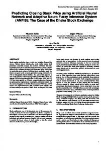
0.05 0.045 0.04

HVIX

0.035 0.03

30 25 20 0

50

100

150

200

0.025

300

350

400

450

12-day EMA 26-day EMA

0.015 0.01 0.005 0

50

100 150 200 250 300 350 400 450 500 date

HVIX12 HVIX26

Figure 1: Historical volatility of “-zgrs-” with the buy-and-sell strategy.

3, 2017, from the Shanghai stock market to test a 5 d buyand-hold strategy and use the historical data for the stock “payh-” from June 22, 1993, to May 10, 2010, from the Shanghai stock market to test a 10 d buy-and-hold strategy. The detailed trading strategy is similar to the buy-and-sell strategy. Here, we use m = 12, n = 26, and p = 9.

5. Empirical Results 5.1. Empirical Results of Buy-and-Sell Strategy. From the “zgrs-” stock data chosen in Section 4, we calculate the HVIX of the past m days and the past n days. A higher stock index means that investors feel anxiety regarding the stock market, and a lower stock index means that the rate of change of the stock price will decrease. Figure 1 shows the HVIX index. Next, using the calculated volatility index, we calculate the weight of the EMA formula in Section 3 and obtain the values of MACD-HVIX, DEA-HVIX, and OSC. Figure 2 shows the candlestick chart and MACD histogram. In the candlestick chart, the blue line represents the 12-d EMA, and the red line represents the 26-d EMA. Candlesticks are usually composed of a red and green body, as well as an upper wick and a lower wick. The area between the opening and the closing prices is called the body, and price excursions above or below the real body are called the wick. The body indicates the opening and closing prices, and the wick indicates the highest and lowest traded prices of a stock during the time interval represented. For a red body, the opening price is at the bottom, and the closing price is at the top. For a green body, the opening price is at the top, and the closing price is at the bottom. In the MACD histogram, the solid line represents the DIF, the dotted line represents the DEA, and the histogram represents the MACD bar. According to the strategy described in Section 3, we buy the stock when the DIF and DEA are positive, the DIF cuts the DEA in an uptrend, and the

MACD histogram

0.02

0

250 date

1 0 −1 −2

Sell

0

50

100

DIF DEA MACD bar

150

Buy

200

250 date

Buy Buy

300

Sell Buy Buy

350

400

450

Figure 2: Candlestick chart and MACD histogram for “-zgrs-” with the buy-and-sell strategy. (For interpretation of the references to color in the figure, the reader is referred to the web version of the article.)

divergence is positive. We sell the stock when the DEA cuts the DIF in a downtrend, and the divergence is negative. As shown in Figure 2, we sell the stock on days 155 and 355 and buy the stock on days 212, 290, 310, 381, and 393. The buy-andsell signals in the candlestick chart and the MACD histogram are shown in Figure 3. Figure 4 shows the candlestick chart and MACD histogram of HVIX. In the candlestick chart, the blue line represents the 12-d EMA-HVIX, and the red line represents the 26-d EMA-HVIX. In the MACD-HVIX histogram, the solid line represents the DIF-HVIX, the dotted line represents the DEA-HVIX, and the histogram represents the MACDHVIX bar. According to the strategy described in Section 3, we buy the stock when the DIF-HVIX and DEA-HVIX are positive, the DIF-HVIX cuts the DEA-HVIX in an uptrend, and the divergence is positive, and we sell the stock when the DEA-HVIX cuts the DIF-HVIX in a downtrend, and the divergence is negative. As shown in Figure 4, we sell the stock on days 118 and 187 and buy the stock on days 222, 231, 241, 243, 292, 415, and 447. The buy-and-sell signals in the candlestick chart and the MACD histogram are shown in Figure 5. To verify the stability of the new indicator, we compare the MACD and MACD-HVIX in Figure 6. The MACD and MACD-HVIX have basically the same trend and the stability of the MACD-HVIX is better than that of the MACD. Table 1 shows a comparison of the specific values of the buying-selling points for the MACD index and MACDHVIX index, as well as a comparison of the predicted and actual trends. Here, we see that the prediction accuracy of MACD-HVIX is 0.667 and that of MACD is 0.4286. By using the proposed indicator, we can improve the prediction accuracy by 55.55% compared with the traditional MACD. The “-Price-” in the table represents the closing price of


5 23 Candlestick chart

Candlestick chart

23 22 21 20 19 140

145

150

155 date

165

200

Sell 150

DIF

155 date

160

165

−2

Buy 200

210 212 215 date

205

DIF Candlestick chart

Candlestick chart

225

−1

170

26 24

280

285

290 295 date 26-day EMA

12-day EMA

300

DEA

220

225

MACD bar

MACD histogram

0

Buy 280

285

DIF

290 date

295

DEA

24

300

305

310 date

300

305

315

320

325

320

325

26-day EMA

12-day EMA

−1 −2 275

26

22 295

305

1

MACD histogram

215 220 date 26-day EMA

28

22 275

1 0 −1 −2 295

MACD bar

Buy 300

305

DIF

310 date

315

DEA

MACD bar

30 Candlestick chart

28 26 24 22 340

345

350

355 date

360

365

24 370

0 −1 Sell 350

DIF

355 date

360

DEA

375

380 date

365

370

390

395

390

395

1 0 −1 −2

Buy 370 DIF

MACD bar

385

26-day EMA

12-day EMA

1

345

26

26-day EMA

12-day EMA

−2 340

28

370

MACD histogram

Candlestick chart

210

0

MACD bar

DEA

205

1

MACD histogram

−1

28

MACD histogram

19

12-day EMA

0

145

20

170

1

−2 140

21

26-day EMA

12-day EMA MACD histogram

160

22

380 381 date

375 DEA

385

MACD bar

Candlestick chart

30 28 26 24 380

385

390

395

400

405

date 26-day EMA

MACD histogram

12-day EMA 1 0 −1 −2

Buy 380

385 DIF

390 DEA

393 395 date

400

405

MACD bar

Figure 3: Buy-and-sell signals in the candlestick chart and MACD histogram for the buy-and-sell strategy.

6

Mathematical Problems in Engineering Table 1: Comparison of the specific values of the buying-selling points for the buy-and-sell strategy.

MACD

Test date 155 212 290 310 355 381 393

Price (Test date) 20.39 21.82 25.32 26.44 24.51 27.93 29.00

118 187 222 231 241 243 292 415 447

22.24 20.80 21.90 21.80 21.65 21.78 25.18 27.98 29.27

Price (Test date + 1 d) 20.42 21.93 25.38 26.50 24.62 27.45 28.48 0.4286 21.90 20.66 21.84 21.67 21.58 21.83 25.58 28.80 29.51 0.6667

Win rate

MACD-HVIX

Candlestick chart

Win rate

30 25 20 0

50

100

150

200

250 date

300

350

400

450

MACD-HVIX histogram

12-day EMA-HVIX 26-day EMA-HVIX 1 0 −1 Sell

Sell

−2 0

50

100

150

Buy Buy Buy Buy

200

250 date

Buy

300

Buy

350

400

Buy

450

DIF-HVIX DEA-HVIX MACD-HVIX bar

Figure 4: Candlestick chart and MACD-HVIX histogram for “zgrs-” with the buy-and-sell strategy. (For interpretation of the references to color in this figure, the reader is referred to the web version of the article.)

stock. Next, we compare the cumulative returns for the two indicators. According to the trading points shown in the table, we perform a simulation test. We assume that the initial fund is 1 million. The cumulative returns under the two indexes are 1.1136 million and 1.3365 million, for MACD and MACDHVIX indices, respectively.

Predicted trend ↓ ↑ ↑ ↑ ↓ ↑ ↑

Actual trend ↑ ↑ ↑ ↑ ↑ ↓ ↓

↓ ↓ ↑ ↑ ↑ ↑ ↑ ↑ ↑

↓ ↓ ↓ ↓ ↓ ↑ ↑ ↑ ↑

5.2. Empirical Results of Buy-and-Hold Strategy. Using the “dggf-” stock data chosen in Section 4, we first investigate the buy or sell points for both the indicators with the buy-andhold strategy applied for 5 d. Then, we compare the prediction accuracy between the two indicators. The MACD histogram shown in Figure 7 indicates the buy-and-sell points; we should buy the stock at a buy point on days 391, 1,071, 1,181, 1,326, and 1,481, and sell the stock at a sell point on days 791, 881, and 911. The prediction situation is shown in Table 2. The MACD-HVIX histogram in Figure 8 indicates the buy-and-sell points. We should buy the stock at a buy point on days 371, 1,201, 1,331, and 1,561 and sell the stock at a sell point on days 751 and 771. The prediction situation is shown in Table 2. A comparison between MACD and MACD-HVIX is shown in Figure 9. Table 2 shows a comparison of the specific values of the buying-selling points for the MACD and MACD-HVIX indices with the buy-and-hold strategy for 5 d, as well as a comparison of the predicted and actual trends. Here, we observe that the prediction accuracy of MACD-HVIX is 0.8333 and that of MACD is 0.6250. By using the proposed indicator, we can improve the prediction accuracy by 33.33% compared with the traditional MACD. The “-Price-” in the table represents the closing price of the stock. Next, using the “-payh-” stock data chosen in Section 4, we investigate the buy or sell points for both the indicators with the buy-and-hold strategy applied for 10d. Then, we compare the prediction accuracy between the two indicators. The MACD histogram in Figure 10 indicates the buy-and-sell points. We should buy the stock at a buy point on day 901, and sell the stock at a sell point on days 621, 1,971, 2,071, 2,291, 2,431, and 2,661. The prediction situation is shown in Table 3. The MACD-HVIX histogram in Figure 11 indicates the buy-and-sell points. We should buy the stock at a buy point


7


Candlestick chart

24 22 20 18 105

110

115

120

125

22 20 18 175

130

180

185

1 0 −1 Sell

−2 110

195

200

190

195

200

12-day EMA-HVIX 26-day EMA-HVIX MACD-HVIX histogram

MACD-HVIX histogram

12-day EMA-HVIX 26-day EMA-HVIX

105

190 date

date

118 120 date

115

125

1 0 −1 Sell

−2 175

130

180

185 187 date




Candlestick chart

24 22 20

22 20 18

18

220 210

215

220

225

230

225

230 date

235

date

MACD-HVIX histogram

MACD-HVIX histogram

1 0 −1 Buy 210

215

220 222 date

225

230

235

240

245

0 −1 Buy

−2 220

230 231 date

225

235 DIF-HVIX DEA-HVIX MACD-HVIX bar

24


Candlestick chart

245

1


22 20 18 230

235

240

245

250

22 20 18

255

230

235

240

MACD-HVIX histogram

1 0 −1 Buy 230

235

250

255

243 245 date

250

255



−2

245 date

date

MACD-HVIX histogram

240



−2

235

240 241 date

245

250

1 0 −1 Buy

−2

255

230

235



Figure 5: Continued.

240

8

Mathematical Problems in Engineering 28 Candlestick chart

Candlestick chart

30 26 24 22 20

280

285

290

295

300

28 26 24 22 400

305

405

410

date

1 0 −1 Buy 280

285

420

425

430

420

425

430

12-day EMA-HVIX 26-day EMA-HVIX MACD-HVIX histogram

MACD-HVIX histogram


−2

415 date

290 292 date

295

300

1 0 −1 Buy

−2 400

305


405

410

415 date


Candlestick chart

30 28 26 24 22

435

440

445

450

455

460

450

455

460

date

MACD-HVIX histogram

12-day EMA-HVIX 26-day EMA-HVIX 1 0 −1 Buy

−2 435

440

445 447 date


Figure 5: Buy-and-sell signals in the candlestick chart and the MACD-HVIX histogram for the buy-and-sell strategy.

on day 901 and sell the stock at a sell point on days 2,071, 2,421, 2,661, and 2,741. The prediction situation is shown in Table 3. A comparison of MACD and MACD-HVIX is presented in Figure 12. Table 3 shows the comparison of the specific values of the buying-selling points for the MACD and MACD-HVIX indices with the buy-and-hold strategy applied for 5 d, as well as a comparison of the predicted and actual trends. Here, we observe that the prediction accuracy of MACD-HVIX is 0.8 and that of MACD is 0.7143. By using the proposed indicator, we can improve the prediction accuracy by 12% compared with the traditional MACD. The “-Price-” in the table represents the closing price of the stock. 5.3. Computational Complexity. The computational complexity of the MACD and MACD-HVIX for a stock which

has a length of n are 𝑂(𝑁) and 𝑂(𝑁2 ), respectively. In terms of trend prediction processing time, the average time required to process a buy-and-sell strategy, a buy-and-hold strategy for 5 days, and a buy-and-hold strategy for 10 days with the MACD approach (MACD-HVIX) are, respectively, 1.25 (1.51), 1.12 (1.35), and 1.41 seconds (1.58) using Matlab R2017b on an Intel(R) Core(TM) i5-6200 CPU @ 2.30GHz processor.

6. Conclusion As indicated by Tables 1, 2, and 3, we buy-and-sell stock based on improved MACD; then we found all the accuracy is higher than that before the improvement. Therefore, the improved model has higher maneuverability in securities investment and allows investors to capture every buy-and-sell points in


9

Table 2: Comparison of the specific values of the buying-selling points with the buy-and-hold strategy applied for 5 d.

MACD

Test date 391 791 881 911 1071 1181 1326 1481

Price (Test date) 13.04 4.81 5.55 5.71 6.57 6.66 10.70 17.28

371 751 771 1201 1331 1561

11.68 5.53 5.76 7.66 11.93 16.89

Win rate

MACD-HVIX

Win rate

Candlestick chart

0.4 0.2

Predicted trend ↑ ↓ ↓ ↓ ↑ ↑ ↑ ↑

Actual trend ↑ ↑ ↑ ↓ ↑ ↑ ↑ ↓

↑ ↓ ↓ ↑ ↑ ↑

↑ ↑ ↓ ↑ ↑ ↑

20 10 0

0

200

400

600

0

800 1000 1200 1400 1600 1800 date

12-day EMA 26-day EMA −0.2 −0.4 −0.6

0

50

100 150 200 250 300 350 400 450 500 date

MACD bar MACD-HVIX bar

Figure 6: Comparison of the two indicators for the buy-and-sell strategy.

the market. For both the buy-and-sell strategy and the buyand-hold strategy, the empirical results indicated that the proposed model can make more precise predictions than the traditional model. The proposed model was tested with three different stocks and it generated the high prediction accuracy for all the cases. In addition, while a smoothing index is used to construct the MACD index and the impact of the past price declines exponentially, the MACD-HVIX does not have this property. Although the MACD-HVIX index is improved compared with the MACD index, the stationarity of the MACD-HVIX index is difficult prove theoretically. Test shows that it is stable; however, in the ever-changing market, an abnormal situation can cause incalculable losses to

MACD histogram

MACD bar and MACD-HVIX bar

0.6

Price (Test date + 5 d) 15.70 5.19 5.61 5.59 6.74 6.95 11.93 13.51 0.6250 12.00 5.75 5.62 7.83 12.23 19.05 0.8333

4 2 0 −2

Sell Sell Sell

Buy

0

200

400

DIF DEA MACD bar

600

Buy Buy

Buy

Buy

800 1000 1200 1400 1600 1800 date

Figure 7: Candlestick chart and MACD histogram for “-dggf-” with the buy-and-hold strategy applied for 5 d. (For interpretation of the references to color in this figure, the reader is referred to the web version of the article.)

investors. In future research, we will investigate other factors for the model by constantly updating the data and the training model to obtain a better prediction effect.

Data Availability The data used to support the findings of this study are available from the corresponding author upon request.

10

Mathematical Problems in Engineering Table 3: Comparison of the specific values of the buying-selling points with the buy-and-hold strategy applied for 10 d.

MACD

Test date 621 901 1971 2071 2291 2431 2661

Price (Test date) 6.59 18.87 13.05 12.25 11.11 10.56 8.51

901 2071 2421 2661 2741

18.87 12.25 11.30 8.51 6.95

Price (Test date + 10 d) 6.23 19.05 13.22 10.31 10.52 10.81 8.23 0.7143 19.05 10.31 10.56 8.23 7.19 0.8000

Win rate

MACD-HVIX

Candlestick chart

Win rate

Actual trend ↓ ↑ ↑ ↓ ↓ ↑ ↓

↑ ↓ ↓ ↓ ↓

↑ ↓ ↓ ↓ ↑

20 10 0

MACD-HVIX histogram

Predicted trend ↓ ↑ ↓ ↓ ↓ ↓ ↓

0

200

400

0

200

400

600

800 1000 1200 1400 1600 1800 date 12-day EMA-HVIX 26-day EMA-HVIX

4 2 0 −2

Buy

Sell Sell

600

Buy Buy

Buy

800 1000 1200 1400 1600 1800 date


Figure 8: Candlestick chart and MACD-HVIX histogram for “-dggf-” with the buy-and-hold strategy for 5 d. (For interpretation of the references to color in this figure, the reader is referred to the web version of the article.)


1.5 1 0.5 0 −0.5 −1 −1.5

0

200 400 600 800 1000 1200 1400 1600 1800 2000 date MACD bar MACD-HVIX bar

Figure 9: Comparison of the two indicators with the buy-and-hold strategy applied for 5 d.

11 3

40 20 0

0

500

1000

1500

2000 date

2500

3000

3500

4000

MACD histogram

12-day EMA 26-day EMA 10 5 0 −5

Se ll Buy

0

500

1000

2000 date

2500

3000

3500

Candlestick chart MACD-HVIX histogram

0 −1 −2

0

500

1000 1500 2000 2500 3000 3500 4000 4500 date

MACD bar MACD-HVIX bar

Figure 10: Candlestick chart and MACD histogram for “-payh-” with the buy-and-hold strategy applied for 10 d. (For interpretation of the references to color in this figure, the reader is referred to the web version of the article.)

Figure 12: Comparison of the two indicators with the buy-and-hold strategy applied for 10 d.

author (J.S. Kim) expresses thanks for the support from the BK21 PLUS program.

References

40 20 0

500

1000

1500

2000 date

2500

3000

3500

4000

3000

3500

4000

12-day EMA-HVIX 26-day EMA-HVIX 10 5 0 −5

1

4000

DIF DEA MACD bar

0

2

−3

Sell Sell Sell Sell Sell

1500


Candlestick chart


Buy

0

500

1000

Sell

1500

2000 date

Sell Sell Sell

2500


Figure 11: Candlestick chart and MACD-HVIX histogram for “-payh-” with the buy-and-hold strategy applied for 10 d. (For interpretation of the references to color in this figure, the reader is referred to the web version of the article.)

Conflicts of Interest The authors declare that there are no conflicts of interest regarding the publication of this paper.

Acknowledgments The first author (Jian Wang) was supported by the China Scholarship Council (201808260026). The corresponding

[1] F. Schmitt, D. Schertzer, and S. Lovejoy, “Multifractal Fluctuations in Finance,” International Journal of Theoretical and Applied Finance, vol. 03, no. 03, pp. 361–364, 2000. [2] T. J. Moskowitz, Y. H. Ooi, and L. H. Pedersen, “Time series momentum,” Journal of Financial Economics, vol. 104, no. 2, pp. 228–250, 2012. [3] C. S. Asness, T. J. Moskowitz, and L. H. Pedersen, “Value and Momentum Everywhere,” Journal of Finance, vol. 68, no. 3, pp. 929–985, 2013. [4] M. R. Hassan, “A combination of hidden Markov model and fuzzy model for stock market forecasting,” Neurocomputing, vol. 72, no. 16-18, pp. 3439–3446, 2009. [5] P. Pai, L. Hong, and K. Lin, “Using Internet Search Trends and Historical Trading Data for Predicting Stock Markets by the Least Squares Support Vector Regression Model,” Computational Intelligence and Neuroscience, vol. 2018, Article ID 6305246, 15 pages, 2018. [6] S. Lahmiri, “Minute-ahead stock price forecasting based on singular spectrum analysis and support vector regression,” Applied Mathematics and Computation, vol. 320, pp. 444–451, 2018. [7] P. Singh and B. Borah, “Forecasting stock index price based on M-factors fuzzy time series and particle swarm optimization,” International Journal of Approximate Reasoning, vol. 55, no. 3, pp. 812–833, 2014. [8] S. Lahmiri and M. Boukadoum, “Intelligent Ensemble Forecasting System of Stock Market Fluctuations Based on Symetric and Asymetric Wavelet Functions,” Fluctuation and Noise Letters, vol. 14, no. 4, 2015. [9] S. R. Das, D. Mishra, and M. Rout, “A hybridized ELM using self-adaptive multi-population-based Jaya algorithm for currency exchange prediction: an empirical assessment,” Neural Computing and Applications, pp. 1–24, 2018.

12 [10] L. A. Laboissiere, R. A. S. Fernandes, and G. G. Lage, “Maximum and minimum stock price forecasting of Brazilian power distribution companies based on artificial neural networks,” Applied Soft Computing, vol. 35, pp. 66–74, 2015. [11] L. Lei, “Wavelet Neural Network Prediction Method of Stock Price Trend Based on Rough Set Attribute Reduction,” Applied Soft Computing, vol. 62, pp. 923–932, 2018. [12] S. Lahmiri, “Intraday stock price forecasting based on variational mode decomposition,” Journal of Computational Science, vol. 12, pp. 23–27, 2016. [13] S. Lahmiri, “A Technical Analysis Information Fusion Approach for Stock Price Analysis and Modeling,” Fluctuation and Noise Letters, vol. 17, no. 01, p. 1850007, 2018. [14] J.-Z. Wang, J.-J. Wang, Z.-G. Zhang, and S.-P. Guo, “Forecasting stock indices with back propagation neural network,” Expert Systems with Applications, vol. 38, no. 11, pp. 14346–14355, 2011. [15] Y. Shynkevich, T. M. McGinnity, S. A. Coleman, A. Belatreche, and Y. Li, “Forecasting price movements using technical indicators: Investigating the impact of varying input window length,” Neurocomputing, vol. 264, pp. 71–88, 2017. ˇ [16] I. Svalina, V. Galzina, R. Luji´c, and G. Simunovi´ c, “An adaptive network-based fuzzy inference system (ANFIS) for the forecasting: the case of close price indices,” Expert Systems with Applications, vol. 40, no. 15, pp. 6055–6063, 2013. [17] X. Zhou, Z. Pan, G. Hu, S. Tang, and C. Zhao, “Stock Market Prediction on High-Frequency Data Using Generative Adversarial Nets,” Mathematical Problems in Engineering, vol. 2018, Article ID 4907423, 11 pages, 2018. [18] Z. Wang, J. Hu, and Y. Wu, “A Bimodel Algorithm with DataDivider to Predict Stock Index,” Mathematical Problems in Engineering, vol. 2018, Article ID 3967525, 14 pages, 2018. [19] S. Lahmiri, “Interest rate next-day variation prediction based on hybrid feedforward neural network, particle swarm optimization, and multiresolution techniques,” Physica A: Statistical Mechanics and its Applications, vol. 444, pp. 388–396, 2016. [20] L. Tao, Y. Hao, H. Yijie, and S. Chunfeng, “K-Line Patterns’ Predictive Power Analysis Using the Methods of Similarity Match and Clustering,” Mathematical Problems in Engineering, vol. 2017, Article ID 3096917, 11 pages, 2017.


Advances in

Operations Research Hindawi www.hindawi.com

Volume 2018

Advances in

Decision Sciences Hindawi www.hindawi.com

Volume 2018

Journal of

Applied Mathematics Hindawi www.hindawi.com

Volume 2018

The Scientific World Journal Hindawi Publishing Corporation http://www.hindawi.com www.hindawi.com

Volume 2018 2013

Journal of

Probability and Statistics Hindawi www.hindawi.com

Volume 2018

International Journal of Mathematics and Mathematical Sciences

Journal of

Optimization Hindawi www.hindawi.com

Hindawi www.hindawi.com

Volume 2018

Volume 2018

Submit your manuscripts at www.hindawi.com International Journal of

Engineering Mathematics Hindawi www.hindawi.com

International Journal of

Analysis

Journal of

Complex Analysis Hindawi www.hindawi.com

Volume 2018


Stochastic Analysis Hindawi www.hindawi.com


Volume 2018

Volume 2018

Advances in

Numerical Analysis Hindawi www.hindawi.com

Volume 2018

Journal of


Volume 2018

Journal of

Mathematics Hindawi www.hindawi.com


Function Spaces Volume 2018


Volume 2018


Differential Equations Hindawi www.hindawi.com

Volume 2018

Abstract and Applied Analysis Hindawi www.hindawi.com

Volume 2018

Discrete Dynamics in Nature and Society Hindawi www.hindawi.com

Volume 2018

Advances in

Mathematical Physics Volume 2018


Volume 2018