Pricing and Flow Control in Communications Networks by ... - CiteSeerX

Pricing and Flow Control in Communications Networks by John T. Musacchio

B.S. (The Ohio State University) 1996 M.S. (The University of California, Berkeley) 1998

A dissertation submitted in partial satisfaction of the requirements for the degree of Doctor of Philosophy in Engineering - Electrical Engineering and Computer Sciences in the GRADUATE DIVISION of the UNIVERSITY of CALIFORNIA, BERKELEY

Committee in charge: Professor Jean Walrand, Chair Professor Pravin Varaiya Professor John Chuang Spring 2005

The dissertation of John T. Musacchio is approved:

Chair

Date

Date

Date

University of California, Berkeley

Spring 2005

Pricing and Flow Control in Communications Networks

Copyright 2005 by John T. Musacchio

1

Abstract

Pricing and Flow Control in Communications Networks by John T. Musacchio Doctor of Philosophy in Engineering - Electrical Engineering and Computer Sciences University of California, Berkeley Professor Jean Walrand, Chair

In the first part of this dissertation, we study the economic interests of a wireless access point owner and his paying client, and model their interaction as a dynamic game. The key feature of this game is that the players have asymmetric information – the client knows more than the access provider. We find that if a client has a “web browser” utility function (a temporal utility function that grows linearly), it is a Nash equilibrium for the provider to charge the client a constant price per unit time. On the other hand, if the client has a “file transferor” utility function (a utility function that is a step function), the client would be unwilling to pay until the final time slot of the file transfer. We also study an expanded game where an access point sells to a reseller, which in turn sells to a mobile client and show that if the client has a web browser utility function, that constant price is a Nash equilibrium of the three player game. Finally, we study a two player game in which the access point does not know whether he faces a web browser or

2 file transferor type client, and show conditions for which it is not a Nash equilibrium for the access point to maintain a constant price. In the second part of this dissertation we study a simple ingress policing scheme for a stochastic queuing network that uses a round-robin service discipline, and derive conditions under which the flow rates approach a max-min fair share allocation. The scheme works as follows: Whenever any of a flow’s queues exceeds a policing threshold, the network discards that flow’s arriving packets at the network ingress, and does so until all of that flow’s queues fall below their thresholds. To prove our results, we consider the fluid limit of a sequence of queuing networks with increasing thresholds. Using a Lyapunov function derived from the fluid limits, we find that as the policing thresholds are increased, the state of the stochastic system is attracted to a smaller and smaller neighborhood surrounding the equilibrium of the fluid model. We then show how this property implies that the achieved flow rates approach the max-min rates predicted by the fluid model.

Professor Jean Walrand Dissertation Committee Chair

i

To my mother and father.

ii

Contents List of Figures

v

I

1

WiFi Pricing

1 Introduction 1.1 Alternative Charging Models . . . . . 1.2 Making the P2P Model Viable . . . . 1.3 The Problem of Contract Enforcement 1.4 Possible Payment Architecture . . . . 1.5 Security Issues . . . . . . . . . . . . . 1.6 Previous Work . . . . . . . . . . . . . 1.7 Overview . . . . . . . . . . . . . . . .

. . . . . . .

. . . . . . .

. . . . . . .

. . . . . . .

. . . . . . .

2 . 3 . 4 . 5 . 5 . 7 . 8 . 10

2 Game-Theoretic Analysis 2.1 Basic Model . . . . . . . . . . . . . . . . . . . . . . . . . . . . . . 2.2 Web Browsing Model . . . . . . . . . . . . . . . . . . . . . . . . . 2.2.1 Web Browsing Examples . . . . . . . . . . . . . . . . . . . 2.2.2 Uniqueness of the PBE . . . . . . . . . . . . . . . . . . . 2.2.3 Multiple Hops . . . . . . . . . . . . . . . . . . . . . . . . 2.3 File Transfer Model . . . . . . . . . . . . . . . . . . . . . . . . . 2.3.1 Inefficiency of the File Transfer Model Equilibrium . . . . 2.4 Bayesian Model . . . . . . . . . . . . . . . . . . . . . . . . . . . . 2.4.1 Unbounded Length . . . . . . . . . . . . . . . . . . . . . . 2.5 Result Summary and Implications to P2P Model of WiFi Pricing

. . . . . . . . . .

. . . . . . . . . .

. . . . . . . . . .

. . . . . . . . . .

. . . . . . . . . .

. . . . . . . . . . . . . . . . . . . . in a P2P Model . . . . . . . . . . . . . . . . . . . . . . . . . . . . . . . . . . . . . . . . .

. . . . . . .

. . . . . . .

. . . . . . .

. . . . . . .

11 11 13 17 18 19 27 30 31 37 40

3 Dynamic Programming Formulation of Returning Clients 43 3.1 Model . . . . . . . . . . . . . . . . . . . . . . . . . . . . . . . . . . . . . . 44 3.2 Results . . . . . . . . . . . . . . . . . . . . . . . . . . . . . . . . . . . . . . 46 3.3 Concluding Remarks . . . . . . . . . . . . . . . . . . . . . . . . . . . . . . 52

iii

II

Achieving Fair Rates with Ingress Policing

54

4 Introduction 55 4.1 Motivation . . . . . . . . . . . . . . . . . . . . . . . . . . . . . . . . . . . 56 4.2 Related Work . . . . . . . . . . . . . . . . . . . . . . . . . . . . . . . . . . 62 5 Model 5.1 Flows and Classes . . . . . . . . . . . . . . . . . . . . . 5.2 Queues . . . . . . . . . . . . . . . . . . . . . . . . . . . . 5.3 Policing Points . . . . . . . . . . . . . . . . . . . . . . . 5.4 A Simple Example . . . . . . . . . . . . . . . . . . . . . 5.5 Threshold Scaling . . . . . . . . . . . . . . . . . . . . . . 5.6 Candidate Equilibrium and “Relative” Initial Condition 5.7 Dynamics of System-n . . . . . . . . . . . . . . . . . . . 5.7.1 Arrivals, Departures, and Routing . . . . . . . . 5.7.2 Queueing Discipline . . . . . . . . . . . . . . . . 5.7.3 Trajectory Notation . . . . . . . . . . . . . . . .

. . . . . . . . . .

. . . . . . . . . .

. . . . . . . . . .

. . . . . . . . . .

. . . . . . . . . .

. . . . . . . . . .

. . . . . . . . . .

. . . . . . . . . .

. . . . . . . . . .

. . . . . . . . . .

66 66 67 68 69 73 74 75 76 77 78

6 Proof Strategy 80 6.1 Result Summary . . . . . . . . . . . . . . . . . . . . . . . . . . . . . . . . 83 7 Fluid Limit Analysis 7.1 Preliminary Lemmas . . . . . . . . . . . . . . . . . . . . . . . . . . . . . . 7.2 Convergence to a Fluid Limit along a Subsequence . . . . . . . . . . . . . 7.2.1 Sliding Modes . . . . . . . . . . . . . . . . . . . . . . . . . . . . . . 7.3 Upgrading Convergence along Subsequences to Convergence on Sequences 7.4 Convergence to Fluid Model Rates on a Compact Time Interval . . . . . . 7.5 Stochastic System Attracted to Fluid Equilibrium . . . . . . . . . . . . . 7.6 Hitting Times on a Neighborhood of the Fluid Equilibrium . . . . . . . . 7.7 Convergence of Long Term Rates . . . . . . . . . . . . . . . . . . . . . . . 8 Round Robin Network without Loops 8.1 Fluid Model Example. . . . . . . . . . . . . . . . . . . . . . 8.2 Pipeline Notation and Properties . . . . . . . . . . . . . . . 8.3 Max-Min Fair Definitions . . . . . . . . . . . . . . . . . . . 8.4 Fluid Model Rate Lemmas . . . . . . . . . . . . . . . . . . . 8.5 Demand Limited Flow Analysis . . . . . . . . . . . . . . . . 8.6 Bottleneck Limited Flow Analysis . . . . . . . . . . . . . . . 8.7 Final Result . . . . . . . . . . . . . . . . . . . . . . . . . . . 8.8 Relaxing the Unique Bottleneck Requirement . . . . . . . . 8.9 Uniformity of the Required Threshold for Different Demand 9 Conclusion

. . . . . . . . . . . . . . . . . . . . . . . . . . . . . . . . . . . . . . . . . . . . . . . . Processes

. . . . . . . . .

86 86 91 98 100 102 104 107 111

119 . 120 . 125 . 128 . 130 . 131 . 134 . 146 . 149 . 150 152

iv A

154 A.1 Further Explanation of Proof of Theorem 7.10 . . . . . . . . . . . . . . . . 154 A.2 Proofs of Lemmas in Chapter 8 . . . . . . . . . . . . . . . . . . . . . . . . 155

Bibliography

162

v

List of Figures 1.1

Payment architecture. . . . . . . . . . . . . . . . . . . . . . . . . . . . . .

2.1 2.2

Multi-hop scenario . . . . . . . . . . . . . . . . . . . . . . . . . . . . . . . 19 PBE prices in Bayesian game. . . . . . . . . . . . . . . . . . . . . . . . . . 32

3.1 3.2 3.3 3.4 3.5

Optimal Optimal Optimal Optimal Optimal

4.1

A two input, two output switch with virtual output queues. . . . . . . . . 57

5.1

Trajectories of an example network. . . . . . . . . . . . . . . . . . . . . . 70

7.1

The stopping times σi , σi+1 , ... and the expected throughput. . . . . . . . 114

8.1 8.2 8.3 8.4 8.5

Fluid model trajectory for the example network. Flow pipeline and available rates. . . . . . . . . . The analysis of downstream queues. . . . . . . . Upstream queue Lyapunov function level set. . . Upstream queue analysis. . . . . . . . . . . . . .

reward to go for α = 0.7. . . . . . . . . . . . . price as a function of lower bound, for α = 0.7 price decision tree for α = 0.7 . . . . . . . . . . price as a function of lower bound, for α = 0.99 price for α = 0.5, 0.7, 0.9, 0.99 . . . . . . . . .

. . . . .

. . . . .

. . . . .

. . . . .

. . . . .

. . . . .

. . . . .

. . . . .

. . . . .

. . . . .

. . . . .

. . . . .

. . . . .

. . . . .

. . . . .

. . . . .

. . . . .

. . . . .

. . . . .

. . . . .

. . . . .

. . . . .

. . . . .

. . . . .

6

47 48 50 51 52

120 137 138 142 142

vi

Acknowledgements First and foremost, I would like to thank my advisor Jean Walrand. Without his guidance and support, this dissertation would not have been possible. I am indebted to him not only for what he has taught me technically, but also for all of the other insight that he has shared with me over the years that I know will benefit me in many ways throughout my career. I am especially grateful for his patience and advice when progress was difficult. I also thank my other dissertation committee members, Pravin Varaiya and John Chuang, for their helpful advice and for the interest and enthusiasm they have shown for my work. Thanks also go to Kameshwar Poolla, who served on my qualifying committee and to Costas Spanos who with Kameshwar Poolla co-advised my master’s degree studies. Their guidance and patience was invaluable to me during my first two years of graduate study at Berkeley. I also thank the Berkeley graduate students, as well as the former students of my advisor, with whom I have worked with over the years. They include: Gaurav Agrawal, Antonis Dimakis, Rajarshi Gupta, Linhai He, Jeonghoon Mo, Shyam Parekh and Teresa Tung. I enjoyed working with and learned a lot from each of them. This work was supported by the Defense Advanced Research Project Agency under Grant N66001-00-C-8062 and by the National Science Foundation under grant ANI-0331659. During my years of graduate study at Berkeley, I was also supported by a Department of Defense National Defence Science and Engineering Graduate Fellowship, and a Fellowship from the California State MICRO Program.

vii

Preface This dissertation addresses two important problems in communications networks. Part I addresses the problem of WiFi access point pricing by modelling the interaction of an access point owner and paying client as a dynamic game. Part II addresses the problem of flow control in a queueing network. In particular, we show that a simple ingress policing scheme is capable of achieving long-term average flow rates that are arbitrarily close to being max-min fair. To prove our result, we show that the flow rates of the stochastic network approach the flow rates of a fluid model.

1

Part I

WiFi Pricing

2

Chapter 1

Introduction Today there is a large and growing number of wireless access points deployed by homes and businesses for private LANs. Many of these access points could potentially be used to provide Internet access to users from the general public that lie or are passing within communication range of the access point. However, owners of private WiFi networks often choose to encrypt their networks to prevent outsiders from accessing them. Without a mechanism for a potential client to compensate the owner of the network, the network owner has no reason to accept the increased network traffic and security risk that would come from allowing the public to access his network. If it were possible to incentivize owners of existing private wireless access points to open their networks to the public, as well as incentivize people and institutions to deploy access points where there are gaps in coverage, the result might be nearly ubiquitous WiFi coverage. In contrast to cellular phone networks deployed by a few large providers, this ubiquitous access network would be deployed by thousands, perhaps millions, of

3 autonomous self-interested agents.

1.1

Alternative Charging Models

The simplest way for a client to compensate an access point owner would be for the client to just pay the access point directly. We refer to this as the Peer to Peer (P2P) model, because it does not involve a 3rd party. Other models are possible. One model that is becoming increasingly popular is the aggregator model. In the model, the deploying business partners with an aggregator franchise, such as Boingo [19]. The aggregator attaches its brand name to hot spots and ensures that a consistent product is offered among the hot spots deployed by different businesses. The aggregator also handles the billing for the service, and can offer the user subscription billing plans that apply to all of the branded hot spots. The aggregator collects the revenue from the client, and then redistributes some of the revenue to the deploying business partners. This model will likely continue to grow in popularity, but because it requires a third party to monitor that each access point adhere to the standards of the aggregator brand name, it is not clear whether this model could scale to millions of access points. Perhaps, an aggregator model more like that used by online auction sites would be more scalable; a model in which clients can view a reputation rating based on past clients feedback, but where the aggregator does not guarantee the trustworthiness of a particular access point. In this work we will not study the aggregator model further, but instead we will focus on studying the properties and viability of a P2P model involving the two principle parties, access point and client, with minimal or no third party involvement.

4

1.2

Making the P2P Model Viable

Though the P2P model has the potential of being more scalable than the aggregator model, there are a number of challenges in making a P2P model viable. In many cases a client and access point may not know each other’s identity, and may not be able to trust each other to carry out their side of a transaction. To understand the problem, imagine a scheme where the client pays for her entire session in one lump payment. In a scheme where the client pays the access point in advance, or pre-pay scheme, a malicious access point might accept payment and then fail to deliver service. In a post-pay scheme, a client may fail to make a promised payment after receiving service. In fact, if we imagine that the access point and client are players in a game, and are trying to maximize their reward from this single transaction, a client should try to obtain service without paying, and a access point should try to take the client’s money without giving him any service. Therefore, we must take care in structuring the game in a way that deters the players from cheating. Yet at the same time, we would like to avoid introducing a third party enforcement agent to the game. In an implementation, an enforcement agent would probably have to be centralized, and thus might limit scalability. One possibility would be for the client to pay the access point in small amounts over the duration of the session. The intuition justifying this scheme is that a access point will want to play “fair”, lest it be punished by being denied payments in the future, and a client will want to keep paying throughout the session to ensure that its service is not cut off. We must also be concerned with how the access point changes its access price over the duration of a session. Will the access point entice the client to connect with

5 a low price in the beginning, and then later threaten to cut off the client’s file transfer unless she agrees to pay a new higher price rate? Will the client refuse to connect to a access point out of fear that the price will be unstable during the duration of a session? These are the kinds of question we address in this work.

1.3

The Problem of Contract Enforcement in a P2P Model

One idea of how to deal with client or access point misbehavior would be to have a contract between access point and client. If either party deviated from the terms of the contract, then the other would take up the issue with an enforcement agent and seek that the offender be penalized. The threat of the penalty would keep both parties honest, making it very rare that anyone actually need to contact the enforcement agent, and thus making it possible to scale this model to a very large number of contracts. The problem with this model is that a client would have an interest in falsely accusing the access point of not delivering service, and without a potentially expensive connection monitoring scheme, the enforcement agent would have no way of knowing whether the client’s accusation were valid. For this reason, we seek to avoid the need for contracts in the P2P charging model.

1.4

Possible Payment Architecture

The model we are envisioning assumes that the client pays the access point in small payments over the course of the session. Unfortunately, most electronic payment schemes in common use today have a relatively large transaction overhead. If the length of a

6

(a)

(b)

(c)

1 6 Reveal xo

Deposit Deposit: payment == x pass xT T

7 3 x1, x2, … xt 4 2

Internet Internet

Internet Internet

Internet Internet

Verify: H(xt) = xt-1

5 Disconnect at time Disconnect T time T

Verify: HT(xT) = x0

8 Confirm Payment

xo valid, H( )

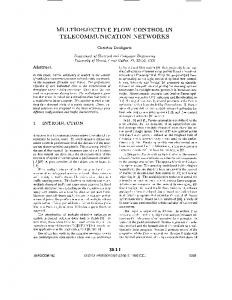
Figure 1.1: Illustration of payment architecture. Note that the authentication server is only involved at the beginning and end slots of a session. Steps: (a) The client reveals root of pay chain, x0 ; the authentication server verifies that validity of x0 . (b) The client reveals x1 , x2 , ... as time slots pass. (c) The access point deposits his payments by passing xT to authentication server. time slot were only on the order of a few minutes or less, it is likely that the transaction overhead would be comparable in size to the size of the payment itself. Clearly, such a high payment overhead would be prohibitive. Much work has been done in the area of making small payments, or micropayments, with a minimum of overhead. One scheme in particular appears to be promising in this context. The PayWord scheme, proposed by Rivest and Shamir, [1, 2] makes it possible for the payee, in our case the access point, to aggregate many payments from a client into a single, larger payment. The scheme works on the principle of pay chains. In the brief description that follows, we assume the reader is familiar with the ideas of digital signatures and one way functions. For a review of these concepts, the reader can consult [3]. Figure 1.1 illustrates how the PayWord scheme can be used in WiFi access point charging. Prior to beginning a session, a client would compute what the authors

7 of [1] calls an “H-chain” by repeated evaluation of a one-way function H. (A one-way function is a function that is relatively easy to compute, but whose inverse is extremely difficult to compute.) Specifically, the “H-chain” consists of values x0 , x1 , ..., xT where xt−1 = H(xt ) for t = 1, 2, ..., T . A client begins a session by passing the access point the root of the chain x0 that has been signed with the client’s digital signature. In each subsequent time slot, the client makes another payment by passing the next consecutive value of the H-chain to the access point. When the access point is ready to deposit the micropayments, the access point can combine them into single deposit by passing to the bank the client’s digitally signed x0 and the value, xT . The bank can verify the authenticity of x0 by its digital signature, and can verify that T micropayments were made by verifying that H T (xT ) = x0 . The most important property of this payment scheme, is that it does not involve a third party for each micropayment. The access point need only contact a certificate authority at the beginning of the session to verify the authenticity of the client’s digital signature of x0 . The access point can independently verify the authenticity of successive micropayments by verifying xt = H(xt+1 ).

1.5

Security Issues

Security is another critical issue that the P2P model of WiFi access faces. A client needs to know that the access point owner is not eavesdropping on her traffic, or spoofing the websites that she is trying to reach. Similarly, an access point needs to know that a client cannot use her access to launch an attack on his network. We believe that most

8 of these concerns can be addressed by existing techniques. For example, the client could use a secure tunnel to a home agent on the client’s home network to prevent the access point from eavesdropping or spoofing. The access point could use a firewall to prevent the client’s traffic from going beyond the access point and gateway router into the rest of the access point owner’s network. A harder problem is preventing the client from overusing the access point owner’s link to the Internet. Though the access point might rate limit the client’s incoming traffic to prevent the Internet uplink from being overused, the client might overuse the downlink, or even deliberately overuse the downlink in a form of denial of service attack against the access point owner’s network. One solution might be to measure the client’s downlink usage, and terminate her service if her usage is excessive. For the rest of this paper we will assume that these security issues are solvable and instead focus on the strategic interactions between an access point that is free to set and change prices over time, and a client seeking to maximize her utility.

1.6

Previous Work

Our model is that of an single access point, or seller, and a single buyer, the client. In the economics literature, a model with a single buyer and seller is called a “bilateral monopoly.” The static case of bilateral monopoly, the case where repeated transactions over time are not explicitly modelled, is well known and is found in economics text books [4]. What differentiates our model from the standard, static bilateral monopoly model is that we model our situation as a multi period dynamic game, where players have to consider the effects of their actions on the future as well as the present. There has been

9 some other work in studying bilateral monopoly situations using dynamic games. For example, Vincent looks at a bilateral monopoly in which buyers may either be low or high valuation types, while the seller tries to learn the buyer’s type from his behavior over the duration of the game [5]. The literature in bargaining, where two parties negotiate for a share of a surplus over multiple periods, is also closely related to dynamic, bilateral monopoly models [6, 7]. However, as far as we are aware, there is no prior work in either dynamic game models of bilateral monopoly or bargaining that capture the key features of the models we develop in this work. The networking community has also focused a lot of attention on pricing ideas in recent years. For example, many researchers have looked at congestion pricing, where resources, often network links, are priced according to how heavily they are being used, so that users are incentivized to redirect traffic to less congested, less costly links, or to lower the bit rates of their flows [8, 9]. At this point, our models do not look at how prices can be used to reduce congestion, but instead look at the strategic relationship between a buyer and seller. Network researchers have also looked at using mechanism design principles to incentivize users to bid their true utilities for network services [10, 11, 12]. The mechanism design methodology assumes a “principal” player who collets the player’s bids and is trustworthy. In contrast, our game model assumes that the access point and client face each other in the game without oversight of a neutral principal. Other networking researchers have applied game theory to congestion pricing [13], and splitting revenue between multiple providers [14], but none of these models capture all of the aspects of the structure of the Wi-Fi pricing situation we study in this work.

10

1.7

Overview

In Section 2.1 of the subsequent chapter, we introduce our basic two-player game model. In Section 2.2 we discuss an instance of the basic model that we call the web browsing model, and show that the provider or access point should charge his client a constant price. We also show how the web browsing model can be extended to a multi-hop scenario. In Section 2.3 we introduce the file transferor model, and show that if the access point has an a priori bound on the possible length of the client’s file, the client’s dominant strategy is to refuse any price greater than zero until the final time slot of her file transfer. The access point, in turn, charges a price of zero, until a critical slot t∗ is reached, and then tries to charge for the whole session in one shot. In Section 2.4, we study a model in which the access point is unsure whether he faces a file transferor or web browser client. In Section 2.4.1, we investigate what happens when a file transferor type client’s file length has no a priori bound. Chapter 2.5 summarizes and assesses the results of our basic model in all of its forms. Finally, Chapter 3 introduces some early-stage work in which we extend the basic model to address clients that can make repeat visits.

11

Chapter 2

Game-Theoretic Analysis 2.1

Basic Model

We can formulate the interaction between a access point and paying client using a simple two-player game model. The game progresses in discrete time slots or “periods.” At the beginning of the first time slot, the access point proposes an access price, p1 for access during the first time slot. The client can either accept the price and connect, or reject the price and not connect. If the price is rejected, the game ends and both client and access point receive zero payoff. In general, the access point offers connectivity at the beginning of time slot t at price pt . The game ends the first time the client rejects the access point’s proposal. The client’s utility function F (T, τ ) is a function of the number T of time slots the client chooses to connect and a parameter τ which we call the client’s intended session length. T is a decision variable; it is a function of the actions the client takes in each time slot, specifically the number of slots the client chooses to connect. In contrast τ is a type

12 variable that specifies the maximum time the client would be interested in connecting. For instance if the client were sitting on a park bench with a laptop and needed to leave the bench in 30 minutes, and the slot time were 1 minute, then τ would have a value of 30. The client does not choose τ in the game, but instead it is determined for the client by outside circumstances. The client knows the value of τ at the beginning of the game while the access point only knows its probability distribution. The client’s net payoff is F (T, τ )− PT

t=1 pt .

PT

t=1 pt ,

while the access point’s net payoff is

The underlying assumption is that the access point’s marginal cost to provide

the service to the client is negligible. We study the Nash equilibria of this game, under different assumptions of the structure of the utility function F (T, τ ). We assume the reader has some knowledge of game theory in the discussion that follows. A reference for the subject is [15]. In particular, we make use of the concept of perfect Bayesian equilibrium (PBE). A PBE, like a subgame perfect Nash equilibrium, is a strategy profile – or specification of each player’s strategy – such that no player can increase her expected payoff by unilaterally deviating from her PBE strategy at any point in the game. The important feature that distinguishes a PBE from a subgame perfect equilibrium is that, in this context, the access point maintains and refines conditional probability distributions on the random type-variables that describe the client. In general, a strategy specification of a dynamic Bayesian game is a mapping from a player’s type, and a player’s information set to an action, or in a mixed strategy, to a distribution among possible actions [15]. Assuming players have “perfect recall,”

13 the information set is the history of actions the player has observed. In our model, if the game reaches slot t, then the history is completely specified by the previous prices charged. Thus, a pure strategy for an access point is simply a price sequence. An access point’s mixed strategy, or behavior strategy, is a probability distribution on prices to charge in each slot t dependent upon the prices actually charged in earlier slots 1,..., t − 1. For the client, a strategy is specified as a mapping from its type and information set to an acceptance decision, or to a probability of accepting.

2.2

Web Browsing Model

In this chapter we model a client browsing the web. The client’s utility is proportional to the length of time T that she gets to browse the web, but her utility saturates after the maximum intended session length τ is reached: F (T, τ ) = U · min(T, τ ).

(2.1)

The client’s type is specified by her utility per slot U and intended session length τ . The client knows the values for U and τ while the access point just knows their distributions. Theorem 2.1. Consider a web browser client with utility defined by definition (2.1). Suppose that U and τ are independent and finite-mean, and U has a continuous distribution. Then the following strategy profile is a PBE equilibrium. • The client connects or remains connected in slot t iff t ≤ τ and pt ≤ U . (We refer to this as the “myopic strategy.”)

14 • The access point charges a non-decreasing sequence of prices {pt } such that pt ∈ arg max pP (U ≥ p). p

Note that Theorem 2.1 says that an access point should pick its prices by looking at just the prior distribution of U . In fact, an important corollary to Theorem 2.1 is that it is a PBE for the access point to pick a single maximizing value of pP(U ≥ p), say p∗ , and charge the fixed price pt = p∗ in all time slots. This is somewhat surprising, because whenever a myopic client accepts price pt , the access point can refine its conditional distribution of U by lower bounding it by pt . One might have expected that an access point might want to try charging a higher price than pt after learning that the client’s utility is at least pt . Theorem 2.1 states this intuition is not correct. We now prove Theorem 2.1. Proof of Theorem 2.1. First, we find the access point’s optimal counter strategy to a client playing the “myopic strategy.” A pure strategy for the access point can be {1,2,...}

specified by a sequence of nonnegative prices {pt }∞ t=1 ∈ R+

to charge at each time

slot t ∈ {1, 2, ...}. The access point wishes to choose his sequence of prices to maximize his expected revenue, as expressed by: J1a ({pt }) =

∞ X t=1

pt P(U >

max pu )P(τ ≥ t).

u∈{1,...,t}

(2.2)

In the notation J1a ({pt }), the a superscript signifies that it is the expected revenue (objective) of the access point, the 1 subscript indicates that it is the objective from slot 1 onward, and the ({pt }) signifies that the objective is a function of the access

15 point’s price sequence. Expression (2.2) reflects that a client will be connected in slot t if and only if her utility per slot U is greater than the current price pt as well as all previous prices, p1 , ..pt−1 , and if the client’s intended session length τ is not less than t. We see that we can find a maximizing sequence of expression (2.2) even if we restrict ourselves to non-decreasing sequences. This is because for any sequence {˜ pt } for which there exists a u such that p˜u < p˜u−1 , we can define a new non-decreasing sequence {pt } with pt = max(˜ pt , ..., p˜1 ) and we would have J1a ({pt }) ≥ J1a ({˜ pt }). The same idea expressed in terms of the situation – an access point that has seen a myopic client accept a price pt knows that he can charge at least pt in slot t+1 without risking that he charges more than the client is willing to pay. For convenience, we define S + to be the set of nondecreasing price sequences, that is {pt } ∈ S + if {pt } ∈ R∞ + and pt+1 ≥ pt ∀t ∈ {1, 2, ...}. The access point wishes to choose a positive sequence of prices to maximize his expected revenue, as shown in the following expression: "

max J1a ({pt }) {pt }∈S +

= max

{pt }∈S +

∞ X t=1

#

pt P(U > pt )P(τ ≥ t) .

(2.3)

Because U and τ are finite mean, one can substitute their Markov bounds into expression (2.3) to show that the access point’s expected payoff against a myopic client is bounded [17]. Each term in the summation of expression (2.3) is a function of a different price, pt , so the entire sum can be maximized by independently maximizing each term in the summation. We note that arg maxp pP(U ≥ p) is non-empty because y(p) = pP (U ≥ p) is a continuous, nonnegative function, with y(0) = 0, and limp→∞ y(p) = 0, and thus must achieve a maximum on [0, ∞). So if the access point chooses each pt such that pt ∈ arg maxp pP(U ≥ p), with {pt } ∈ S + , then the access

16 point maximizes his expected payoff (2.3). Now looking at the client’s side, it is easy to see that the myopic strategy is a best response to an access point that never lowers prices. Because these strategies are best responses to each other, they constitute a (Bayesian) Nash equilibrium strategy profile. Now we will verify that the strategy profile is a PBE – that the strategy profiles remain best responses to each other in any continuation game, beginning at an arbitrary slot s. A client facing nondecreasing prices in this game will of course face nondecreasing prices in any continuation game starting at slot s, thus a client that expects nondecreasing prices should stick to the myopic strategy in the continuation game beginning at slot s. An access point that expects his client to be myopic should choose his prices in the continuation game to maximize Jsa ({pt }∞ t=s )

=

∞ X

"

pt P

U>

t=s

u u∈{s,...,t}

!

#

max p U > ps−1 × P(τ ≥ t|τ ≥ s) .

(2.4)

For any price sequence {˜ pt }∞ t=s which has prices that are less than ps−1 , we see that a p }∞ ). Thus the access point can maximize its reward Jsa ({max(˜ pt , ps−1 )}∞ t t=s t=s ) ≥ Js ({˜

to go by selecting its continuation game prices to be no smaller than ps−1 . Thus assuming pu ≥ ps−1 for all u ≥ s we may write, –

Jsa ({pt }∞ t=s )

∞ X 1 pt P P(U > ps−1 ) t=s

‚

U>

Œ

max pu

u∈{s,...,t}

™

1 × P(τ ≥ t) . P(τ ≥ s)

(2.5)

Note that expression (2.5) has a structure that parallels expression (2.2), with the exception of the scaling factors 1/P(U > ps−1 ) and 1/P(τ ≥ s) which have no dependence on the prices chosen from slot s forward. Thus the same argument that was used to show that expression (2.2) is maximized with a nondecreasing sequence with elements in

17 arg maxp pP (U ≥ p) can be used to show that expression (2.5) is also maximized with a nondecreasing sequence with elements in arg maxp pP (U ≥ p). Therefore we have shown that the access point strategy described in the statement of Theorem 2.1 is remains a best response to a myopic client in any continuation game. Our web browser result is similar to results shown in other contexts in the economics literature. For example, in [16] the authors show that under certain assumptions that it is not more profitable for a seller to condition pricing on the past behavior of the customer.

2.2.1

Web Browsing Examples

We now consider a few specific examples of the web browsing model. In the first example, suppose that the client’s per slot valuation, U , is distributed uniformly on [0, 1]. Then the unique maximizer of pP(U > p) would be 0.5, and thus the PBE specified by Theorem 2.1 is that the access point charges 0.5 in all slots, and that the client plays a myopic strategy. In the second example, suppose that the game started with U distributed uniformly on [0.5, 1]. The unique maximizer of pP(U > p) would be 0.5, and the access point should charge 0.5 in all time slots in PBE. We see that in this second example, the distribution of U , is the same as the conditional distribution of U in the first example, after a client accepts the price of 0.5 in slot 1. Thus the second example is equivalent to a continuation game of the first example, so it should be expected that the equilibrium prices should be the same. Finally, if U is distributed uniformly on [a, b], we find that the access point should charge max(b/2, a) in each slot, according to the PBE described by Theorem 2.1.

18

2.2.2

Uniqueness of the PBE

Theorem 2.1 shows that a strategy profile with the client playing a myopic strategy is a PBE, however it does not show that this strategy profile is the unique PBE. In the special case that the intended session length τ is bounded, we can show that the myopic strategy is the unique client strategy in PBE. Proposition 2.2. Suppose τ is distributed on {1, ..., n}, and U is finite mean, then the following characterizes all PBE: • The client follows a myopic strategy. • The access point charges a non-decreasing sequence of prices {pt } such that pt ∈ arg max pP (U ≥ p). p

Proof. In slot n, the client’s dominant strategy is the myopic strategy. This is simply because there is no future after slot n, so the client should myopically maximize her expected return in slot n After deleting the client’s dominated strategies, the access point’s dominant counter strategy in slot n is to charge at least max(p∗ , p1 , ...pn−1 ). Where p∗ = min(arg max pP (U ≥ p)) p

. In slot n − 1, the client can anticipate the access point’s action in slot n. The client knows that pn ≥ pn−1 . Facing non-decreasing prices on {n − 1, n}, the client’s dominant strategy in slot n − 1 is the myopic strategy.

19

Internet

Client

Reselller

Access Point

t

Figure 2.1: Multi-hop scenario: Client, Reseller, and Root Access Point.

Suppose we have shown that for each slot u ≥ t, the access point charges at least max(p∗ , p1 , ...pu−1 ), and the client plays the myopic strategy in slot u. In slot t − 1, the client knows that prices {pt−1 , ..., pn } will be a non decreasing sequence. The client’s dominant strategy in slot t − 1 is therefore the myopic strategy. The access point thus charges at least max(p∗ , p1 , ...pt−2 ). By induction, the client plays the myopic strategy in all time slots. The access point’s best response is to charge a non-decreasing sequence of prices {pt } such that pt ∈ arg maxp pP (U ≥ p).

2.2.3

Multiple Hops

Having considered a single-hop model in which an access point sells access directly to a client, we now consider a scenario where a “root” access point sells service to a reseller, which in turn sells the service to an end client with a web browser utility. This situation arises when a client is not within communicating range of an access point with a wired Internet connection, and instead needs an intermediate node, or reseller in our

20 terminology, to act as a relay. The situation is depicted in Figure 2.1. As shown in Figure 2.1, the client tries to begin a session by sending a request for service to the reseller. In order to serve the client’s request, the intermediate node sends its own request for service to the “root” access point that has a wired Internet connection. The root access point passes the reseller a price for the first slot, c1 , which the reseller can either accept or reject, and as in the single-hop game, the game ends upon the first rejection. Before deciding to accept or reject the c1 price, the reseller sends its first slot-price, called p1 , to the client. If the client accepts p1 , the reseller would accept the c1 price from the root access point. If the client rejects p1 , and assuming that the reseller had no other use for connectivity with the access point than to serve the client, the reseller would reject the c1 price and the game would end. If the client and reseller accept their offers in slot t, the game continues into slot t + 1 with the root access point choosing a price ct+1 to offer the reseller, and the reseller choosing a price pt+1 to offer the client. As in the single-hop model, in this game there is also a notion of intended session length, which is the length of time after which the client stops earning utility from remaining connected. The intended session length is a random variable τ with its sample value known to the client, and only its distribution known to the other parties. Thus the client’s utility is described by expression (2.1), where T is the number of slots the client chooses to remain connected. The clients payoff is simply her utility minus what she pays, F (T, τ ) −

PT

t=1 pt .

The re-seller’s payoff is simply the difference of the

payments he receives and the payments he makes,

PT

t=1 (pt

− ct ), while the access point’s

21 payoff is the sum of all payments he receives from the reseller,

PT

t=1 ct .

As in the single-hop game, a client’s pure strategy is specified as a mapping from her type and information set to an acceptance decision. A pure strategy for the access point is specified as a sequence of prices c1 , c2 , ... to charge in each time slot. In general, a pure strategy for the reseller is a mapping from prices he has been charged c1 , ..., ct , as well as the prices the reseller charged in the past, p1 , ..., pt−1 , to a price to charge in the current slot, pt . For convenience, we denote the reseller’s history as △ €

Š

hrt = {cu }tu=1 , {pu }t−1 u=1 . Thus a pure strategy for the reseller is a specification of the functions pt (hrt ). Having identified what the strategy spaces for the three players look like in general, we now identify a specific strategy profile that is a PBE. Theorem 2.3. The following strategy profile is a PBE: • The client follows a myopic strategy, connecting iff t ≤ τ and pt ≤ U . • The reseller picks a function p∗ (c) that satisfies the properties: p∗ (c) ∈ arg max(p − c)P(U > p)

(2.6)

p∗ (c′ ) ≥ p∗ (c)

(2.7)

p

∀c′ > c

and charges the price pt (hrt ) = p∗ (ct ) in slot t. • The access point charges a non decreasing price sequence {ct } with ct ∈ arg max [c · P(U > p∗ (c))]. c

22 Note that in the equilibrium reseller strategy profile detailed in Theorem 2.3, the choice of price is just a function of his current cost ct . This is significant because in general the reseller’s price strategy can in general depend on the past costs c1 , ..., ct−1 as well. We now state and prove a Lemma that we will later use in the proof of Theorem 2.3. Lemma 2.4. There exists a function p∗ (c) that satisfies properties (2.6) and (2.7). Proof of Lemma 2.4. Define △

yc (p) = (p − c)P(U > p). yc (p) is a continuous function with yc (c) = 0, yc (p) ≥ 0 for p > c, and has limp→∞ yc (p) = 0. Thus, yc (p) must achieve a maximum value somewhere on [c, ∞). Thus arg maxp yc (p) is a non empty set. We find p∗ (c) by construction. Set 

∗

‹

p (c) = min arg max yc (p) . p

Note that p∗ (c) is well defined for all c > 0 because arg maxp yc (p) is non empty. It remains for us to show that p∗ is monotonic non-decreasing, which we will do by contradiction. Suppose it were not monotone non-decreasing. Then their exists (cl , ch ) : cl < ch with p∗ (ch ) < p∗ (cl ). For convenience, we define pl = p∗ (ch ) and ph = p∗ (cl ) so that pl < ph . It must be that (ph − cl )P(U > ph ) > (pl − cl )P(U > pl )

(2.8)

or else ph would not be the lowest valued maximizer of ycl (·). It also must be that (pl − ch )P(U > pl ) ≥ (ph − ch )P(U > ph )

(2.9)

23 or else pl would not be the lowest valued maximizer of ych (·). Combining (2.8) and (2.9) we have pl − ch p l − cl > . ph − ch p h − cl

(2.10)

But expression (2.10) implies pl cl + ch ph < ch pl + ph cl . Regrouping terms we get ph (ch − cl ) < pl (ch − cl ), which is a contradiction. Thus the p∗ (c) we constructed must be monotone non-decreasing, and thus we have found a function that satisfies (2.6) and (2.7). With Lemma 2.4 proved, we may now prove Theorem 2.3. Proof of Theorem 2.3. We begin the proof of Theorem 2.3 by showing that if an access point charges the reseller a sequence of prices {ct } ∈ S + where S + is the set of nondecreasing sequences, and if the client plays the myopic strategy, then it is a best response for the reseller to use the strategy pt = p∗ (ct ) where the function p∗ (c) has the properties (2.6) and (2.7). The reseller should choose a mapping from history hrt to price pt to maximize expected reward: J1r

({pt (hrt )}; {ct })

=

∞– X t=1

‚

(pt − ct )P

U>

Œ

max pu

u∈{1,...,t}

™

× P(τ ≥ t) .

(2.11)

24 The “; {ct }′′ notation in J1r ({pt (hrt )}; {ct }) signifies that the reseller objective function is dependent upon the reseller’s assumption of the access point’s strategy, which for pure strategies can be specified as the sequence {ct }. Define a modified objective △ J˜1r ({pt }; {ct }) =

∞ X t=1

(pt − ct )P(U > pt )P(τ ≥ t).

(2.12)

Note that J1r |{pt }∈S + ({pt }; {ct }) = J˜1r |{pt }∈S + ({pt }; {ct })

(2.13)

J1r ({pt }; {ct }) ≤ J˜1r ({pt }; {ct }).

(2.14)

and

Now suppose the reseller picks a function p∗ (c) satisfying properties (2.6) and (2.7) and uses the strategy pt (hrt ) = p∗ (ct ). Then for every {ct } ∈ S + , pt (hrt ) = p∗ (ct ) maximizes expression (2.12) because the sum is separable and can be maximized term by term. Furthermore, expressions (2.13) and (2.14) imply that pt (hrt ) = p∗ (ct ) also maximizes expression (2.11) for all possible {ct } ∈ S + . Thus the strategy pt (hrt ) = p∗ (ct ) is a best response to a myopic client and access point that does not decrease prices. Next we show that this strategy remains the best response in all continuation games. Suppose the reseller reaches slot s having used the strategy pt (hrt ) = p∗ (ct ), the reseller wishes to maximize the expected reward to go:

Jsr ({pt (hrt )}; {ct }) = ∞ X t=s

"

(pt − ct ) P

U>

u u∈{s,...,t}

!

#

max p U > ps−1 × P(τ ≥ t|τ ≥ s) . (2.15)

25 From expression (2.15), we see that an access point can maximize his expected reward to go by considering only prices greater than or equal to ps−1 , thus we may write: Jsr ({pt (hrt )}; {ct }) =

–

∞ X 1 (pt − ct ) P P(U > ps−1 ) t=s

‚

Œ

U>

max pu

u∈{s,...,t}

™

1 × P(τ ≥ t) . (2.16) P(τ ≥ s)

The objective in expression (2.16) differs from expression (2.11) only by factors [P(U > ps−1 )]−1

and

[P(τ ≥ s)]−1

which have no dependence on the prices chosen from slot s forward. Thus, the same arguments used to show that the strategy pt (hrt ) = p∗ (ct ) is a best response starting from time slot 1 can be used to show that it is also a best response starting from time slot s. Next we look at the access point strategy. We assume the client is myopic, and that the reseller uses the strategy pt (hrt ) = p∗ (ct ). The access point wishes to maximize his expected revenue J1a ({ct }; {pt (hrt )})

∞ X

ct P(U >

=

t=1

max p∗ (cu ))P(τ ≥ t).

u∈{1,...,t}

Because p∗ (c) is monotone, we can invert it and define the random variable V = p∗−1 (U ). Now, the access point’s objective becomes J1a ({ct }; {pt (hrt )})

=

∞ X

ct P(V >

t=1

max cu )P(τ ≥ t).

u∈{1,...,t}

(2.17)

Expression (2.17) is identical in structure to expression (2.2), which describes the expected payoff of an access point in the single hop model. Thus from the access point’s perspective, the multi-hop scenario in which the access point sells to a reseller which in

26 turn sells to a client with a utility per slot U is equivalent to selling directly to a client with its utility per slot distributed like V . Thus the same argument used in the proof of Theorem 2.1 to verify the best response of the access point in the single-hop scenario can be re-used here to show that a best response of the access point would be to pick a sequence of prices {ct } with ct ∈ arg maxc P(V > c). Finally we observe that if the root access point charges a nondecreasing price, and that the reseller’s price is a static function of access point price, then the client’s best response is to play a myopic strategy. This is because the client’s best response to non-decreasing prices is a myopic strategy.

Example of Multi-hop Equilibrium The sharing of revenue between the reseller and access point is similar to that of the leader and follower in the classic Stackelberg competition game. In the Stackelberg game, a leader and follower firms successively decide how much of a good to produce, and then the market price of the good is determined by the sum of the two firms productions and a demand function [18]. In the model developed here the access point, analogous to the “leader,” chooses a price ct , while the “follower,” or reseller, chooses a markup over the access point’s price, pt − ct . The client’s probability of accepting is a function of the sum of the leader’s and follower’s choices. In the Stackelberg game, the leader makes at least as much revenue as the follower in equilibrium. By analogy, we can observe that the access point’s share of the revenue should be greater than or equal to the reseller’s revenue in equilibrium. For instance, supposing that the client’s distribution of U were uniform on [0, 1], in the PBE

27 characterized by Theorem 2.3, the access point would charge 0.50 in each time slot, while the client would charge 0.75. In this example the access point would have an expected revenue twice that of the access point.

2.3

File Transfer Model

Here we model a situation in which a client is downloading a file, and the client must remain connected for the entire duration of the file, or in our terminology the intended session length, to earn any utility for the file. The client’s utility function has the form: 8 > >
> :

0

if T < τ

Uτ

if T = τ

(2.18)

The client’s type is determined by the two random variables τ and U , where τ is the intended session length, in this case the length of the file, and U is the client’s utility per unit of file length. Theorem 2.5. Suppose the client has a file transfer utility function as in expression (2.18), with U a continuous random variable on [l, h] with 0 ≤ l < h, and the session length τ , distributed on {1, ..., n}. Both U and τ have sample values known to the client, and unknown to the access point. We also assume that U and τ are finite mean, and that U is continuously distributed. Then the following characterizes all perfect Bayesian equilibria:

• The client plays a “pessimistic” strategy: The client accepts in slot t < τ iff pt = 0. When t = τ , the client connects if she had been connected in all of the previous slots, and pt < U τ . (She never connects if pt > U τ but may connect if pt = U τ .)

28 • The access point charges

8

pt =

> >
> :

u ∗ t∗

otherwise

(2.19)

where(u∗ , t∗ ) ∈ arg max utP (U > u, τ = t). (u,t)

Proof. The proof uses backwards induction, and iterated deletion of dominated strategies. We begin by showing that clients with intended session length n follow the pessimistic strategy. Suppose the client has an intended session length of n and utility parameter U = u. We will refer to such a client as a type (u, n) client. When the game reaches slot n, a type n client’s dominant strategy is to accept any price less than nu, because doing so would earn her a payoff greater than if she refused to finish her transfer in the last slot. Because U is lower-bounded by l, the access point should charge at least nl in slot n. More specifically, after deleting his client’s dominated strategies, and deleting the access point’s own dominated strategies, the access point’s remaining strategies involve charging at least nl. Knowing that a access point will charge at least nl in the last slot, clients of types ([l, l + nǫ ), n) will be unwilling to pay more than ǫ in any slot before their last slot, n. Otherwise, such clients would predictably end up paying at least ln + ǫ and would finish the game with negative payoff. We refer to this as an ǫ-pessimistic strategy. Now suppose a client of unknown type were to stay connected up until slot n, and in at least one slot prior to n did pay ǫ or more. The access point would deduce that the client can not be of types ([l, l + nǫ ), n), because such clients play an ǫ-pessimistic

29 strategy. Therefore, the access point deduces that the client’s type must be in the range([l + nǫ , h], n) and charges at least ln + ǫ, knowing that all clients in the type range would be compelled to pay. Knowing that a access point would charge at least nl + ǫ in the last slot, clients of type ([l, l +

2ǫ n ), n)

also play an ǫ-pessimistic strategy.

Supposing that we have shown by iterated deletion of dominated strategies that an access point would charge at least nl + tǫ in the last slot. Consequently, clients of types ([l, l +

(t+1)ǫ n ), n)

play an ǫ-pessimistic strategy. A access point in slot n facing a

client of unknown type can eliminate the possibility that his client’s type is in the range ([l, l +

(t+1)ǫ n ), n),

and thus charge at least nl + (t + 1)ǫ.

By induction clients of types ([l, h], n), play an ǫ-pessimistic strategy, and this is true for any ǫ > 0. The only strategy for which this is true for all ǫ > 0 is the “pure” pessimistic strategy of accepting a maximum price of 0 in slots prior to the final slot of the file transfer. We now prove the induction step. Suppose we have shown that Clients of Types ([l, h], j) through types ([l, h], n) follow the pessimistic strategy. We show it for Type ([l, h], j − 1):

Suppose that a type ([l, h], j − 1) client does not play the pessimistic strategy by accepting a nonzero price in a slot with index less than j − 1. When the game reaches slot j − 1, the access point can deduce that the client is of type j − 1 or greater, and that clients of type j or greater would have already quit the game. Thus, the access point knows he faces a type j − 1 client. Knowing his client’s file ends in slot j − 1, the access

30 point can charge (j − 1)l and be assured that the client will be compelled to pay. Thus clients of types ([l, l + nǫ ), j − 1) will be unwilling to pay more than ǫ in any slot before their last slot, j − 1. Continuing this argument inductively in exactly the same way as we did to show that clients of type ([l, h], n), are ǫ pessimistic we can show that clients of type ([l, h], j − 1) are ǫ pessimistic. The only strategy that is ǫ pessimistic for all ǫ > 0 is the ‘pure” pessimistic strategy of accepting a maximum price of 0 in slots prior to the final slot of the file transfer. Thus, clients of type ([l, h], j − 1) are pessimistic. By induction, clients of all types play the pessimistic strategy. Access Point counter strategy: An access point facing pessimistic clients has only one chance to charge nonzero prices. The access point charges according to expression (2.19) where (u∗ , t∗ ) ∈ arg max utP (U > u, τ = t). (u,t)

Note that one can show that arg max(u,t) utP (U > u, τ = t) is nonempty by using the fact that U and τ are finite mean.

2.3.1

Inefficiency of the File Transfer Model Equilibrium

The equilibrium described by Theorem 2.5 is very inefficient. If the client’s intended session length is greater than t∗ , in equilibrium the access point would be forced to charge 0 in the slots prior to t∗ , and then at time t∗ , the client will refuse to pay the access point’s price. If the client’s intended session length is less than t∗ , in equilibrium the client will finish her file download without paying anything. Only when the client’s intended session length is exactly t∗ will the access point earn any revenue.

31

2.4

Bayesian Model

In Chapter 2.2, we found that when a client has a web browsing utility as described by expression (2.1) that an access point charges a constant price in PBE. In Chapter 2.3, we discovered that when a client has a file transferor utility as described by expression (2.18), that an access point does not charge a constant price in PBE. In this chapter, we study the case in which the access point does not know if his client is a file transferor or a web browser. We model this situation by assuming that the access point begins the game knowing the prior probability x that the client is a file transferor. We call this combined model simply the Bayesian Model. Although, we would like to find a general solution to the Bayesian Model without making any assumptions about the probability distributions of the intended session length τ , and the utility per slot U , we are most interested in knowing whether the price is constant in PBE. When x is 0, the Bayesian Model is equivalent to a “pure” web browsing model, so constant price is a PBE by Theorem 2.1. When x is 1, the Bayesian Model is equivalent to a “pure” file transfer model, where we know that constant price is not a PBE. Based on these facts, one might hypothesize that when x has a small enough value, constant price is a PBE. We will show by studying an example, in which we choose specific distributions for τ and U , that this hypothesis is not correct. We state the example, and the results of its analysis in Proposition 2.6 which follows. Proposition 2.6. Suppose that the client is a file transferor (FT) with probability x and a web browser (WB) with probability 1 − x. The access point knows the value of x, while the client knows her true type. Also suppose that clients of both types have an

32

Equilibrium Strategy Profile s* Equilibrium Strategy Profile sp

1

0.8 pp 2

p*

2

Price

0.6

p*

1

0.4

0.2

pp 1

0

0

0.1

0.2

0.3 0.4 0.5 0.6 0.7 x: Probability Client is a File Transferor

0.8

0.9

1

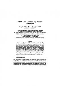
Figure 2.2: PBE prices for the 2 time slot Bayesian game described in the statement of Proposition 2.6.

intended session length of τ = 2, and this is known to both parties. The utility per slot U is uniformly distributed on [0, 1]. The client knows the sample value of U while the access point (AP) knows only the distribution. The utility functions for WB and FT type clients are given by expressions (2.1) and (2.18) respectively. Then the following three assertions are true: 1. The strategy profile (pair of player strategies), s∗ = (s∗AP , s∗C ) is a PBE ∀x ∈ [0, 0.516], where the access point strategy, s∗AP , and the type dependent client strategy, s∗C , are defined as follows: • s∗AP : Charge the price sequence {p∗1 , p∗2 } in the 2 slots of the game, where the prices p∗1 and p∗2 are dependent on x as : p∗1 =

4−5x 2(1−x)(4−x) ,

p∗2 =

4−3x 2(1−x)(4−x) .

• s∗C (WB): (WB clients) Connect in slot 1 iff p1 ≤ U . Connect in slot 2 iff connected in slot 1 and p2 ≤ U . Note that this is a myopic strategy.

33 • s∗C (FT): (FT clients) Connect in slot 1 iff p1 + pˆ2 ≤ 2U where pˆ2 , intuitively the price the client expects in slot 2, is equal to p∗2 . Connect in slot 2 iff connected in slot 1 and p2 ≤ 2U . √

2. The strategy profile, sp = (spAP , spC ) is a PBE ∀x ∈ [ 3−2

5

≈ 0.382, 1], where the

player strategies are defined as: 1 }. • spAP : Charge the price sequence {0, 2−x

• spC (WB): The myopic strategy, ∗ sP C (WB) = sC (WB).

• spC (FT): The pessimistic strategy – connect in slot 1 iff p1 = 0 and connect in slot 2 iff connected in slot 1 and 2U ≥ p2 . (Note that we chose the superscript p in sp to signify that FT clients are pessimistic in this strategy profile.) 3. For x > 0 there are no PBE in which the AP charges a constant price (p1 = p2 ). The prices of the two equilibrium strategy profiles described by Proposition 2.6 are shown in Figure 2.2. Proof. We begin by showing that s∗ is a PBE. First we consider whether the client’s strategy s∗C is a best response to the access point strategy s∗AP . The access point prices are nondecreasing in s∗AP , and we have seen that a web browser’s best response to nondecreasing prices is a myopic strategy, so s∗C (WB ) is a best response. Similarly, when the AP plays s∗AP , playing s∗C (FT ) gives the highest possible payoff to a FT client for all

34 possible values of U . Furthermore, a FT client does not benefit by unilaterally deviating in the continuation game beginning in slot 2. Next we consider whether s∗AP is a best response to s∗C . We begin by writing an expression for the access point revenue R(p1 , p2 ) assuming that clients play s∗C : h



R(p1 , p2 ) = p1 (1 − x)G(p1 ) + xG h

p1 +p∗2 2



h

p2 (1 − x)G (max[p2 , p1 ]) + xG max

i

+ p1 +p∗2 p2 2 , 2

ii

where G(p) = P(U > p) = max((1 − p), 0). R(p1 , p2 ) is piecewise quadratic in (p1 , p2 ). By breaking up R(p1 , p2 ) into quadratic functions on different regions of R2 , finding the maxima on each region, and then finding the global maximum across all of the regional maxima, it can be shown that (p∗1 , p∗2 ) is the unique maximizing value of R(p1 , p2 ) for x ∈ [0, 0.516], where 0.516 is a decimal approximation to the root of a 6th order polynomial. Thus (p∗1 , p∗2 ) is the AP’s best response to clients that play s∗C , for x ∈ [0, 0.516]. (Note that for values of x larger than ≈ 0.516, s∗AP is not a best response because the AP can earn greater expected revenue by charging a different set of prices than (p∗1 , p∗2 ). ) To see that the access point has no incentive to deviate from s∗AP in the continuation game beginning at slot 2, we can use Bayes’ Rule to find that the AP’s expected revenue in slot 2, given the client accepted price p∗1 in slot 1. After a few transformations we have, J2a (p2 ) =

h

R(p∗1 , p2 )

p∗1 (1 − x)G(p∗1 ) + xG

 ∗ i p1 +p∗2

2

− p∗1

which is maximized when p2 = p∗2 . Next we show that sp is a PBE. Under the prices of spAP , clients following spC connect whenever connecting will result in a positive payoff, and do not connect

35 otherwise. Thus spC is a best response to spAP , and furthermore the client’s best response in the continuation game beginning in slot 2 is to not deviate from spC . With clients playing spC , an AP can charge 0 in the first slot, and keep the FT clients connected, or choose a nonzero price and earn revenue from only the WB clients. If the AP chooses the latter option, then he should maximize expected revenue from WB clients, which he can do by charging

1 2

in both slots, earning him an expected revenue

of (1 − x) 21 . If the AP chooses 0 for its slot 1 price, then both FT and WB clients would be potential customers in the 2nd slot, and the AP’s optimal 2nd slot price is found by maximizing €

p2 (1 − x)P(U ≥ p2 ) + p2 xP U ≥ which happens at p2 =

1 2−x ,

p2 2

Š

earning an expected revenue of

1 4−2x .

The latter option

1 }, which is the same as the spAP strategy defined in the statement of of charging {0, 2−x

Proposition 2.6, earns more expected revenue than the option of charging √

1 2

in each slot

√

for x ∈ [ 3−2 5 , 1]. Thus spAP is a best response to spC for x ∈ [ 3−2 5 , 1]. Though we have shown that the strategy profiles s∗ and sp are PBE for particular ranges of x, we have not yet shown that there is not another PBE where the access point charges a fixed price p1 = p2 . Let us suppose the AP does follow the strategy of charging p1 = p2 = p, and look for a contradiction. The best response for both FT and WB clients is to follow a strategy of accepting in slot 1 whenever U > p. When a client accepts in first slot, in the next slot the AP faces a client with U > p, and a posterior probability, x of being a FT type. In the continuation game beginning at slot 2, a FT client has a dominant strategy of accepting whenever 2U > p2 , while a WB client has a

36 dominant strategy of accepting whenever U > p2 . Thus an access point that wishes to charge constant price should choose that price to maximize €

Š

2p(1 − x)P(U ≥ p) + pxP (U ≥ p)[1 + P U ≥ p2 |U ≥ p ] which occurs at p′ = 12 . However in the continuation game beginning at slot 2, the access point maximizes revenue by maximizing €

p2 (1 − x)P(U ≥ p2 |U ≥ p) + p2 xP U ≥

p2 2 |U

≥p

Š

1 ). Thus for x > 0 and p′2 > p′ , the access point wants to which occurs at p′2 = max(p, 2−x

deviate from the constant price strategy and charge the higher price p′2 . Thus we have shown that constant price is not a PBE for x > 0. We make a few observations about whether the equilibria identified in Proposition 2.6 are unique. When x = 0, the model is equivalent to a pure web browsing model, and Proposition 2.2 applies, telling us that the PBE is unique, and price is constant. The equilibrium strategy profile s∗ covers this case because p∗1 = p∗2 =

1 2

when x = 0.

When x = 1, the model is equivalent to a pure file transferor model, and we can use Theorem 2.5 to say that the unique PBE is one in which FT clients are pessimistic. This PBE is the same as sp from Proposition 2.6. For 0 < x < 1 it is possible, and indeed likely, that there are other PBE that we have not identified here. However, as we stated and showed in Proposition 2.6, when x ∈ (0, 1] there is no PBE for which the access point charges constant price. Though price is not constant in PBE for x > 0, the PBE described by s∗ has the access point charging prices that are “reasonable” in that they there is a nonzero

37 probability that a client’s single slot utility exceeds each price. This is in contrast to the PBE of the pure file transfer model in which the access point tries to charge for the whole value of a file in a single slot. In the section that follows, we study whether prices are “reasonable” when file lengths have unbounded distributions.

2.4.1

Unbounded Length

In Chapter 2.3 we found that when file transferor clients have file lengths picked from a bounded distribution, clients are pessimistic and that the access point does not charge a constant price. In Chapter 2.4, we studied a Bayesian Model that combines the file transfer and web browsing models, and in an example where file length is bounded, we found that the access point price is not constant. In this section we study what happens in PBE when the file length is not picked from a bounded distribution. In Theorem 2.7 which follows, we find that for a Bayesian Model in which intended session length has an unbounded distribution, it is not a PBE for the access point to charge “reasonable” prices in every slot. Where we say a price is “reasonable” if it has a nonzero probability of being less than a client’s single slot utility. Note that Theorem 2.7 implies that it is not a PBE for an access point to charge constant price. In the statement of Theorem 2.7 we make modest assumptions about the distribution of τ which hold, for example, for the geometric distribution. Theorem 2.7. Suppose that: • The intended session length τ is distributed on{1, 2, ...}. • With probability x > 0 the client has a file transferor (FT) utility function F (T, τ ) =

38 U τ · 1(T ≥ τ ). • With probability 1 − x, the client has a web browser (WB) utility function F (T, τ ) = U min(T, τ ). • U is positive, continuously distributed, and independent of τ , and whether the client is of type FT or WB. • The distribution of τ is independent of whether the client is of type FT or WB, and there exists constants α > 0 and δ > 0 such that for all t > 0, P(τ = t|τ ≥ t) > δ E[τ − t|τ ≥ t] < α. Then in PBE the access point (AP) price in each time slot is not bounded by any constant h for which P(U > h) > 0. Proof. Suppose the strategy profile s = (sAP , sC ) is a PBE in which the access point prices are never more than h. For convenience, we define ǫ = P (U > h). If the game reaches slot t, the AP can consider deviating from sAP at slot t by charging a price of ht to exploit FT clients whose transfers are finishing in slot t. The one-step expected revenue for such a deviation is htP(Client = FT , τ = t, U > h|τ ≥ t, dt−1 = C)

(2.20)

where the notation {dt−1 = C} signifies the event in which the client is connected after slot t − 1. Using Bayes’ Rule, the independence of the type variables, and the fact that

39 FT clients will always be connected in slot t − 1 when U > h and τ ≥ t, we write the following inequalities to bound expression (2.20): P(Client = FT , τ = t, U > h|τ ≥ t, dt−1 = C) =

P(Client = FT , τ = t, U > h, dt−1 = C|τ ≥ t) P(dt−1 = C|τ ≥ t)

≥ P(U > h, Client = FT , τ = t|τ ≥ t) = xP(U > h)P(τ = t|τ ≥ t) = xǫδ.

(2.21)

Thus, using expression (2.21) we see that the deviation of charging ht at time t earns at least htxǫδ. Now we attempt to characterize the expected revenue an AP earns for sticking to strategy sAP at time t. Under sAP , the expected revenue to go from time t forward, which we call Jta (sAP ), cannot be more than if AP receives h in all the remaining time slots of the client’s session length. Thus Jta (sAP ) < hE[(τ − t + 1)|τ ≥ t, dt−1 = C].

(2.22)

To derive a bound on expression (2.22), we again use the fact that an FT client following sC always connects in slot t if U > h and τ ≥ t. We find that ∀j ≥ t: P(τ = j|τ ≥ t, dt−1 = C) = ≤

P(τ = j, dt−1 = C|τ ≥ t) P(dt−1 = C|τ ≥ t) P(τ = j|τ ≥ t) 1 = P(τ = j|τ ≥ t). P(U > h) ǫ

(2.23)

40 Now we use expression (2.23) to bound expression (2.22): hE[(t − τ + 1)|τ ≥ t, dt−1 = C] = h

∞ X

(j − τ + 1)P(τ = j|τ ≥ t, dt−1 = C)

j=t ∞ X

≤

h ǫ

≤

h h E[(t − τ + 1)|τ ≥ t] < (1 + α). ǫ ǫ

j=t

(j − τ + 1)P(τ = j|τ ≥ t)

Thus, Jta (sAP ) ≤ hǫ (1 + α). For t >

1 (1 ǫ2 δx

+ α), the one step reward for deviating and

charging ht at time t exceeds the upper-bound on the expected reward for maintaining sAP . Thus sAP cannot be a best response to sC , and thus s is not a PBE.

2.5

Result Summary and Implications to P2P Model of WiFi Pricing

We have seen that if the client is a web browser, with a utility function that grows linearly with connection duration, it is a PBE for the access point to charge a constant price p∗ in each time slot. Though the value of p∗ depends on U , the fact that constant price is a PBE is true for any distributions of type variables U and τ (the intended session length) so long as U and τ are finite-mean and independent. The result even extends to a multi-hop case where an access point sells to a reseller which in turn sells to a client, as we saw in Section 2.2.3. These results suggest that if a client has a web browsing utility function, that we could expect an access point to charge constant price without third party supervision, and without the need for contracts. An architecture based on micropayments, like the architecture we explored in Section 1.4 would likely lead to a

41 functioning market. However, we found in Section 2.3 that if the client has a file transferor utility, where utility has a step with respect to time, then the access point price is not constant in PBE. Furthermore, when the file length has a bounded distribution, clients are pessimistic, and the PBE can be very inefficient in terms of social welfare. The access point prices are not constant even when there is only a small probability of the client being a file transferor, as we saw in the Bayesian Model of Section 2.4. When the Bayesian Model is modified for clients that have an unbounded intended session length, it remains true that prices are not constant, and furthermore it is not a PBE for the access point to charge “reasonable” prices in every slot. Where a “reasonable” price is one in which there is a nonzero probability of the client’s one slot utility exceeding it. Despite the disappointing properties of the equilibria in the file transferor cases, we feel that the P2P charging model is viable, if the granularity of the slots is chosen judiciously. For one reason, we feel that the web browsing model is a more realistic representation of a typical client’s utility. Most mobile users are probably interested in browsing the web, using e-mail, or perhaps downloading small files. As long as the email spool or small files can be downloaded in less than one slot, then the step discontinuities in client utility disappear when looked at using the discrete time scale of the game. However, the slot size should not be made too large, because the client might not feel comfortable paying in advance for a large block of time. From a game theory perspective, an access point with marginal cost per slot c would be tempted to take a slot payment and then not serve the client if pt > (pt − c)E[(τ − t)|τ > t]. Here E[(τ − t)|τ > t] is the expected

42 remaining intended session length, which for finite mean τ approaches 1 as the slot size increases (Assuming τ is a discretized version of an underlying continuous random variable). We feel that a slot size of about 1 minute should achieve both objectives. With any choice of time slot length, users will on occasion download files that take longer than one time slot to complete. To address this issue we look to file transfer software that already exists today that allow clients to resume an interrupted file transfer at some later time [20]. A client using such software does get partial utility for partial files, and thus her utility function would look more like that of our web-browser model than of our file transferor model.

43

Chapter 3

Dynamic Programming Formulation of Returning Clients In the models of a web browsing client that we have studied so far, we have assumed that the client leaves and never returns after she rejects a price. The situation changes significantly if we assume that a web browsing client may return after such a rejection. For example, the access point might be tempted to charge higher prices, as the consequence of having a price rejected is not as severe as it was in our earlier models. Also the client might reject prices that she might not have rejected under a simple myopic strategy in order to provoke the access point into lowering his prices in the future. This chapter describes some early-stage work to address these kinds of scenarios. Analyzing a game that captures all of the possible dynamics of this situation is difficult. So as a first step towards understanding the full game, we analyze the case where the client’s strategy is fixed to a simple myopic strategy, and deduce the optimal

44 counter strategy for the access point. Recall that in the myopic strategy, the client accepts price pi if pi ≤ U , where U is the client’s utility per slot type variable. Because the client accepts prices based on a simple comparison between price and utility, without considering alternative strategies, the client can be thought of as a non-strategic pricetaker. Because the client is not strategic, the model is no longer a game. However finding the access point’s optimal strategy is still an interesting, and non-trivial problem in dynamic programming.

3.1

Model

To begin our analysis, we make some simplifying assumptions. As stated, we assume that the client is restricted to a myopic strategy. We also assume that the client’s intended session length τ is geometrically distributed with mean

1 1−α .

Thus α is the probability of

returning in the subsequent slot. Finally, we assume that the client’s utility per unit time U is uniformly distributed on [0, 1] and is independent of τ . While this model describes a web browsing client that is willing to return in subsequent slots after rejecting a price, this model also describes a file transfer client that transfers a geometrically distributed number of unit-length files. Whenever the client accepts a price, the access point learns a new lower bound on the conditional distribution of U . Similarly, when the client rejects a price, the access point learns a new upper bound on the conditional distribution of U . Because the client’s intended session length τ has a memoryless distribution, the access point’s information set at any point in time can be described as a conditional distribution on U , which in

45 turn can be described by a lower bound and an upper bound. We define the function f (l) to be the access point’s optimal price when the lower bound on the conditional distribution of U is l, and the upper bound is 1. Similarly, we define the function J(l) to be the access point’s optimal expected reward to go when the lower bound on the conditional distribution of U is l, and the upper bound is 1. When the upper bound on the conditional distribution of U is not 1, and is instead h, we may simply scale the units of measure of price by

1 h.

Such a scaling

transforms the problem into one in which the upper bound is again 1. Scaling back to the original units, we see that the access point’s optimal price and optimal expected reward to go are hf ( hl ) and hJ( hl ) respectively. Using these observations, we may now write a dynamic programming equation describing the access point’s value function as J(l) =

f (l) − l 1 − f (l) [f (l) + αJ (f (l))] + αf (l)J (l/f (l)) . 1−l 1−l

(3.1)

This expression consists of two major terms, the first describing both the one step reward and the expected reward to go after a client accepts a price, and the other major term describing the expected reward to go after a rejection. We use a fixed point iteration procedure to numerically approximate the functions J(·) and f (·). For a fixed value of α, we seek to find the values of J(·) and f (·) on the finite set S = {0, N1 , N2 , ..., 1}. (For our investigation we choose N = 1000). The procedure starts by fixing J 0 (l) ≡ 0 for all l ∈ S. The 0 superscript on J 0 (·) indicates that it is the initial estimate of the function J(·). Next, for each l ∈ S we compute 

f i (l) := arg max f

f −l 1−f [f + αJ i (f ))] + αf J i (l/f ) 1−l 1−l



(3.2)

46 where i = 0. Next we construct the estimates J i (l) by computing for each l ∈ S, J i+1 (l) :=

1 − f i (l) 1−l

”

€

Š—

f i (l) + αJ i f i (l)

+

€ Š f i (l) − l i αf (l)J i l/f i (l) . 1−l

(3.3)

We then advance the index i by 1, and return to step (3.2). The procedure is repeated as many times as is practical. In our study, we choose to iterate 10000 times, which turns out to be sufficiently many iterations so that the values of the functions change by much less than 1% when the number of iterations is doubled. Assignments (3.2) and (3.3) contain terms where the functions J i (·) and f i (·) are evaluated at points that are not necessarily in S. To approximate the function f i (·) at a point x not in S, we find the values sl and sh which are the two elements of S nearest x and satisfy sl < x < sh . We then perform the linear interpolation f i (x) ≈

Š x − sl € i f (sh ) − f i (sl ) + f i (sl ). sh − sl

The function J i (·) is approximated in the same way.

3.2

Results

Figure 3.1 shows the resulting curve J(·) from the fixed point iteration procedure, performed with α = 0.7. We comment on some of the features of the curve. We see that J(1) = 3 31 . This is as we should expect, because when the lower bound of the distribution is 1, the access point can charge 1 in all slots and earn an expected revenue equal to the expected number of slots the client will connect, which is see that J(0) ≈ 1.12. We would expect J(0)
0, otherwise V˜k (0) = ηk (0) is a fresh service time with the same distribution as ηk (1) and independent of all other service times. In principle, our assumption that the service times are independent does not allow for service times that depend on a packet’s size. Dependence on packet size would make the service times of stations dependent on each other. To model this explicitly would require a much more complicated model. However we feel that our results this work would still hold if this assumption were relaxed.

5.3

Policing Points

Arriving packets of each flow f first pass through a per-flow policing point at the ingress of the network. Whenever any queue in the Control-Set, C(f ), exceeds a high threshold hu , the policing point drops flow f packets as they arrive. Conversely, when all of the

69 queues in C(f ) are below a lower threshold hl , flow f packets are permitted to enter the network. When the queues in C(f ) are between the two thresholds, the policing follows a hysteresis law that we will make precise below. Also note that typically C(f ) = K(f ), the set of classes that flow f packets through, but in general, C(f ) ⊆ K(f ). To describe the policing hysteresis, we define a binary-policing state Hk (t) for each class k as 8 > > > > > > >
> > > > > > :

Hk (t−) otherwise.

We allow hl to equal hu if we choose not to have hysteresis. We define the process Λf (t), which we call the thinned arrival process, to count the flow f packets that are allowed beyond the policing point at the ingress. Therefore, Ef (t)

Λf (t) =

X

Y

j=1 C(f )

where τj = Uf (0) +

5.4

Pj−1

m=1 ξf (m)

(1 − Hk (τj ))

(5.1)

is the time of the jth arrival to the policing point.

A Simple Example

After having introduced the general model, it is useful to consider an example of such a network. Our example is illustrated by Figure 5.1. The example network consists of 4 stations, and carries 3 flows. Flow 1 passes only through station 1, where it is queued as class 1. Flow 2 passes through stations 1, 2, and 3, and where it is queued as class 2, 4, and 5 respectively. Flow 3 passes through stations 2 and 4, where it is queued as class 3,

70

Class 4

Class 1

Class 5 200

150

150

100

100

50

50

100

h=100

0

0

0 0

2000

4000

0

15

15

10

10

5

5

2000

4000

0

2000

4000

0

200

400

20 10

h=10

0

0 0

Flow 1 =0.65 1

200

400

0 0

200

400

Class 1

Flow 2 2=0.8

Class 5 Class 4

Class 2

Flow 3 3 =0.6

Class 3

h=10

Class 6

15

15

15

10

10

10

5

5

5

0

0 0

200

400

0 0

200

400

150

150

150

100

100

100

50

50

50

0

200

400

0

2000

4000

h=100 0

0 0

2000

Class 2

4000

0

0

2000

Class 3

4000

Class 6

Figure 5.1: Simulated trajectories of an example network, for two choices of policing threshold: h = 10 and h = 100.

71 and 6 respectively. All three flows have a weight wf = 1. The station service rates are: µ1 = 1.2, µ2 = 1.0, µ3 = µ4 = 0.6. The service times are exponential, and the queueing discipline is round-robin. The exogenous flow arrival rates are α1 = 0.65, α2 = 0.8, and α3 = 0.6. The inter-arrival time distributions are chosen to have “heavy tails.” In particular, they are Pareto distributed, with complementary cumulative distribution function given by P(ξf (j) > s) =

1 (αf s + 1)2

for each flow f and for s ≥ 0. Thus the inter-arrival times have mean 1/αf and infinite variance. Figure 5.1 shows simulated trajectories for two choices of thresholds. The inside plots, the 3 plots immediately above and below the network drawing, correspond to a threshold of h = 10, while the outside plots are for h = 100. In this example we have no hysteresis and thus hu = hl = h. We begin by considering the h = 10 case. In this case, the queues start from ¯ 2 (0) = 10, Q ¯ 5 (0) = 20, Q ¯ 6 (0) = 7, and the other queues start from an initial condition Q 0. The natural way to start analyzing such an example is to find the station that is the most constrictive bottleneck. In this case station 2 has a capacity of 1.0, carries two flows, and thus has a capacity of 0.5 per flow, which is less than the capacity per flow of the other stations, and less than the arrival rate of any of the flows. Thus one should expect station 2 to be the governing constraint, eventually having its queues fill up to threshold and then applying policing to throttle flows 2 and 3 to rates of around

72 0.5 each. Once this occurs, we can treat flows 2 and 3 as constant rate flows, “subtract” them from the network by deducting their final rates from the capacities of the other stations they cross, and then analyze the flows of the reduced network. By doing this, we find that station 1 has a remaining capacity of 0.7, but since flow 1 arrives at a slower rate, flow 1’s final rate is “demand” limited to 0.65. By doing this analysis, we can conclude that the max-min fair rates for this example are (0.65, 0.5, 0.5). Indeed, Figure 5.1 shows that the queues at station 2 fill to their thresholds and tend to stay near them. However, the class 2 queue empties and remains close to empty between times 300 and 350. Because flow 2’s queue at station 2 is “starved” during this epoch, flow 2 packets miss opportunities to be served at station 2, which is the most constrictive bottleneck of the network. Indeed the table at the bottom of Figure 5.1 shows the average rate, averaged over the last 80% of the simulation time to reduce some of the initial transient effect, is 0.4025. This is substantially below the max-min fair rate of 0.5. Most likely, a string of long inter-arrival times of flow f , caused the flow 2 queues at station 2 to starve. We can make a more general observation that the fluctuations of the interarrival and service times can cause queues that we expect to remain near their thresholds to starve occasionally. If this starvation happens non-negligibly often over the long term, the long term rates will differ from the ideal max-min fair share rates. To prevent or at least reduce starvation of queues at bottleneck stations, the natural thing to do is to raise the thresholds. This would ensure that bottleneck queues have enough backlog to smooth over fluctuations in the arrival process and the service

73 processes of upstream queues. To test that intuition, we simulate the network with policing thresholds of h = 100. As we have scaled the thresholds by 10, we also scale the initial condition by 10, and simulate for 10 times longer– this decision will make this example useful to refer back to later when we talk about the fluid scaling. Figure 5.1 shows that the queues at station 2 do not starve after the first 20% of the simulation run, as they did in the h = 10 case. The table at the bottom of Figure 5.1 shows the average throughput of the flows over the last 80% of the simulation run for both the h = 10 and h = 100 cases. Flow 2’s average throughput is indeed better in the h = 100 case than in the h = 10 case, suggesting that the reduction in starving has helped. However, the average throughput of the other two flows actually declined a little. This example does offer some support to our hypothesis that increasing thresholds makes long term average rates approach max-min fair share. Yet, it shows that it is far from obvious that the long term average rates can be made close to the max-min rates with large enough thresholds. Consequently, this example has bolstered our motivation to validate the hypothesis analytically.

5.5

Threshold Scaling

Because we want to show that there exist large enough thresholds to achieve fair flow rates, we study the system behavior as we increase the policing threshold. A change in threshold changes the dynamics of the system, so we are actually considering the behavior of a series of systems indexed by n = 1, 2, ..., where the thresholds hu and hl

74 for system-n are given by the following assignments: hu := nh hl := nh −

√

nς

for some constants h > ς ≥ 0, where ς = 0 if we choose not to have hysteresis. It is worth emphasizing that h is a scalar, and thus all queues use the same upper and lower thresholds. The other aspects of the systems 1, ..., n: routing, service disciplines, interarrival, and service time distributions of systems are all identical.

5.6

Candidate Equilibrium and “Relative” Initial Condition

The vector X(t) = (Q(t); U (t); V (t); H(t)) is the full system state of the network, where the “;” symbol denotes column concatenation. In the sections that follow, we try to show that the state of the stochastic network tends toward the equilibrium of its fluid model. We therefore define a vector e which we will later assign to be equal to the equilibrium queue depths of the fluid model with unit thresholds. However we have not yet derived the fluid model, so at this point e is left to be an arbitrary K dimensional vector. The example in the preceding section has given us some idea of what the fluid model equilibrium will look like. Roughly speaking, we expect that in equilibrium queues that are “bottlenecks” fill up to their policing thresholds and then “chatter” there as policing turns on and off so as to thin the arrivals process to match the bottleneck queue

75 rate. Other queues tend to remain empty. In this case, e equals a vector of 1’s and 0’s with 1’s corresponding to queues that fill to their thresholds in the fluid model. Because system-n has upper thresholds of nh we should expect the bottleneck queues of system-n to tend towards nhe. The full system state also contains U , V , and H so a complete candidate equilibrium should specify these states as well. We therefore define the full candidate equilibrium as nhe = (nhe; 0U ; 0V ; 0H ), where 0U , 0V , and 0H are zero vectors of appropriate dimension. We shall find that it useful to specify an initial condition relative to this candidate equilibrium, and scaled by the system size. We therefore define the relative initial condition, y for system-n as y=

1 (x − nhe) n

(5.2)

where x = X(0).

5.7

Dynamics of System-n

We now write a series of equations to describe the dynamics of system-n, starting from initial condition y = n−1 (x − nhe). The equations have the same form as those originally derived by Harrison [41], [39] for Brownian models of queueing systems. Because all of the random processes involved depend both on relative initial condition y, and system scale n we define

2 3

n

6 7 6 7 7 4 5

n,6

y

2 6 6

=6 4

3

Threshold Scale Factor

7 7 7 5

Relative Initial Condition

76 for notational convenience. The overall state X n (t) of the system-n, at time t, having started from relative initial condition y, is written as –

™

n

X (t) , Qn (t); U n (t); V n (t); H n (t) . The n superscript emphasizes a process’s dependence on n.

5.7.1

Arrivals, Departures, and Routing

We begin by defining a process Φk (j) to track how often a class k packet is routed to class l for each l. Thus Φk (j) satisfies j

Φk (j) =

X

φk (i).

i=1

We define Ank (t) to be the cumulative arrivals, both exogenous and internal, up to time t for class k. Dln (t) denotes the cumulative departures from class l from time 0 to t and therefore, Ank (t) =

K X

Φl (Dln (t)) + Λnk (t).

(5.3)

l=1

For k ∈ {1, ..., g}, the thinned exogenous arrival process Λnk (t) is defined by (5.1). Otherwise Λnk (·) ≡ 0, reflecting that these classes do not receive exogenous arrivals. The population of Qnk for k = 1, ..., K evolves according to Qnk (t) = Qnk (0) + Ank (t) − Dkn (t),

(5.4)

Qnk (t) ≥ 0.

(5.5)

We define the K dimensional column vector T n (t) such that the kth element Tkn (t) is the cumulative time spent serving class k up to time t. Thus we have Tkn (t) is nondecreasing and Tkn (0) = 0.

(5.6)

77 Using the notation Ci to denote the ith row of the constituency matrix C, we define the cumulative idle time Iin (t) of station i as Iin (t) = t − Ci T n (t)

is nondecreasing and

Iin (0) = 0.

(5.7)

The service disciplines that we consider are work conserving therefore, Z ∞

0

5.7.2

Ci Qn (t)dIin (t) = 0.

(5.8)

Queueing Discipline

For a station i, the departures of class k ∈ C(i) are determined by the composition of the service time counting process S n (t), and the process T n (t) as described by the equation Dkn (t) = Skn (Tkn (t)).

(5.9)

The queueing discipline of a station i serves each flow in proportion to the flow weights over long time intervals. More precisely for some constant c, wf−1 Dkn (t, t + τ ) ≥ wf−1 Dln (t, t + τ ) − c (k) (l) whenever Qk (s) > 0 ∀s ∈ [t, t + τ ]

(5.10)

for all k, l ∈ C(i), where the notation Dkn (t, t + τ ) , Dkn (t + τ ) − Dkn (t). We also assume that the instantaneous service rate of any queue is a function of the current state. T˙kn (t) = f (X n (t))

For some function f (·).

If the instantaneous rates depend on other information, like the position in the polling cycle of a round robin discipline, that information may be appended to the H portion of

78 the state vector X in some way. This also ensures that X is a true state in that it contains sufficient information to compute statistics of the future evolution of the network. We assume that |H(t)n | ≤ c for some constant c for all n, y, t. (Even this assumption can be relaxed to allow this encoding to scale with n, at the price of more complexity in the proof of Theorem 7.5.)

5.7.3

Trajectory Notation

The Markovian state of the system-n is –

n

X (t) ,

™

Qn (t); U n (t); V n (t); H n (t)

.

We claim that the process X n is Markov by the following argument which follows that given by Dai [32] whose argument in turn followed from Kaspi and Mandelbaum [42]. Consider the evolution of X n (t) starting from a particular time t∗ . Each component of the residual time vector U n (t∗ + s) declines deterministically at rate 1, while the components of V n (t∗ + s) decline according to T˙ n (·), which is a deterministic function of X n . This continues until one of these components hits 0, say at time t∗ + s′ . Because this evolution is deterministic, s′ was predictable from the value of X n (t∗ ). At time t∗ + s′ , some components of Q, and perhaps H are incremented or decremented in a fashion that was also predictable with knowledge of X n (t∗ ). Also at time t∗ + s′ , the component of U n or V n that hit zero takes a jump by a fresh inter-arrival or service time that is independent of the past. Hence, the conditional distribution of the future state after the jump, given the state X n (t∗ ) is the same as given knowledge of the entire past. As the process continues to evolve in this manner, the probability distribution of

79 the state at any future time t conditioned on the entire past before t∗ is the same as it conditioned on X n (t∗ ). This shows that the process is Markov. Furthermore, because the process behaves deterministically between jump times, X n (t∗ ) is a type of process termed a piecewise deterministic Markov (PDM) process by Davis [43]. Davis shows that a PDM process whose expected number of jumps on [0, t] is finite for each t is strong Markov [43]. As we assume that the inter-arrival and service times have a positive and finite mean, the expected number of jumps of X n (t∗ ) in any closed time interval is finite. Therefore X n (t∗ ) has the strong Markov property. At times, we need to consider not only the trajectory of the state X n (t) but also the evolution of the companion processes T n (t), Λn (t), and the system-n threshold nh. Thus we define –

n

™

X (t) , X n (t); T n (t); Λn (t); nh .

80

Chapter 6

Proof Strategy To obtain our desired result we need to use two different types of fluid limits. In the first type, we consider a sequence of systems indexed by n in which: • System-n has policing thresholds nh. • Time and space are scaled by the factor n. • The initial condition x of each system-n is within some neighborhood of a candidate equilibrium (|x − nhe| ≤ nζ). Equivalently, |y| ≤ ζ. • n→∞ We call the resulting fluid limit a TFL (Threshold Fluid Limit), while we call the sequence {(n, y)} a TFL sequence. We show that such a limit converges along some subsequence, uniformly on compact sets, to a trajectory of a model satisfying a set of equations. We then show that if all trajectories of the fluid model converge, then the fluid limit converges (strongly) along the original sequence. Using this we conclude that there exist

81 large enough thresholds such that whenever the initial condition is within a neighborhood of the candidate equilibrium, the expected rates of the stochastic network are close to the rates predicted by the fluid model over a compact time interval of some length t0 seconds of n-scaled-time. This alone is not enough to obtain our desired result, because we want to show that the network achieves the desired rate over the long term, not just a compact time interval. This motivates the second type of fluid limit. In the second type of fluid limit, we consider the limit along a sequence of system scale and relative-initial condition pairs {(n, y)} such that: • System-n has thresholds nh. • Time and space are scaled by the factor n|y|. • The initial condition x of each system-n is outside some neighborhood of a candidate equilibrium (|x − he| > nζ). Equivalently |y| > ζ. • n|y| → ∞ We call this fluid limit a JFL (Joint threshold & initial condition Fluid Limit), and the sequence {(n, y)} a JFL sequence. As with the other fluid limit, we will show that such a limit converges along some subsequence to a fluid model trajectory and that we can upgrade that convergence to convergence of the original sequence if the fluid model converges. In a similar fashion as [32], we exploit this convergence to construct a Lyapunov function which shows that the expected state of system-n contracts whenever n|y| > L for some constant L. Thus by choosing n larger than L/ζ, we can make the Lyapunov function “active” for all y outside of the ζ-neighborhood (which we call

82 B) of the origin. This allows us to show that the invariant distribution of the system is concentrated in B. In particular, we show that the expected first return to B that happens at least t0 seconds (in n-scaled-time) after starting in B, can be made arbitrarily close to t0 for large n. To complete the proof of the main result, we combine the results: that rates are close to desired for t0 seconds after starting in B and that the expected first return to B after t0 seconds is close to t0 to conclude that the long term rates are close to the fluid model rates. A stopping time argument using the strong Markov property formalizes this reasoning. In Chapter 8 we show that for networks in which flows follow loop-free paths without splitting the fluid model converges to an equilibrium and the rates approach the max-min fair share rates. However, this result holds only if each flow has a unique bottleneck station, a notion that we make precise later. The result allows us to invoke the fluid limit results to conclude that the corresponding stochastic network has rates close to max-min fair share. Much of the analysis of the JFL and TFL fluid limits are identical. To avoid repetition, we define a scaling function hni that allows us to consider both fluid limits at once. The function hni is defined by

8 > > >
> > −1 :

ζ

n|y|

|y| > ζ

where the ζ parameter is an arbitrary positive constant. To make the notation less cumbersome, we will omit the ζ subscript when either the choice of ζ does not matter,

83 or when its value is clear from the context.

6.1

Result Summary

The upcoming Chapter 7 consists of a series of lemmas and theorems that culminate in Theorem 7.10, which shows that the long term rates of the stochastic network an be made close to the fluid model rates for large n. We briefly survey the steps that lead to that result: Theorem 7.5: For both TFL or JFL sequences {nm }, there exists a subsequence {nj } for which ¯ hnj i−1 Xnj (hnj it) → X(t) ¯ for some trajectory X(t) that is dependent on sample path ω, and choice of subsequence, but must satisfy a set of fluid model equations (which are (7.5)-(7.19)). Lemma 7.6: Suppose we have a functional F that operates on system trajectories. (In the proof of the subsequent theorem we will pick F(t) to extract the difference between the actual service rates vs. a vector of desired rates over a compact time interval, and later we will pick F(t) to extract the distance between the current state and the ¯ candidate equilibrium.) Also suppose that any solution X(t) to the fluid model equa¯ ¯ tions (7.5)- (7.19) (we call such a X(t) a fluid trajectory) is such that F ◦ [X(·)](t) goes to zero in a time proportional to the distance of the initial condition’s distance to the ¯ Note that h ¯ is the threshold of the fluid model, which we fluid model equilibrium he. will see later may not be h. Under these suppositions, |F ◦ [hnm i−1 X(hnm it)](t)| → 0 a.s. for each t greater than some critical time ζt0 . (The functional F must be continuous on

84 the topology of uniform convergence on compact sets for this to hold.) ¯ that solves equations (7.5)Theorem 7.7: Suppose that any fluid trajectory X(t) (7.19) has service rates equal to some vector R (which we later show to be the max-min fair rates), after some time that is proportional to the starting distance from the fluid ¯ Then for any positive numbers ζ < 1 and any γ < 1, model’s candidate equilibrium he. there exists a critical scale L1 (ζ, γ) such that for any system with n > L1 , and initial condition |y| ≤ ζ E[M −1 T n (nt0 )] ≥ R(1 − ζ)(1 − γ)(nt0 ) where t0 is the time the fluid model takes to reach the ideal rates after starting one unit distance away from the equilibrium. Theorem 7.8: Suppose that any fluid trajectory is such that the state goes to the equilibrium in a time proportional to the starting distance from the candidate equilibrium, then for any ζ < 1, and δ < 1 their exists a critical scale L2 (ζ, γ) such that for any system n > L2 /ζ and initial condition |y| > ζ, E[Y n,y (t0 |y|)] < δ|y|. where Y n,y is a “relative” state given by Y n,y (t) ,

1 (X n (nt) − nhe) . n

(Roughly, states outside the ζ neighborhood tend to contract.) Also shown in Theorem 7.8, is that for any b < 1, there exists n large enough so that E[Y n,y (t0 )] < b for all y : |y| ≤ ζ.

85 Lemma 7.9: If the conclusions of Theorem 7.8 hold, then the expected first return of Y to a ζ neighborhood of the origin that happens at least t0 seconds after having started in that neighborhood, can be made close to t0 , if the constants ζ, b, and δ of Theorem 7.8 are chosen to be small. Theorem 7.10: If the necessary conditions for Theorems 7.7 and 7.8 hold, then the long term average rates can be made arbitrarily close to the fluid model rates, by making n large enough.

86

Chapter 7

Fluid Limit Analysis 7.1

Preliminary Lemmas

In the this chapter, we will state and prove Theorem 7.5 that shows that given any sequence of initial conditions and system scales {nm } with hnm i → ∞ there exists a subsequence {nj } ⊂ {nm } for which the sequence of system trajectories with initial condition yj , thresholds nj h, and time and space scaled by hnj i converges to a fluid model trajectory satisfying a set of differential equations. The proof of Theorem 7.5 depends on the lemmas presented in this section. The reader may either read this section first, or skip to the proof of Theorem 7.5 in Section 7.1 and turn back to this section as needed. Lemmas 7.1, 7.2, and 7.3 all assume that we start with some sequence {nj } that satisfies the following property concerning the residual arrival and service time processes in the fluid limit:

87 Property 1: {nj } is a sequence of initial condition yj and scale nj pairs with hnj i → ∞ and ¯ (0) U nj (0) → U

V nj (0) → V¯ (0)

¯ (0), V¯ (0). for some U This property ensures that there are well defined residual arrival and service times in the fluid limit. (When we eventually prove Theorem 7.5, when a sequence does not satisfy Property 1, we will find a subsequence for which it does.) Lemma 7.1 is a form of the Functional Strong Law of Large numbers for renewal processes, and is taken from [32]. Lemma 7.2 is a new result showing that the thinned arrivals (the packets that make it beyond the policing point) converge to a fluid limit along a subsequence. Lemma 7.3 is a result taken from [32] showing that the residual initial arrival and service times decline to zero at rate 1 in the fluid limit. The lemma also shows that the sequence of functions we use to take the fluid limit are uniformly integrable, which will later be used to show a sequence of expected values evaluated at a time t converges to 0 when the sequence of functions evaluated at time t converge to 0 almost surely. We say that fj (t) → f (t) uniformly on compact sets (u.o.c.) if for each t ≥ 0 lim sup |fj (s) − f (s)| = 0.

j→∞ 0≤s≤t

We also use the notation f˙(t) =

d dt f (t)

where such a derivative exists. If a

function f (·) is differentiable at t, we say that t is a regular point. Lemma 7.1 (Dai, Lemma 4.2 of [32]). Suppose that {nj } is a sequence satisfying

88 Property 1. Then for almost all ω, hnj i−1 Φk (⌋hnj it⌊) → Pk′ t u.o.c., n ¯k (0))+ u.o.c., hnj i−1 Ek j (hnj it) → αk (t − U n hnj i−1 Sk j (hnj it) → µk (t − V¯k (0))+ u.o.c.

Proof. See Lemma 4.2 of Dai [32]. The result is an instance of the Strong Law of Large Numbers for Renewal Processes [50]. Lemma 7.2 (Thinned Arrival Convergence). Suppose that {nv } is a sequence satisfying Property 1. Then for almost all ω, there exists a subsequence {nj } ⊂ {nv } such that ¯ hnj i−1 Λnj (hnj it) → Λ(t)

u.o.c.

¯ where Λ(t) is some Lipschitz continuous process with for all regular t ≥ 0, ¯˙ f (t) ≤ αf Λ

for each flow f .

(7.1)

Proof. By Lemma 7.1, hnv i−1 Eknv (hnv it) → (αk t − V ¯(0)k )+ u.o.c.

(7.2)

for each class k. For notational convenience in the development that follows, we define: ¯k (t) , (αk t − V¯ (0)k )+ E ¯ ∆v (t) , hnv i−1 E nv (hnv it) − E(t).

(7.3)

Pick a compact time interval [s0 , s1 ]. Because the number of packets allowed past the policing point cannot exceed the number of packets arriving to the policing point in any

89 time interval (5.1), we have 1 1 [Λnv (hnv i(t + ε)) − Λnv (hnv it)] ≤ [E nv (hnv i(t + ε)) − E nv (hnv it)] hnv i hnv i

(7.4)

for any positive ε ≤ s1 − s0 and t : s0 ≤ t ≤ s1 − ε. Adding −∆v (t + ε) and ∆v (t) to both sides and substituting (7.3) and (7.2), we have 



1 nv 1 nv ¯ + ε) − E(t) ¯ ≤ εα. Λ (hnv i(t + ε)) − ∆v (t + ε) − Λ (hnv it) − ∆v (t) ≤ E(t hnv i hnv i Define the family of functions: Lv (s0 , t) := sup s∈[s0 ,t]

”

—

hnv i−1 Λnv (hnv is) − ∆v (s)

Because the arguments of the sup functions are vectors, sup is taken component-wise. Note that for any (t, ε) with t ∈ [s0 , s1 − ε], Lv (s0 , t + ε) = Lv (s0 , t) ∨ Lv (t, t + ε) and Lv (t, t + ε) ≤ εα + Lv (t, t) ≤ εα + Lv (s0 , t). Thus Lv (s0 , t+ε)−Lv (s0 , t) ≤ εα and clearly Lv (s0 , t+ε)−Lv (s0 , t) ≥ 0 because Lv (s0 , ·) is monotone. Hence the functions Lv (s0 , ·) are equicontinuous and individually Lipschitz continuous. Thus, by Arzela’s theorem, there exists a further subsequence {nj } ⊆ {nv } such that ¯ Lj (s0 , t) → Λ(t) uniformly on the compact set t ∈ [s0 , s1 ] for some monotone-nondecreasing, Lipschitz¯ continuous process Λ(t). But by (7.2), ∆j (t) → 0 uniformly on compact sets. Because

90 of this and the fact that hnj i−1 Λnj (hnj is) is monotone, it follows that the maximizing values of each sup term approach hnv i−1 Λnv (hnv it). Thus 

sup s∈[s0 ,t]



1 nv 1 nv ¯ Λ (hnv is) − ∆v (s) → Λ (hnv it) → Λ(t). hnv i hnv i

¯ u.o.c. Because the choice of [s0 , s1 ] was arbitrary, we have hnj i−1 Λnj (hnj it) → Λ(t) ¯ Furthermore, (7.2) and (7.4) imply that Λ(t) satisfies (7.1). Lemma 7.3 (Lemmas 4.3 & 4.5 of Dai [32]). Suppose that {nj } is a sequence satisfying Property 1. Then almost surely: n ¯f (0) − t)+ u.o.c., lim hnj i−1 Uf j (hnj it) = (U

j→∞

n lim hnj i−1 Vk j (hnj it) = (V¯k (0) − t)+ u.o.c.

j→∞

Also, for each fixed t ≥ 0, the sets of functions: 



©

hnj i−1 U nj (hnj it) : hnj i ≥ 1 , ©

hnj i−1 V nj (hnj it) : hnj i ≥ 1 ,



hnj i−1 Qnj (hnj it) : hnj i ≥ 1

©

are uniformly integrable. Proof. See Lemmas 4.3 and 4.5 of Dai [32] The following lemma will be used later to show that because all of the systems we consider are work conserving, which we stated with the integral expression (5.8), the fluid limit must also be work conserving. In the lemma below, the notation DR [0, ∞) denotes the space of right continuous functions on R+ having left limits on (0, ∞),

91 and endowed with the Skorohod topology [44]. CR [0, ∞) ⊂ DR [0, ∞) is the subset of continuous paths. Lemma 7.4 (Lemma 2.4 of Dai and Williams [45]). Let {(zj , χj )} be a sequence in DR [0, ∞) × CR [0, ∞). Assume that χj is nondecreasing and (zj , χj ) converges to (z, χ) ∈ CR [0, ∞) × CR [0, ∞) u.o.c. Then for any bounded continuous function f , Z t

0

f (zj (s))dχj (s) →

Z t

0

f (z(s))dχ(s) u.o.c.

Proof. See Lemma 2.4 of Dai and Williams [45].

7.2

Convergence to a Fluid Limit along a Subsequence

The following proof parallels the proof of Theorem 4.1 of Dai [32]. The proof here differs in that we deal with a sequence of systems and two different types of fluid limits, as discussed in Section 6. Theorem 7.5. Suppose one of the following cases hold for some constant ζ: TFL Case: {nm } = {(nm , ym )} is a sequence of (system scale, relative initial condition) pairs satisfying: |ym | ≤ ζ

and

hnm iζ = nm → ∞.

JFL Case: {nm } = {(nm , ym )} is a sequence of (system scale, relative initial condition) pairs satisfying:

|ym | > ζ

and

hnm iζ =

1 nm |ym | → ∞. ζ

92 Then for almost all ω there exists a subsequence {nj } ⊆ {nm } for which ¯ hnj i−1 Xnj (hnj it) → X(t)

u.o.c.

¯ for some fluid trajectory X(t) with components ¯ ¯ ¯ ¯ X(t) , [X(t); T¯(t); Λ(t); h] ¯ where, in turn, the process X(t)has components ¯ ¯ ¯ (t); V¯ (t); B(t)] ¯ X(t) , [Q(t); U ¯ ¯ where B(t) ≡ 0. The process X(t) may depend upon ω and the choice of subsequence {nj } but must satisfy the following properties for all t ≥ 0: ¯f (t) = (t − U ¯f (0))+ , V¯k (t) = (t − V¯k (0))+ , U

(7.5)

T¯k (t) is nondecreasing and starts from zero,

(7.6)

I¯i (t) := t − Ci T¯(t) is nondecreasing ,

(7.7)

¯ k (t) := µs(k) (T¯k (t) − V¯k (0))+ , D

(7.8)

¯ := R⊤ D(t) ¯ + Λ(t), ¯ A(t)

(7.9)

¯ := Q(0) ¯ ¯ − D(t), ¯ Q(t) + A(t)

(7.10)

¯ ≥ 0, Q(t)

(7.11)

Z ∞

0

¯ ¯ = 0, (C Q(t))d I(t)

(7.12)

where (7.5), (7.6), and (7.8) hold for each flow f and class k, while (7.7) holds for each ¯ ¯ ¯ ¯ station i. Assignments (7.7), (7.8), (7.9), and (7.10) define I(t), D(t), A(t), and Q(t)

93 respectively. Also, the following hold for each flow f for regular t ≥ 0: ¯˙ f (t) = 0 Λ ¯˙ f (t) = αf 1(t ≥ U ¯f (0)) Λ

¯ k (t) > h for some k ∈ C(f ), whenever Q

(7.13)

¯ k (t) < h for all k ∈ C(f ), whenever Q

(7.14)

¯˙ f (t) ≤ αf . Λ

(7.15)

Also, for station i and for any k, l such that {k, l} ∈ C(i) the following are satisfied for all regular t ≥ 0: ¯˙ k (t) ≥ w−1 D ¯˙ l (t) wk−1 D l

whenever Qk (t) > 0 ,

(7.16)

¯˙ k (t) = w−1 D ¯˙ l (t) wk−1 D l

whenever Qk (t) > 0 and Ql (t) > 0.

(7.17)

¯ and X(0) ¯ In addition the following case specific conditions on h, hold: TFL Case:

¯ = h, h

¯ ≤ ζ, ¯ |X(0) − he|

(7.18)

JFL Case:

¯ ≤ h, 0≤h

¯ = ζ. ¯ |X(0) − he|

(7.19)

Proof. We first consider the parts of the proof that require case specific analysis. For the TFL case we have nm nm h h= = h, hnm i nm thus nj ¯=h h→h hnj i along any subsequence {nj } ⊂ {nm } giving us the first part of (7.18). For the JFL case we have nm h ζh nm h = −1 = < h. hnm i ζ nm |ym | |ym |

(7.20)

94 Thus by the Bolzano-Weierstrass Theorem, there exists a further subsequence {ni } ⊆ {nm } for which ni ¯ h→h hni i

(7.21)

¯ The first part of (7.19) follows from (7.20). We also note that in the holds for some h. JFL case, (7.20) implies ¯ = lim ζh|yi |−1 . h

(7.22)

i→∞

For the TFL case, we use the definition of relative initial condition (5.2) and hni to write hni i−1 |X ni (0) − ni he| =

1 (|ni yi + nhe − nhe|) ni

≤ |yi | ≤ ζ.

(7.23)

Similarly for the JFL case we have

hni i−1 |X ni (0) − ni he| =



ni (yi + he) ¯ − he ni |yi |

¯ ≤ ζ + (ζh|yi |−1 − h)|e|

(7.24)

≤ ζ + h|e|.

(7.25)

Thus we may apply the Bolzano-Weierstrass theorem in either case to conclude that ¯ ¯ for some X(0). In there is a subsequence {nr } ⊆ {ni } for which hnr i−1 X nr (0) → X(0) addition hnr i−1 H nr (hnr it) → 0 u.o.c. because H nr (hnr it) is bounded by a constant by its definition. Thus, ¯ ¯ (0); V¯ (0); 0] U hnr i−1 X nr (0) → [Q(0);

(7.26)

hnr i−1 H nr (t) → 0 u.o.c.

(7.27)

95 Property (7.26) allows us to use Lemma 7.3 to conclude 2

3

6 6

U nr (hnr it)7 7

hnr i−1 6 4

V

7 5

nr (hn it) r

2

3

6 6

¯ (t)7 U 7

→6 4

7 5

u.o.c.

V¯ (t)

¯ (t) and V¯ (t) satisfy (7.5). where U In the TFL case, the second part of (7.18) follows from (7.23). For the JFL case, ¯ → 0 and thus |X(0) ¯ = ζ, ¯ (7.24) combined with (7.22) imply that (ζh|yr |−1 − h) − he| giving us the second part of (7.19). From this point on, the arguments apply for both cases. T ni satisfies hnr i−1 [T ni (hnr it) − T nr (hnr is)] ≤ (t − s).

(7.28)

Thus by Arzela’s theorem [46], there exists a further subsequence {nv } ⊆ {nr } for which hnv i−1 T nv (hnv it) → T¯(t). Property (7.6) follows from (5.6). Property (5.7) implies ¯ hnv i−1 I nv (hnv it) → I(t) ¯ satisfies (7.7). u.o.c. where I(t) By Lemma 7.1, hnv i−1 Sknv (hnv it) → (µk t − V¯ (0)k )+ u.o.c. for each class k. This fact combined with (5.9) and (7.28) gives (7.8). Property (7.26) allows us to use Lemma 7.2 to conclude that there is a subsequence {nj } ⊂ {nv } where ¯ hnv i−1 Λnj (hnj it) → Λ(t)

u.o.c.

¯ for some Lipschitz continuous process Λ(t) satisfying (7.15).

96 n Lemma 7.1 combined with (5.3) gives us hnj i−1 Ak j (hnj it) → A¯k (t) u.o.c. where

A¯k (t) is defined by (7.9). Furthermore, A¯k (t) is Lipschitz continuous because it is equal to a linear combination of functions we have already shown to be Lipschitz continuous. Thus using (5.4) we have that ¯ hnj i−1 Qnj (hnj it) → Q(t)

u.o.c.

(7.29)

¯ where Q(t) is a Lipschitz continuous function given by (7.10). Property (7.11) follows easily from (5.5). The next few arguments are similar to the proof of Proposition 4.2 in [33]. ¯ for some k ∈ C(f ). By Lipschitz continuity of Q ¯ k (t) > h ¯ k (t), Suppose that Q there exists some small τ > 0 such that ¯ ¯ k (s) > h. min Q

t≤s≤t+τ

By the uniformity of the queue convergence in (7.29) and the threshold convergence in n

(7.21), there exists j ∗ such that for all j > j ∗ , Qk j (hnj is) > nj h for all s ∈ [t, t + τ ]. Thus, by (5.1) one finds that n

n

Λf j (hnj is) − Λf j (hnj it) = 0 ∀s ∈ [t, t + τ ]. Therefore, it follows that ¯ f (s) − Λ ¯ f (t) = 0 ∀s ∈ [t, t + τ ] Λ ¯˙ f (t) = 0, which is (7.13). and consequently, Λ ¯ for all k ∈ C(f ). First note that in this case h ¯ > 0 and ¯ k (t) < h Suppose that Q ¯ k (t) for each k, therefore (7.21) implies that nj → ∞. By the Lipschitz continuity of Q

97 there exists some small τ > 0 such that ¯ ¯ k (s) < h. max Q

max

k∈C(f ) s∈[t,t+τ ]

Because nj → ∞, the uniformity of the convergence in (7.29), and the convergence in n

(7.21), there exists j ′ such that for all j > j ′ , Qk j (hnj is) < nj h. Furthermore there n

exists a j ∗ ≥ j ′ such that for all j > j ∗ and k ∈ C(f ), Qk j (hnj is) < nj h −

√

nj hς. Thus

by (5.1): n

n

n

n

Λf j (hnj is) − Λf j (hnj it) = Ef j (hnj is) − Ef j (hnj it)

∀s ∈ [t, t + τ ]

and consequently we have (7.14). ¯ k (t) > 0. By the Lipschitz continuity of Q ¯ k (t) Suppose that for some class k, Q there exists some small τ > 0 such that ¯ k (s) > 0. min Q

t≤s≤t+τ

Because of the uniformity of convergence in (7.29) there exists j ∗ such that for all j > j ∗ , n

Qk j (hnj is) > 0 ∀s ∈ [t, t + τ ]. By (5.10), for almost all ω, and all classes l we have wk−1 [Dk (hnj is) − Dk (hnj it)] ≥ wl−1 [Dl (hnj is) − Dl (hnj it)]

∀s ∈ [t, t + τ ]

and thus we have (7.16). ¯ l (t) > 0 and Q ¯ k (t) > 0 (7.16) is true as written or with the k and l and If Q indices swapped. This implies (7.17). We observe that (5.8) is equivalent to Z ∞

0

f (χj )dzj = 0

(7.30)

98 where χj := hnj i−1 Ci Qnj (hnj it) n

zj := hnj i−1 Ii j (hnj it) f (·) := (·) ∧ 1.

(7.31)

Noting that χj and zj meet the required conditions for Lemma 7.4 we have, Z ∞

0

¯ [Ci Q(t)] ∧ 1dI¯i (t) = 0

(7.32)

which is equivalent to (7.12).

7.2.1

Sliding Modes

We refer to equations (7.5) through (7.17) as the fluid model equations, while we call a solution to the fluid model equations a fluid trajectory. The fluid model equations are ordinary differential equations with respect to time, but the values of the derivatives are ¯˙ f (x) discontinuous functions of the state. For example (7.13) and (7.14), imply that Λ is discontinuous because the value changes abruptly when a queue in C(f ) crosses the ¯ Differential equations with right-hand discontinuities, as they are called, threshold h. may not have unique solutions for a given initial condition [47]. Fortunately, we will not have to show that the fluid model equations admit a unique solution. Instead, it will suffice to show that all solutions converge to an equilibrium. Consider the boundary set on the state space Sf , defined to be the states for which all queues in C(f ) are at or below their thresholds and at least one such queue is

99 exactly at its threshold. Relation (7.15) restricts ¯˙ f (x) ∈ [0, αf ] for x ∈ Sf . Λ Thus the fluid model equations are differential inclusions at the switching boundaries. Fillipov [47] gives a general treatment of discontinuous differential equations with differential inclusions at the switching boundaries. One type of solution to such equations is a sliding mode, where the trajectory “sticks” to the switching boundary. For instance, the fluid model of a network with a single queue, served at rate µ, and single flow arriving at rate α > µ will admit a sliding mode solution. The fluid model equations dictate that

8 > > > > > > >
> > > > > :

= −µ

¯ ¯ =h when Q(t) ¯ ¯ >h when Q(t)

for regular t. One can show that a solution, and in this case the only solution, of this system is a trajectory that goes from its initial condition to the sliding boundary in finite ¯ Once the trajectory sticks to the ¯ ≡ h. time, and then stays at the sliding boundary Q(·) ¯˙ boundary, it must be that the policing is throttling the flow so that its thinned rate Λ(t) is equal to µ. We informally call this a sliding mode policing. A sliding mode policing in the fluid model looks almost if the queue were giving a real number valued throttle signal to the policing point. However, in the original stochastic system this must correspond to a sequence of on and off policing events, with some amount of time between events at least as long as the service time of a single packet. This chattering gets smoothed into a continuous trajectory in the fluid scaling.

100

7.3

Upgrading Convergence along Subsequences to Convergence on Sequences

In the previous section, we showed that for both TFL and JFL sequences, we can extract a sample path dependent subsequence that converges to a fluid trajectory. The objective of this section is to upgrade this result to convergence along the original sequence, and not just the sample path dependent subsequence. In particular, we show in Lemma 7.6 which follows that if a functional F of the fluid model trajectory goes to zero in a time proportional to the initial condition’s distance from the fluid model equilibrium, then we get our desired convergence property. In later sections, we will invoke Lemma 7.6 choosing F to extract the service rates from the fluid model, and later choosing F to extract the distance from the fluid model equilibrium. Lemma 7.6 is a generalization of an argument used by Dai in the proof of Theorem 4.2 of [32]. Lemma 7.6. Suppose that F is a functional that maps Rr × R+ into Rs × R+ where r is the dimension of Xn (t) and s is arbitrary. Also suppose that F is continuous on the topology of uniform convergence on compact sets. ¯ is a component of X(t), ¯ Recall that h and suppose that the following statement is true: ¯ • The fluid model equations (7.5) - (7.17) are such that any trajectory X(t) with ¯ > 0 that satisfies them, X(t) ¯ h must also satisfy ¯ · )](t) ≡ 0 F ◦ [X( Then,

¯ ¯ ∀t ≥ t0 |X(0) − he|.

(7.33)

101 (TFL Case:) For any sequence {nm } = {(nm , ym )} that satisfies |ym | ≤ ζ and nm → ∞ for some ζ > 0,



F◦





1 Xnm (hnm i · ) (t) → 0 hnm i

a.s.

(7.34)

for each t ≥ ζt0 , and any initial condition y. (JFL Case: ) Suppose Condition (7.33) can be strengthened to hold for any trajectory ¯ ≥ 0. Then for any sequence {nm } = {(nm , ym )} that satisfies ¯ with h X |ym | > ζ and nm |ym | → ∞ for some ζ > 0, conclusion (7.34) holds.

Proof. By Theorem 7.5, for almost all sample paths ω, and for any subsequence {nj } ⊂ {nm } there is a sample-path-dependent further-subsequence {nl(ω) } ⊂ {nj } for which ¯ ω) hnji (ω) i−1 Xnji (ω) (hnji (ω) it, ω) → X(t,

u.o.c.

(7.35)

¯ ω) satisfies (7.6) - (7.17). The notation l(ω) and X(t, ¯ ω) emphasize that where X(t, the further-subsequence and fluid trajectory depend on ω. Now fix an ω for which subsequences have convergent further subsequences as described. For the next few steps we suppress the ω arguments to simplify notation, but the reader should remember we ¯ component of X ¯ satisfies are working with a particular ω. We also note that the h ¯ > 0 in the TFL Case and h ¯ ≥ 0 in JFL case by conclusions (7.18) and (7.19) of h Theorem 7.5 respectively. Consequently, condition (7.33) holds for the TFL Case, and the strengthened version of condition (7.33) holds in the JFL Case. Thus in both cases, we have ”

—

¯ · ) (t) = 0 for each t ≥ |X(0) − he|t0 . F ◦ X(

102 Furthermore |X(0) − he| ≤ ζ in both cases by (7.18) and (7.19), thus ”

—

¯ · ) (t) = 0 for each t ≥ ζt0 . F ◦ X(

(7.36)

Because F is assumed to be continuous on the topology of uniform convergence on compact sets, (7.35) implies ”

—

¯ u.o.c., F ◦ hnl i−1 Xnl (hnl i · ) (t) → F ◦ [X(·)](t) which combined with (7.36) yields

”



—

F ◦ hnl i−1 Xnl (hnl i · ) (t) → 0

(7.37)

for each t ≥ ζt0 . So for this fixed ω, any subsequence {nj } ⊆ {nm } has a further subsequence {nl(ω) } ⊆ {nj } for which (7.37) holds. Therefore the original sequence {nm } converges for this fixed ω:

”

—



F ◦ hnm i−1 X(hnm i · , ω) (t) → 0

for each t ≥ ζt0 . But the same argument can be used to conclude that this holds for almost all ω. Thus, we have (7.34).

7.4

Convergence to Fluid Model Rates on a Compact Time Interval

The objective of this section is to use Lemma 7.6 to conclude that the rates of the stochastic system are close to those of the fluid model. As a consequence of the convergence to the fluid limit in Theorem 8.9 being uniform on compact sets, and not uniform on R+ we will only be able to show that the rates are close over a compact time interval.

103 Theorem 7.7. Suppose there exists t0 such that M −1 T¯˙ (t) ≡ R

¯ ¯ ∀t ≥ t0 |X(0) − he|

(7.38)

¯ > 0 satisfying (7.5) - (7.17). ¯ for any fluid model trajectory X(t) with limiting threshold h Then, for any positive γ < 1 and ζ < 1, there exists L1 (ζ, γ) such that for all n ≥ L1 , ”

—

inf E M −1 T n,y (nt0 ) ≥ R(1 − ζ)(1 − γ)nt0 .

|y|≤ζ

(7.39)

(Note that we write T n,y in place of T n to give extra emphasis on the dependence on y.) Proof. Let {nl } = {(nl , yl )} be a sequence of system scale and relative initial condition pairs satisfying nl → ∞ and |yl | ≤ ζ. We invoke the TFL case of Lemma 7.6 by picking F so that ¯ F ◦ [X(·)](t) := T¯(ζ −1 t) − T¯(t) − M R(ζ −1 − 1)t. F is easily seen to be continuous on the topology of uniform convergence on compact sets. Also note that ¯ F ◦ [X(·)](t) =0

¯ ¯ ∀t ≥ t0 |X(0) − he|

by (7.38), and thus Lemma 7.6 yields:



T nl (nl t0 ) − T nl (ζnl t0 ) − M R = 0 a.s., lim l→∞ nl (1 − ζ)t0

(7.40)

where we have used the fact that hnl iζ = nl . The left hand side of (7.40) is bounded from above by a constant for all l, and thus by the dominated convergence theorem [50]:

lim E

l→∞



T nl (nl t0 ) − T nl (ζnl t0 ) − M R = 0. nl (1 − ζ)t0

(7.41)

104 Also note (7.41) holds for any sequence {nl } with hnl i → ∞ and |yl | ≤ ζ, because these were the only restrictions for our initial choice of sequence. Now pick a positive constant γ < 1. Observe that there exists a constant L1 (γ, ζ) such that whenever n > L1 , inf

|y|≤ζ

E [T n (nt0 ) − T n (nζt0 )] ≥ M R(1 − γ) n(1 − ζ)t0

for if otherwise we could construct a sequence {nl } that violates (7.41). By the monotonicity of T nl (·), we have (7.39).

7.5

Stochastic System Attracted to Fluid Equilibrium

The objective of this section is to show that the stochastic system is attracted to the fluid model equilibrium. In particular we show that the expected norm of the state declines geometrically for starting states outside a neighborhood of the equilibrium. We also show that the expected norm of the state is small, some fixed time after starting inside the neighborhood. The proof technique is similar that of Theorem 3.1 of Dai [32]. Before stating the theorem of this section, we define the following notation: Y n,y (t) ,

1 n (X (nt) − nhe). n

(7.42)

Y n,y (t) is a “relative” state of system-n, that is it is re-centered so that the candidate equilibrium is at the origin and is scaled by 1/n in size, and by n in time. This transformation parallels our definition of relative initial condition y in (5.2). Theorem 7.8. Suppose that there exists t0 such that ¯ ∀t ≥ t0 |X(0) ¯ ¯ ¯ X(t) ≡ he − he|

(7.43)

105 ¯ ≥ 0 satisfying equations for any fluid model trajectory X(t) with limiting threshold h (7.6) - (7.17). Then the following conclusions are true: i) For any ζ > 0, and any positive δ < 1 there exists L2 (ζ, δ) such that for all n ≥ ζ −1 L2 and |y| > ζ, E |Y n,y (t0 |y|)| ≤ δ|y|,

(7.44)

ii) For any ζ > 0, and any b > 0 there exits L3 (ζ, b) such that for all n ≥ L3 and all |y| ≤ ζ, E |Y n,y (t0 )| ≤ b.

(7.45)

Proof. We first prove conclusion (i). Pick any sequence of pairs {nl } = {(nl , yl )} satisfying nl |yl | → ∞ and |yl | > ζ for some ζ > 0 (A JFL sequence). We invoke Lemma 7.6, picking F such that –

™

¯ ¯ − he. ¯ (t) := X(t) ¯ ¯ F¯ (t) , F ◦ X(·); T¯(·); Λ(·); h ¯ ¯ Note that F¯ (|X(0) − he|t) = 0 ∀t ≥ t0 by Assumption (7.43), and F is easily seen to be continuous on the topology of uniform convergence on compact sets. Lemma 7.6 yields 1 |X nl (hnl it) − nl he| → 0 a.s. hnl i for each t ≥ t0 . Noting that hnl i = nl |yl |, and taking t = t0 we have that 1 |X nl (nl |yl |t0 ) − nl he| → 0 a.s. nl |yl | By Lemma 7.3, (nl |yl |)−1 X nl (nl |yl |t0 ) is uniformly integrable. Therefore lim

l→∞

1 E |X nl (nl |yl |t0 ) − nl he| = 0. nl |yl |

106 Applying definition (7.42), and noting that our initial choice of sequence {nl } was arbitrary, up to some constraints, we have that the following statement is true: a) For any ζ > 0, and any sequence {nl } with nl |yl | → ∞, and |yl | > ζ, 1 E |Y nl ,yl (t0 |yl |)| = 0. l→∞ |yl | lim

(7.46)

We claim that this fact implies the following statement is true: b) For any ζ > 0, and any positive δ < 1 there exists L2 (ζ, δ) such that for all n|y| ≥ L2 and |y| > ζ, 1 E |Y n,y (t0 |y|)| ≤ δ. |y|

(7.47)

Suppose statement (b) were not true. Then for some ζ > 0 and some positive δ, we would have that for any L2 there would exist a pair (n, y) with n|y| > L2 and |y| > ζ with

1 n,y (t |y|)| 0 |y| E |Y

> δ. We therefore could construct a sequence that violates

statement (a), which is a contradiction. A special case of (b) is when n > L2 ζ −1 and |y| > ζ. Hence we have conclusion (i) of the lemma. We now turn to showing conclusion (ii). Pick an arbitrary sequence of pairs {nl } = {(nl , yl )} satisfying nl → ∞ and |yl | ≤ ζ for some constant ζ (A TFL sequence). We again invoke Lemma 7.6 by taking F to be the same functional as before, –

™

¯ ¯ − he. ¯ (t) := X(t) ¯ ¯ F¯ (t) , F ◦ X(·); T¯(·); Λ(·); h Using Lemma 7.6, and the fact that hnl iζ = nl when |yl | ≤ ζ we have 1 nl |X (nl t) − nl he| → 0 a.s. nl

107 for each t ≥ ζt0 . Now take t = t0 , 1 |X nl (nl t0 ) − nl he| → 0 a.s. nl By Lemma 7.3, (nl )−1 X nl (nl t0 ) is uniformly integrable. Therefore 1 E |X nl (nl t0 ) − nl he| = 0. l→∞ nl lim

Applying definition (7.42),and noting that our initial choice of sequence {nl } was arbitrary, up to some constraints, we have that the following statement is true: c) For any ζ > 0, and any sequence {nl } with nl → ∞, and |yl | ≤ ζ, lim E |Y nl ,yl (t0 )| = 0.

l→∞

(7.48)

We claim that fact (c) implies conclusion (ii). Suppose (ii) were not true. Then for some choice ζ and b, we would have that for every constant L3 , there would exist an n ≥ L3 and y ≤ ζ satisfying E |Y n,y (t0 )| > b. This would allow us to construct a sequence that violates statement (c), which is a contradiction.

7.6

Hitting Times on a Neighborhood of the Fluid Equilibrium

The objective of this section is to show that the results of Theorem 7.8 imply that the expected return time of the ζ ball around the fluid equilibrium is small. Later on we will combine this with the results of Theorem 7.7 that show that the expected rates, when starting from within the ball are close to the fluid rates on a compact time interval, to show the long term rates are close to the fluid rates.

108 The proof of Lemma 7.9 is adapted from the proof of Theorem 2.1(ii) of [48], which was for a discrete time Markov chain. In the proof of Lemma 7.9, and in subsequent proofs, when we want to express Y n,y (t) without specifying an initial condition we will write Y n (t) where the choice of initial condition is implicit by the choice of probability measure. We define Py to be a probability measure for which Py {Y n (0) = y} = 1, and thus, Y n (t) = Y n,y (t) Py -a.s.,

Ey [Y n (t)] = E[Y n,y (t)].

and

Lemma 7.9. If for n fixed, we have the following inequalities Ey |Y n (t0 |y|)| ≤ δ|y|

for all |y| > ζ,

(7.49)

Ey |Y n (t0 )|

for all |y| ≤ ζ,

(7.50)

≤b

then Y n is positive Harris recurrent and furthermore, 

sup Ey [τBn (t0 )] y∈B

≤ t0

ζ +b 1+ 1−δ



(7.51)

where B , {y : |y| ≤ ζ} and τBn (t0 ) is defined by τBn (t0 ) , inf{t ≥ t0 : Y n (t) ∈ B}.

(7.52)

Proof. That Y n is positive Harris recurrent follows directly from Theorem 3.1 of [32]. The rest of the argument that follows is adapted from the proof of Theorem 2.1(ii) of Meyn and Tweedie [48]. We will use the following Fact taken from Theorem 14.2.2 of [49]:

109 ˆ = Fact 1: (Meyn and Tweedie [49]) Suppose a discrete time Markov chain Φ ˆ k , k ∈ Z+ } is defined on a general state space X with transition kernel P(x, ˆ A) = {Φ ˆ ∈ A), where A ∈ B(X), the Borel subsets of X. If V and f are nonnegative P(Φx measurable functions satisfying Z

ˆ dy)V (y) ≤ V (x) − f (x) + ˜b1B (x), P(x,

then

2

Ex 4

τˆX B −1 k=0

x∈X

(7.53)

3

f (Φk )5 ≤ V (x) + ˜b

where τˆB = inf{k ≥ 1 : Φk ∈ B}. We now turn to setting up our problem to make use of Fact 1. We define the following two mappings, the first mapping each y to a time n(y), and the second mapping each y to a integer valued Lyapunov function V (y): 8

n(y) ,

> > >
> > : 0

t

V (y) ,

if |y| > ζ

(7.54)

if |y| ≤ ζ

t0 |y| 1−δ

(7.55)

Substituting our assignment of n(y) into relation (7.49), and adding a term to that relation’s right hand side so that it holds for y both inside and outside B, we have Ey |Y n (n(y))|

‚

Œ

n

≤ δ|y| + sup Ey |Y (t0 )| 1B (y) y∈B

≤ |y| −

1−δ n(y) + (1 − δ + b) 1B (y). t0

110 We multiply both sides by t0 /(1 − δ) to get Ey |V (Y n (n(y))) | ≤ V (y) − n(y) + ˜b1B (y) ˜b = t0 +

where

t0 b. 1−δ

(7.56) (7.57)

The transition kernel Pt for the Markov process Y n is defined by Pt (y, A) = Py (Y n (t) ∈ A), where A is any set in B(Y), the Borel subsets of the state space Y. We define the discrete ˆ k , k ∈ Z+ } with transition kernel P ˆ given by ˆ = {Φ time “embedded” Markov chain Φ ˆ A) = Pn(y) (y, A). P(y, Note that Z

Z

ˆ dz)V (z) = P(y,

Pn(y) (y, dz)V (z) = E|V (Y (n(y))) |.

(7.58)

Combining (7.58) with (7.56) we have Z

ˆ dz)V (z) ≤ V (y) − n(y) + ˜b1B (y). P(y,

(7.59)

Recognizing this is the form of expression (7.53), we may use Fact 1 to conclude 2

Ey 4

τˆX B −1 k=0

3

¯ k )5 ≤ V (y) + ˜b, n(Φ

(7.60)

where τˆB = inf{k ≥ 1 : Φk ∈ B} is the first return time of the embedded discrete time chain Φ to the set B. Fix a particular ω and initial condition y. If the embedded chain hits B in τˆB discrete steps, then the original chain must also hit B in a time equal to the sum of the embedded times that those discrete steps correspond to. It is also possible

111 that the original chain hits B earlier, in addition to hitting at a time equal to the sum of the embedded times. Thus the first hitting time of the original chain satisfies inf{t ≥ 0 : Y n (t) ∈ B} ≤

τˆX B −1

ˆ k ) Py -a.s. n(Φ

k=0

for each y ∈ Y. Furthermore, whenever the initial condition y ∈ B, the first embedded time is t0 seconds by (7.54). Consequently, the time of the first hitting of B after t0 seconds expire satisfies n

inf{t ≥ t0 : Y (t) ∈ B} ≤

τˆX B −1

ˆ k ) Py -a.s. n(Φ

k=0

for each y ∈ B. Substituting (7.52), taking the expectation, and using (7.60), we have Ey [τBn (t0 )] ≤ V (y) + ˜b for all y ∈ B. Taking the supy∈B of both sides, substituting (7.57) and (7.55) we have sup Ey [τBn (t0 )] ≤ t0 +

y∈B

t0 [ζ + b] , 1−δ

which is (7.51).

7.7

Convergence of Long Term Rates

The objective of this section is to tie together all of the preceding results to conclude that the long-term rates of the stochastic system are close to the fluid rates for large enough n. We pick n large enough so that the stochastic system’s rates are close to the fluid rates for the first t0 seconds after having started in a ζ neighborhood and that the expected time of first return to a ζ neighborhood, t0 seconds after having started there

112 is close to t0 . At this point, intuition suggests that the long term rates must be close to the fluid rates over the long term. We formalize that intuition with an argument based on stopping times and the strong Markov property. Theorem 7.10. Suppose both of the following are true: ¯ ≥ 0 that satisfies (7.6) ¯ • For any fluid model trajectory X(t) with limiting threshold h - (7.16), ¯ ¯ X(t) ≡ he

¯ ¯ ∀t ≥ t0 |X(0) − he|.

(7.61)

¯ > 0 satisfying (7.6) ¯ • For any fluid model trajectory X(t) with limiting threshold h (7.16): M −1 T¯˙ (t) ≡ R

¯ ¯ ∀t ≥ t0 |X(0) − he|

(7.62)

where R is a constant K dimensional vector of flow rates. Then for any ǫ > 0, there exists a system-scale nc such that for all system-scales n ≥ nc Dn,y (t) ≥ (1 − ǫ)R t→∞ t lim

a.s.

Proof. We observe that equations (7.62) and (7.61) are the necessary conditions to apply Theorems 7.7 and 7.8 respectively. Therefore, we may arbitrarily pick the constants ζ, δ, and b of Theorem 7.8 and the constants ζ and γ of Theorem 7.7 (using the same ζ value in Theorems 7.7 as we use when we apply Theorem 7.8), and then fix an n satisfying n > max[L1 (ζ, γ), ζ −1 L2 (ζ, δ), L3 (ζ, b)] so that the conclusions of both Theorems 7.8 and 7.7 hold.

(7.63)

113 In addition, conclusions (i) and (ii) of Theorem 7.8 allow us to invoke Lemma 7.9 to conclude sup Ey [τBn (t0 )] ≤ t0 (1 +

y∈B

ζ +b ) 1−δ

(7.64)

where τBn (t0 ) is defined by (7.52). Because the constants ζ, b, δ could have been selected to be arbitrarily small, equations (7.64) and (7.63) imply that the expected first hitting time of B, t0 seconds after having started in B, can be made to be arbitrarily close to t0 by choosing n large enough. For convenience we collect some of the constants in (7.64) in the term t′0 defined by 

t′0 = t0 1 +



ζ +b . 1−δ

(7.65)

We have also chosen n large enough so that the following conclusion from Theorem 7.7 holds, inf E [T n,y (nt0 )] ≥ M R(1 − ζ)(1 − γ)nt0 .

|y|≤ζ

(7.66)

Define the stopping times σ0 = 0, σi+1 = inf{t ≥ t0 + σi : Y (t) ∈ B}, ∀i ≥ 0.

(7.67)

Figure 7.1 illustrates how these stopping times are defined. Note that for any initial condition y ∈ Y (the state space of Y n ) and index i ≥ 1, Ey [σi+1 − σi ] = EY n,y (σi ) [τBn (t0 )] ≤ sup Ey˜[τBn (t0 )] ≤ t′0 .

(7.68)

y˜∈B

This follows from the fact that Y n,y (σi ) ∈ B, the strong Markov property, the stopping time definitions (7.52) & (7.67), and expressions (7.64) & (7.65). Also, Y n is positive

114

Radius

Y

Y

B Start in B at time

Y

B i.

B Record time of return

Wait t0 seconds.

to B as

i+1 .

Avg. Througphut zRt0(1- )(1- )

t0 1

i+1

i

Avg. Time Elapse · t0' Min. Time Elapse = t0

Figure 7.1: The top half of the figure illustrates the definition of the stopping times σi , σi+1 , ... The bottom half illustrates the intuition behind the proof of Theorem 7.10 by plotting the stopping times on a time line, and showing the bound on expected throughput between such stopping times. That the expected time elapse between σi and σi+1 is upper-bounded by t′0 is a consequence of Lemma 7.9. The lower-bound on expected throughput between stopping times comes from Theorem 7.7. Harris recurrent by Lemma 7.9 and therefore, Ey [σ1 ] < ∞

(7.69)

for any y ∈ Y. We define a counting process N (t) for the stopping times σi as N (t) = inf{i : σi ≤ t}. Because Y n is positive Harris recurrent, σi < ∞ almost surely, and therefore N (t) → ∞

a.s.

(7.70)

115 We now turn to bounding the expected “arrival” rate of the stopping times σi . By (7.68) for each i, Ey [σi ] = i

Pi−1

j=1 Ey [σj+1

i

− σj ] + Ey σ1

≤ t′0 (1 + 1/i) +

Ey σ1 i

(7.71)

Additionally, along any sample path σN (t)+1 N (t) + 1 t ≤ . N (t) N (t) + 1 N (t) Thus by taking lim inf t→∞ Ey (·) of both sides, and using (7.70), and (7.71) we have 

lim inf Ey t→∞



t ≤ t′0 . N (t)

Also, by Fatou’s Lemma 

Ey







t t lim inf ≤ lim inf Ey ≤ t′0 . t→∞ N (t) t→∞ N (t)

(7.72)

Recall that the process T n (t) = T n,y (t) is defined in terms of the time scale of X n , and not that of Y n , which we defined in expression (7.42) by scaling time by a factor of n. Therefore we define a re-scaled service process TÜn,y with time re-scaled to match the time scale of the Process Y (t) according to the definition TÜn,y (a, b) = T n,y (nb) − T n,y (na).

(7.73)

We also define the random vectors ρi to track the throughput between stopping times σi as made precise by the definition ρi = M −1 TÜn (σi , σi + σi+1 ),

(7.74)

116 where the y superscript in TÜn,y is omitted because the initial condition will be specified implicitly by the choice of probability measure. Note that for i ≥ 1 and each y ∈ Y, Ey [ρi ] ≥ EY n,y (σi ) [M −1 TÜn (t0 )] ≥ inf Ey´[M −1 TÜn (t0 )] y´∈B

≥ Rt0 (1 − ζ)(1 − γ).

(7.75)

This follows from the fact that Y n,y (σi ) ∈ B, the strong Markov property, the definition of σi (7.67), the definition of ρi (7.74), and relation (7.66). Figure 7.1 illustrates the fact that the throughput between stopping times σi and σi+1 is lower-bounded according to relation (7.75). Because, we have shown that Y n is positive Harris recurrent, by [33] the following ergodic property holds for every measurable f on Y with π(|f |) < ∞, 1 lim t→∞ t

Z t

0

f (Y n (s))ds = π(f ) Py -a.s. for each y ∈ Y

where π is the unique invariant distribution of Y n . Assigning the function ˙ f (y) := M −1 TÜ n,y (0) to be the instantaneous service rates when the process is in state y, (Recall that we assumed the service rates are a function of the state in Section 5.7.2.) we have, 1 lim t→∞ t

Z t

0

f (Y n,y (s))ds = lim

t→∞

1 −1 Ün,y M T (t) = R a.s. t

for some constant vector R. Consider the random variable N = lim inf t→∞

t . N (t)

(7.76)

117 The random variable N is a Pπ invariant random variable, and therefore is a constant. Hence by (7.72), N is a constant and N ≤ t′0 .

(7.77)

A more detailed explanation of this argument is provided in the Appendix. We observe that for any sample path the following inequalities hold, t M −1 TÜn,y (t) ≤ N (t) t

PN (t)

ρj t σN (t)+1 M −1 TÜn,y (σN (t)+1 ) ≤ . N (t) N (t) t σN (t)+1 j=0

(7.78)

Taking the lim inf t→∞ of both sides, and using (7.76), (7.70), & (7.77) we have that PN (t)

ρj = N R a.s. N (t) j=0

lim inf t→∞

(7.79)

Now we need to apply the dominated convergence theorem. Before doing so, we note that M −1

TÜn,y (σN (t)+1 ) ≤ M −1 1 σN (t)+1

where 1 is a column vector of 1’s of appropriate dimension. This fact combined with (7.78) and (7.77) yield that for each i > 0, Pk

inf

k≥i

j=1 ρj

i

≤ lim inf t→∞

t M −1 1 ≤ t0 (1 + φ)M −1 1. N (t)

and thus the random variables (

)

Pk

inf

k≥i

j=1 ρj

i

:i>0

are dominated by a constant. Consequently, the dominated convergence theorem applied to (7.79) yields, "P

lim inf E i→∞

i j=1 ρj

i

#

= N R.

118 Also for each i > 0 by (7.75), "P

i j=1 ρj

E

i

#

≥ Rt0 (1 − γ)(1 − ζ).

Thus, N R ≥ Rt0 (1 − γ)(1 − ζ). Substituting (7.72) we have that R≥

(1 − γ)(1 − ζ)t0 R. t′0

Which by (7.65), (7.73), and (7.76) implies lim

t→∞

1 −1 n,y (1 − γ)(1 − ζ) M T (t) ≥ R ζ+b t 1 + 1−δ

a.s.

Recall that the parameters γ, ζ, b, and δ may be chosen arbitrarily close to 0, and still have all of the preceding development hold by choosing a large enough n according to (7.63). Thus for a large enough n, 1 −1 n,y M T (t) ≥ (1 − ǫ)R t→∞ t lim

a.s.

for any relative initial condition y. By the strong law of large numbers for renewal processes [50], 1 n,y S (t) → mk t→∞ t k lim

a.s.

Thus by (5.9), 1 n,y D (t) ≥ (1 − ǫ)R a.s. t→∞ t lim

119

Chapter 8

Round Robin Network without Loops In this section we specialize and consider networks whose flows traverse the network without splitting and without visiting the same class more than once. For such networks the routing matrix P is binary and nilpotent, because packets must leave the network in a bounded number of hops. Our objective in this section is to show that, starting from any initial condi¯ in a time tion, the fluid model of such a network converges to an equilibrium state he, proportional to the distance of the initial condition from the equilibrium. Furthermore, we need to show that after reaching equilibrium, the departure rates for each flow are max-min fair. This will allow us to invoke Theorem 7.10 to conclude that the flows in the stochastic model of the network achieve close to the max-min fair share rates over the long term.

120 2 1 0 Flow 1 =0.65 1

1 0

10

20

0

1 0

10

20

0

Class 1

Flow 2 2=0.8

Class 3

Class 6

1

1 0

10

20

20

Class 4

Flow 3 =0.6 3

0

10

Class 5

Class 2

1

0

0

0 0

10

20

0

10

20

Figure 8.1: A fluid model trajectory of the example network introduced in Section 5.4.

8.1

Fluid Model Example.

To motivate the techniques we use in our proof, we consider the fluid model of the example network that we introduced in Section 5.4. We consider the TFL fluid limit of the example network, found by setting the base thresholds h to 1, and then scaling the thresholds, time, and space by n → ∞. A trajectory of the resulting fluid model ¯ 2 (0) = 1, is illustrated in Figure 8.1. The illustrated trajectory has initial condition Q ¯ 5 (0) = 2, Q ¯ 6 (0) = 0.7, and all other queues starting from 0. This initial condition Q matches the initial conditions of the stochastic model trajectories pictured in Figure 5.1, but scaled in magnitude in proportion to the threshold size. Looking at the h = 10 and h = 100 cases of Figure 5.1, and then looking at the fluid model trajectory of Figure 8.1, we see that the trajectory of the stochastic system with larger thresholds looks more like the trajectory of the fluid model.

121 As we discussed in Section 5.4, we expect station 2 to be the primary bottleneck, and therefore its queues should fill to their thresholds. Afterwards, we should expect the fluid system to enter a sliding mode, (a term we introduced in Section 7.2.1) where the queues in the bottleneck station stick to their thresholds. Consequently the policing must throttle the arrivals so that the rates of the thinned arrival process match the service rate of the bottleneck station. Recall that in Section 7.2.1 we termed this phenomenon sliding mode policing. Looking at figure 8.1, we indeed see that the queues at the station 2 do indeed fill up and eventually stick to their thresholds. After this happens, the rates of the fluid system exactly match the max-min fair share rates. However, the transient trajectory of the queues is rather complicated before the system reaches this final state. In order to apply Theorem 7.10, we need to be certain that the fluid model converges to the desired state from any initial condition, and in a time proportional to the distance of that initial condition from the equilibrium state. Therefore, we need a systematic argument that shows that for all initial conditions, and for all loop free round-robin networks, this convergence happens. A natural approach is to find a Lyapunov function on the fluid model state space that declines to 0. To construct such a Lyapunov function, we need to find a quantity that declines monotonically along any fluid model trajectory. Intuition suggests that the queues downstream of the main bottleneck, station 2, should decline. However we see from the plots in Figure 8.1 that the class 6 queue actually increases for a time. This is explained as follows. The class 5 queue (queue 5 for short) starts above the policing

122 threshold, and thus flow 2 starts off policed. Consequently, the rate of flow through queue 2 and queue 4 is zero in the beginning. As a result, station 2 devotes all of its service rate to queue 3, allowing queue 3 to drain into queue 6 at rate 1.0. This is faster than the service rate of queue 6, resulting in its level rising, and even causing flow 3 to be policed for a short time. This example shows that the queues downstream of the bottleneck do not monotonically decrease to 0. However, we claim that there is a quantity that does decrease monotonically to zero, and that is the sum of all the queues downstream from any queue at the bottleneck station. In this case, that quantity is the sum of queues 5 and 6. To see this consider the rate of fluid being expelled from queue 5. Whenever queue 5 is nonempty, fluid leaves at rate 0.6. When queue 5 is empty, but an upstream queue is nonempty, fluid arrives to queue 5 at at least the bottle neck rate of 0.5, and as this is a fluid network, there is no delay in the fluid arriving from the upstream queue to queue 5. Because the service capacity of queue 5 exceeds 0.5, queue 5 expels fluid at a rate of at least 0.5 whenever an upstream queue is nonempty. Also, if queue 5 and all the other flow 2 queues are empty, flow 2 is not policed and thus its fluid arrives to the network at rate 0.8, a rate that exceeds the bottleneck rate. After passing through the bottleneck, the fluid arrival rate to queue 5 is at least 0.5, and this fluid arrives without delay. This exhausts all cases, so the rate of fluid leaving queue 5 is at least 0.5 at all times. The same observations can be made about the fluid release from queue 6. We also see that the combined arrival rates to queue 5 and 6 can be no more than 1.0 because they are constricted by the service rate of station 2. We also note that because queue 5

123 and queue 6 can be served at a rate of 0.6 when they are nonempty fluid leaves them at a combined rate of at least 1.1 when at least one of them is nonempty. Thus their sum must fall monotonically to zero at a rate of at least 0.1. We will use this same strategy of considering the sum of the queues downstream of the bottleneck for the general proof we present later in the chapter. We continue to look at the evolution of the example. Once the queues downstream of station 2 drop below their thresholds, fluid passes through the queue 3 and queue 4 at a rate of exactly 0.5. To see this, consider the possible cases. Either the queue 4 is nonempty, an upstream queue is nonempty, or flow 2 is not policed, or some combination of any of these. In all of these cases, there is either fluid in the queue 4 or fluid is arriving at faster than the bottleneck rate. The same can be said of queue 3. Because the queueing discipline is fair and work conserving, the only possibility is for each flow to be served at rate 0.5. Once this has occurred, we should expect both queue 3 and queue 4 to rise monotonically towards their thresholds. Figure 8.1 shows that this indeed happens. When queue 4 reaches its threshold and activates policing, it continues to rise for a short time, before eventually falling back down to threshold. This is because the upstream queue has some fluid left in it. Eventually the fluid in the upstream queue empties, then queue 4 drains towards the threshold. When it reaches threshold, it enters a sliding mode. To see this, consider what would happen if the queue were to dip below threshold. There would be full release of the policing, causing a surge of fluid that would immediately push the queue back to its threshold. Thus, a sliding mode solution is the only possibility.

124 Similarly, queue 3 enters a sliding mode, but it does not “overshoot” the threshold as queue 4 does. This is because there are no queues upstream of queue 3. Once queues 3 and 4 settle to their equilibrium sliding modes, flows 2 and 3 have rates of 0.5, throughout the network. Consequently, station 1 has a remaining service capacity of 1.2 − 0.5 = 0.7 to devote to the other flow it serves – flow 1. As flow 1’s arrival rate is only 0.65, queue 1 drains to 0, and stays there. Flow 1’s final rate is 0.65, and the governing constraint is its own rate of demand. The example suggests the following strategy for proving the convergence of a general network: • Identify the tightest bottleneck station in terms of rate per flow, or if the flows have different weights, the rate per unit weight of flow. • Show that the sum of the queues downstream from the bottleneck empty, using the argument we gave for the example network. • Once the downstream queues empty, the queues at the bottleneck station drain at constant rate. Furthermore, when the bottleneck queue is below threshold it must be rising monotonically. When it is above threshold, it may continue to rise as an upstream queue drains into it. However, the sum of the bottleneck queues and the upstream queues declines, because the flow is policed and new fluid is not being introduced. Using these two observations, we can construct a Lyapunov function of the form, V =

X

€

Š+

¯ [Upstream Q’s] + [Bottleneck Q] −h

€

Š−

¯ + L [Bottleneck Q] −h

.

125 Here L is a large enough number so that the when the bottleneck queue is below threshold, the effect of the bottleneck queue rising towards its threshold dominates any contribution of the other queues behavior. Once this Lyapunov function declines to 0 for each bottleneck queue at a bottleneck station, the bottleneck queues ¯ Also, the bottlenecked flows that use these queues all are all at their threshold h. have been sliding-mode policed to rates that match the bottleneck rate. • After the rates of the bottlenecked flows converge, they can be treated as constant rate, and can be removed from consideration by deducting their final rates from the capacity of the other stations through which the flows pass. Then one finds the most constrictive bottleneck from the “reduced network”, and repeats the above analysis. • At any point in this procedure, a flow’s offered rate (its α) may be less then the most constrictive bottleneck station in the reduced network. In this case, one should proceed by considering the flow itself to be a bottleneck. One then shows that the queues that the flow passes through must drain to zero in finite time. One then removes the flow from consideration by deducting the flow’s rate from the stations through which it passes, and then proceeds by finding the most constrictive bottleneck station or flow in the reduced network.

8.2

Pipeline Notation and Properties

In this section we will need to consider the queues that are either “upstream” or “downstream” of a particular queue in a systematic way. To that end, we define an ordered

126 set of classes which we call a Pipeline . To make our definition precise, we define the following notation: We say that k ≺ l if flow f = f(k) packets pass through the class k queue before passing through the class l queue, and 1j is a K dimensional column vector with a 1 at position j and zeros elsewhere. Definition 1. A Pipeline is an ordered set of classes P = {k1 ≺ k2 ≺ ... ≺ km } such that P 1kj = 1kj+1

∀j : 1 ≤ j < m.

(8.1)

Because of the assumptions given in Section 5.1: that only class f receives exogenous arrivals for flow f , the routing matrix does not mix flows (i.e. Pkl = 0 if f(k) 6= f(l) ), the sum of any row of P is not more than 1; and because of the additional assumption that P is binary and nilpotent that we have made in this section, it is easy to verify that a pipeline P satisfies these additional properties: / P, ∀j : 2 ≤ j ≤ m [P 1l ]⊤ 1kj = 0 ∀l ∈

(8.2)

αkj = 0 ∀j : 2 ≤ j ≤ m.

(8.3)

It is also easy to verify that for any class k, there is a Pipeline P[k] that includes class k and all downstream queues. (i.e. P = {k ≺ k2 ≺ ... ≺ km } where Pkm ,l = 0 for all l.) We call P[k] the pipeline rooted at k. Because flow f packets always enter as class f , P[f ] is the pipeline containing all the classes that flow f passes through, and thus has all the elements of K(f ). In summary: P [k] = k ∪ Classes downstream of k P [f ] = All classes of flow f .

127 We also define: H [k] , P[f(k) ] \ P[k],

Classes Upstream of k

T [k] , P[k] \ k,

Classes Downstream of k

where H, T are mnemonics for Head and Tail respectively. We state a series of lemmas to show additional properties of pipelines. In the lemmas, we use the notation Q(t, P) ,

X

¯ k (t) Q

k∈P

to represent the occupancy of the queues in P. The following lemma is a law of conservation of flow for pipelines. Lemma 8.1. Consider a pipeline P with elements indexed as {k1 ≺ k2 ≺ ... ≺ km }. Then for regular points t, ˙ P) = A¯˙ k (t) − D ¯˙ k (t). Q(t, m 1 Proof. See the Appendix. The following lemma says that if fluid arrives to a pipeline at rate greater than r, and all the queues along that pipeline can offer at least rate r, then fluid passes through at a rate of at least r. Lemma 8.2. Suppose a pipeline P with elements indexed as {k1 ≺ k2 ≺ ... ≺ km } satisfies the following conditions for some r and τ , and for all regular points t ≥ τ : ¯˙ k (t) ≥ r whenever Q ¯ k (t) > 0. i) ∀ kj ∈ P, D j j ii) A¯˙ k1 (t) ≥ r.

128 ¯˙ k (t) ≥ r at regular points t ≥ τ . Then D m Proof. See the Appendix. The following lemma says that if all the queues along a pipeline have an available rate of r and one of those queues is nonempty, then fluid is expelled from the pipeline at a rate of at least r. Lemma 8.3. Suppose a pipeline P with elements indexed as {k1 ≺ k2 ≺ ... ≺ km } satisfies the following conditions for some rate r, and critical time τ : i) For all kj ∈ P and regular t ≥ τ , ¯˙ k (t) ≥ r D j

whenever

¯ k (t) > 0. Q j

ii) For some k ∗ ∈ P and some time interval [s0 , s1 ] with s0 ≥ τ , ¯ k∗ (t) > 0 Q

∀t ∈ [s0 , s1 ].

¯˙ k (t) ≥ r at regular points t ∈ [s0 , s1 ]. Then D m Proof. See the Appendix.

8.3

Max-Min Fair Definitions

We say a vector of flow rates is r is feasible if X

f ∈F[i]

rf ≤ µi

for each station i and rf ≤ αf for each flow f . A vector of rates is r is weighted max-min fair if there is no flow rate rf , which can be feasibly increased without decreasing the

129 rate of some other flow f ′ for which

rf ′ wf ′

≤

rf wf .

In [28] it is shown that such a rate vector

always exists. Let r be a weighted max-min fair flow rate allocation. We say that the normalized rate of a flow f is the fair rate rf divided by the weight wf . We say a flow f crosses a station i if f ∈ F[i]. A station i is saturated if its capacity constraint is tight in the max-min allocation (i.e. µi =

P

F[i] rf ).

A bottleneck station of a flow f ∗ is

any saturated station i that f ∗ crosses for which the normalized rate of f ∗ is greater or equal to the normalized rate of any other flow crossing that station. A flow has a unique bottleneck if it has only one bottleneck station. If the normalized arrival rate αf ∗ of flow f ∗ is less than or equal to the normalized rate any other flow f that crosses any station that f ∗ crosses, we say that flow f is demand-limited. Similarly, if the arrival rate αf ∗ of flow f ∗ is strictly less than the normalized rate any other flow f that crosses any saturated station that f ∗ crosses, we say flow f is strictly demand-limited . It is straightforward to show [28] that a rate allocation vector is max-min fair if and only if every flow either has at least one bottleneck station or is demand limited. In our proof that the long term rates of the stochastic network are close to the max-min fair rates for large thresholds, we will need to assume that each flow has either a unique bottleneck or is strictly demand limited. The following proposition shows that this is not a strong assumption. Proposition 8.4. Consider a network where the following are fixed: the arrival rate vector α, the flow weight vector w, and the routing. For almost all, with respect to

130 Lesbesgue measure, choices of station capacity vector µ, each flow has either a unique bottleneck or is strictly demand limited in a max-min fair allocation. Proof. See the Appendix. For the remainder of this chapter, we fix the K dimensional vector e by making the following assignment for each entry ek , 8 > > >
> > :

0 otherwise.

We also fix the full candidate equilibrium e by the assignment e := [e; 0U ; 0V ; 0H ] where 0U , 0V , 0H are zero vectors of the same dimension as U (t), V (t), and H(t) respectively.

8.4

Fluid Model Rate Lemmas

The following lemma supposes that some subset of the flows that cross a station i have been shown to converge to stable rates. The lemma concludes that the remaining flows of the station must share the remaining capacity in proportion to their weights. Ü Ü ⊆ C[i], and some F[i] = {f : Lemma 8.5. Suppose that for some station i, some C[i] Ü f = f(k) for some k ∈ C[i]}, it has been shown that Ü ¯˙ k (t) = µi T¯˙k (t) = rf ∀k ∈ C[i] − C[i] D (k) Ü and all for all t ≥ τ for some critical time τ ≥ max(V¯ (0)). Then for each k ∗ ∈ C[i]

regular t ≥ τ , ˜i ¯˙ k∗ (t) ≥ wf ∗ P µ D (k ) e [i] F

wf

¯ k∗ (t) > 0. whenever Q

131 where µ ˜i = µi −

X

rf .

e [i] f ∈F[i]\F

Proof. See Appendix.

We will also need the following Lemma, concerning Lyapunov functions that decline at regular points t. Lemma 8.6. If V (t) : R+ → R+ is an absolutely continuous function with V˙ (t) < −a for almost all regular t for which V (t) > 0, then V (s) ≡ 0 for all s ≥ V (0)/a. Proof. See the Appendix.

8.5

Demand Limited Flow Analysis

Lemma 8.7. Consider the max-min allocation vector r, a strictly demand limited flow ¯ > 0. Suppose that for each flow f ¯ f ∗ , and all fluid model trajectories X(t) with h satisfying

rf wf


0 for regular t ≥ τ . whenever Q

Because flow f ∗ is demand limited, αf ∗ = rf ∗ . Hence for all k ∈ P [f ∗ ] ¯˙ k (t) ≥ αf ∗ + κ D

¯ k (t) > 0 for regular t ≥ τ . whenever Q

While A¯˙ f ∗ (t) ≤ αf ∗ by fluid model equation (7.15). Thus by Lemma 8.3, which recall describes the departures from a pipeline that has a nonempty queue, and Lemma 8.1, the flow conservation rule for pipelines, we have ˙ P [f ∗ ]) ≤ −κ Q(t, whenever Q(t, P [f ∗ ]) > 0 and t ≥ τ regular. Thus by Lemma 8.6, Qk (t) ≡ 0

∀k ∈ P [f ]

for all t ≥ τ + |Q(τ, P [f ∗ ])|/κ. Because the queues in P [f ∗ ] cannot grow by more than τ αf ∗ in the first τ seconds, the same holds for all t ≥ τ ∗ , τ + (αf ∗ τ + |Q(0, P [f ∗ ])|)/κ. Once the queues in the pipeline have stabilized to 0, the policing must be off and hence A¯˙ f (t) = αf by (7.14). Because Lemma 8.1 says that flow is conserved through

134 each pipeline {P [f ∗ ] − P [k]} for each k ∈ P [f ∗ ], we may conclude ¯˙ k (t) = rf ∗ D

8.6

∀t ≥ τ ∗

∀k ∈ P [f ∗ ] .

(8.6)

Bottleneck Limited Flow Analysis

Lemma 8.8. Consider the max-min allocation vector r, a saturated station i∗ , and all ¯ > 0. Let B be the maximum normalized rate of ¯ valid fluid model trajectories X(t) with h flows crossing i∗ . Equivalently let B = max∗ f ∈F[i

rf , ] wf

and also make the following definitions: Ü ∗ ] := arg max F[i ∗

f ∈F[i

rf ] wf

Ü ∗ ] := {l ∈ C[i] : ∃f ∈ F[i Ü ∗ ] with f = f } C[i (l)

Suppose that for every flow f satisfying rf /wf < B it has been shown that for all initial ¯ conditions X(0) that ¯˙ k (t) ≡ rf D

∀k ∈ P [f ]

¯ ) which satisfies τ (X(0) ¯ ) ≥ for all t greater than or equal to some critical time τ (X(0)

max(U¯ (0)) ∨ max(V¯ (0)). ”

Ü ∗ ] the following hold for all k ∈ P f Then for all l ∈ C[i (l)

¯˙ k (t) ≡ rf D (l) ¯ k Qk (t) ≡ he

—

135



¯ + ¯ ¯ ). Furthermore τ ∗ (X(0) ¯ ) ≤ a X(0) − he for all t ≥ τ ∗ for some critical time τ ∗ (X(0) ¯ ) for some constants a and b. bτ (X(0)

Ü be the set of all flows for which r /w Proof. Let F f f ≥ B. For each station i define Ü Ü the reduced flow constituency set F[i], the reduced class constituency set C[i], and the

reduced capacity µ ˜i , by the assignment rules (8.5). These assignments do not change Ü ∗ ] and C[i Ü ∗ ] that we made in the statement of the assignment we already made for F[i

the lemma. Ü ∗ ] and a station i 6= i∗ that flow f Consider a class l ∈ C[i (l) crosses. Also let

s be the slackness of the capacity constraint at station i under the max-min allocation. Equivalently, s := µi −

P

F[i] rf .

Ü for which Suppose s = 0. Then there must exist a flow f ∈ F[i]

B=

rf(l) wf(l)