PRINCIPLES AND METHODS OF TESTING ... - Semantic Scholar

PRINCIPLES AND METHODS OF TESTING FINITE STATE MACHINES —

A SURVEY

David Lee Mihalis Yannakakis AT&T Bell Laboratories Murray Hill, New Jersey ABSTRACT With advanced computer technology, systems are getting larger to fulfill more complicated tasks, however, they are also becoming less reliable. Consequently, testing is an indispensable part of system design and implementation; yet it has proved to be a formidable task for complex systems. This motivates the study of testing finite state machines to ensure the correct functioning of systems and to discover aspects of their behavior. A finite state machine contains a finite number of states and produces outputs on state transitions after receiving inputs. Finite state machines are widely used to model systems in diverse areas, including sequential circuits, certain types of programs, and, more recently, communication protocols. In a testing problem we have a machine about which we lack some information; we would like to deduce this information by providing a sequence of inputs to the machine and observing the outputs produced. Because of its practical importance and theoretical interest, the problem of testing finite state machines has been studied in different areas and at various times. The earliest published literature on this topic dates back to the 50’s. Activities in the 60’s and early 70’s were motivated mainly by automata theory and sequential circuit testing. The area seemed to have mostly died down until a few years ago when the testing problem was resurrected and is now being studied anew due to its applications to conformance testing of communication protocols. While some old problems which had been open for decades were resolved recently, new concepts and more intriguing problems from new applications emerge. We review the fundamental problems in testing finite state machines and techniques for solving these problems, tracing progress in the area from its inception to the present and the state of the art. In addition, we discuss extensions of finite state machines and some other topics related to testing.

-2-

1. INTRODUCTION Finite state machines have been widely used to model systems in diverse areas, including sequential circuits, some types of programs (in lexical analysis, pattern matching etc.), and, more recently, communication protocols [FM1, Koh, ASU, Hol]. The demand of system reliability motivates research into the problem of testing finite state machines to ensure their correct functioning and to discover aspects of their behavior. There are two types of finite state machines: Mealy machines and Moore machines. The theory is very similar for the two types. We mainly consider Mealy machines here; they model finite state systems more properly and are more general than Moore machines. A Mealy machine has a finite number of states and produces outputs on state transitions after receiving inputs. We discuss the following two types of testing problems. In the first type of problems, we have the transition diagram of a finite state machine but we do not know in which state it is. We apply an input sequence to the machine so that from its input/output (I/O) behavior we can deduce desired information about its state. Specifically, in the state identification problem we wish to identify the initial state of the machine; a test sequence that solves this problem is called a distinguishing sequence. In the state verification problem we wish to verify that the machine is in a specified state; a test sequence that solves this problem is called a UIO sequence. A different type of problem is conformance testing. Given a specification finite state machine, for which we have its transition diagram, and an implementation, which is a ‘‘black box’’ for which we can only observe its I/O behavior, we want to test whether the implementation conforms to the specification. This is called the conformance testing or fault detection problem and a test sequence that solves this problem is called a checking sequence. Testing hardware and software contains very wide fields with an extensive literature which we cannot hope to cover. Here we will focus on the basic problems of testing finite state machines and present the general principles and methods. We shall not discuss testing combinational circuits which are essentially not finite state systems [FM1, Koh, AS]. We shall not consider functional testing either where we want to verify the equivalence of two known machines or circuits which are not ‘‘black boxes’’ [AS, CK, JBFA]. Numerical software testing is outside the scope of this article where there is an infinite number (in most cases an infinite-dimensional space) of inputs [LW1, LW2]. Validation and verification are wide areas distinct form testing that are concerned with the correctness of system designs (i.e. whether they meet specified correctness properties) as opposed to the correctness of implementations; interested readers are referred to [Hol, Kur]. There is an extensive literature on testing finite state machines, the fault detection problem in particular, dating back to the 50’s. Moore’s seminal 1956 paper on ‘‘gedanken-experiments’’ [Mo] introduced the framework for testing problems. Moore studied the related, but harder problem of machine identification: given a machine with a known number of states, determine its state diagram. He provided an exponential algorithm and proved an exponential lower bound for this

-3-

problem. He also posed the conformance testing problem, and asked whether there is a better method than using machine identification. A partial answer was offered by Hennie in an influential paper [He] in 1964: he showed that if the machine has a distinguishing sequence of length L then one can construct a checking sequence of length polynomial in L and the size of the machine. Unfortunately, not every machine has a distinguishing sequence. Furthermore, only exponential algorithms were known for determining the existence and for constructing such sequences. Hennie also gave another nontrivial construction of checking sequences in case a machine does not have a distinguishing sequence; in general however, his checking sequences are exponentially long. Following this work, it has been widely assumed that fault detection is easy if the machine has a distinguishing sequence and hard otherwise. Several papers were published in the 60’s on testing problems, motivated mainly by automata theory and testing switching circuits. Kohavi’s book gives a good exposition of the major results [Koh], see also [FM1]. During the late 60’s and early 70’s there were a lot of activities in the Soviet literature, which are apparently not well known in the West. An important paper on fault detection was by Vasilevskii [Vas] who proved polynomial upper and lower bounds on the length of checking sequences. Specifically, he showed that for a specification finite state machine with n states, p inputs, and q outputs, there exists a checking sequence of length O(p 2 n 4 log (qn) ); and there is a specification finite state machine which requires checking sequences of length Ω(pn 3 ). However, the upper bound was obtained by an existence proof, and he did not present an algorithm for constructing efficiently checking sequences. For machines with a reliable reset, i.e., at any moment the machine can be taken to an initial state, Chow developed a method that constructs a checking sequence of length O(pn 3 ) [Ch]. The area seemed to have mostly died down until a few years ago when the fault detection problem was resurrected and is now being studied anew due to its applications in testing communications protocols. Briefly, the situation is as follows (for more information see Holzmann’s book [Hol], especially Chapter 9 on Conformance Testing). Computer systems attached to a network communicate with each other using a common set of rules and conventions, called protocols. The implementation of a protocol is derived from a specification standard, a detailed document that describes (in a formal way to a large extent, at least this is the goal) what its function and behavior should be, so that it is compatible and can communicate properly with implementations in other sites. The same protocol standard can have different implementations. One of the central problems in protocols is conformance testing: check that an implementation conforms to the standard. A protocol specification is typically broken into its control and data portion, where the control portion is modeled by an ordinary finite state machine. Most of the formal work on conformance testing addresses the problem of testing the control portion [ADLU, BS1, BS2, CZ, DSU, Gon, KSNM, MP1, SD, SL]. Typically, machines that arise in this way have a relatively small number of states (from one to a few dozen), but a large number of different inputs and outputs (50

-4-

to 100 or more). For example, the IEEE 802.2 Logical Level Control Protocol (LLC) [ANSI1] has 14 states, 48 inputs (even without counting parameter values) and 65 outputs. Clearly, there is an enormous number of machines with that many states, inputs, and outputs, so that brute force exponential testing is infeasible. A number of methods have been proposed which work for special cases (such as, when there is a distinguishing sequence or a reliable reset capability), or are generally applicable but may not provide a complete test. We mention a few here: the D-method based on distinguishing sequences [He], the U-method based on UIO sequences [SD], the Wmethod based on characterization sets [Ch], and the T-method based on transition tours [NT]. A survey of these methods appears in [SL] as well as an experimental comparison on a subset of the NBS T4 protocol (15 states, 27 inputs). Finite state machines model well sequential circuits and control portions of communication protocols. However, in practice usual protocol specifications include variables and operations based on variable values; ordinary finite state machines are not powerful enough to model in a succinct way the physical systems any more. Extended finite state machines, which are finite state machines extended with variables, have emerged from the design and analysis of both circuits and communication protocols [CK, Hol, Kur]. Meanwhile, protocols among different processes can often be modeled as a collection of communicating finite state machines [BZ, Hol, Kur] where interactions between the component machines (processes) are modeled by, for instance, exchange of messages. We can also consider communicating extended finite state machines where a collection of extended finite state machines are interacting with each other. Essentially, both extended and communicating finite state machines are succinct representations of finite state machines; we can consider all possible combinations of states of component machines and variable values and construct a composite machine (if each variable has a finite number of values). However, we may run into the well-known state explosion problem and brute force testing is often infeasible. Besides extended and communicating machines, there is a number of other finite state systems with varied expressive powers that have been defined for modeling various features, such as automata, I/O automata, timed automata, Buchi automata, Petri nets, nondeterministic machines, and probabilistic machines. We shall focus on testing finite state machines and describe briefly other finite state systems. In Section 2, after introducing basic concepts of finite state machines: state and machine equivalence, isomorphism, and minimization, we state five fundamental problems of testing: determining the final state of a test, state identification, state verification, conformance testing, and machine identification. The homing and synchronization sequences are then described for the problem of determining the final state of a test. In Section 3, we study distinguishing sequences for the state identification problem and UIO sequences for the state verification problem. In Section 4, we discuss different methods for constructing checking sequences for the conformance testing problem. We then study extensions of finite state machines in Section 5: extended and communicating finite state machines. In Section 6 we discuss briefly some other types of

-5-

machines, such as nondeterministic and probabilistic finite state machines. Finally, in Section 7 we describe related problems: machine identification, learning, fault diagnosis, and passive testing. 2. BACKGROUND Finite state systems can usually be modeled by Mealy machines that produce outputs on their state transitions after receiving inputs. Definition 2.1. A finite state machine (FSM) M is a quintuple M = (I, O, S, δ, λ) where I, O, and S are finite and nonempty sets of input symbols, output symbols, and states, respectively. δ: S×I → S is the state transition function; λ: S×I → O is the output function. When the machine is in a current state s in S and receives an input a from I it moves to the next state specified by δ(s, a) and produces an output given by λ(s, a).

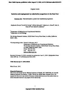
An FSM can be represented by a state transition diagram, a directed graph whose vertices correspond to the states of the machine and whose edges correspond to the state transitions; each edge is labeled with the input and output associated with the transition. For the FSM in Fig. 2.1, suppose that the machine is currently in state s 1 . Upon input b, the machine moves to state s 2 and outputs 1. Equivalently, an FSM can be represented by a state table with one row for each state and one column for each input symbol. For a combination of a present state and input symbol, the corresponding entry in the table specifies the next state and output. For example, Table 2.1 describes the machine in Fig. 2.1. We denote the number of states, inputs, and outputs by n = S , p = I , and q = O , respectively. We extend the transition function δ and output function λ from input symbols to strings as follows: for an initial state s 1 , an input sequence x = a 1 ,... ,a k takes the machine successively to states s i + 1 = δ(s i , a i ), i = 1 , . . . , k, with the final state δ(s 1 , x) = s k + 1 , and produces an output sequence λ(s 1 , x) = b 1 ,... ,b k , where b i = λ(s i , a i ), i = 1 , . . . , k. Suppose that the machine in Fig. 2.1 is in state s 1 . Input sequence abb takes the machine through states s 1 , s 2 , and s 3 , and outputs 011. Also, we can extend the transition and output functions from a single state to a set of states: if Q is a set of states and x an input sequence, then δ(Q,x) = {δ(s,x)  s ∈ Q} 1 , and λ(Q,x) = {λ(s,x)  s ∈ Q}.

________________ 1 We remove the redundant states to make δ(Q, x) a set.

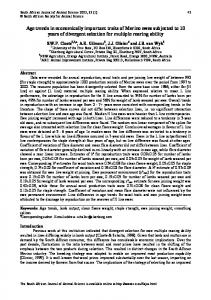
-6An input sequence x induces a partition π(x) on the set of states S of an FSM M, where two states s i , s j are placed in the same block of the partition if and only if they are not distinguished by x, i.e., λ(s i ,x) = λ(s j ,x). This partition is called the initial state uncertainty of x; note that after applying an input sequence x to M and observing the output, the information we acquire about the initial state of M (i.e., the state before the application of x) is the block of π(x) to which it belongs. The information about the current state of M after applying the sequence x is captured by the family of sets: σ(x) = { δ(B,x)  B ∈ π(x) }, called the current state uncertainty of x. Note that σ(x) is not necessarily a partition; i.e., the sets in σ(x) are not necessarily disjoint. The output produced by M in response to the input sequence x tells us to which member of σ(x) the current state belongs. For example, consider the machine M shown in Fig. 2.1 and input b. If we observe output 1, then we know that the machine was initially in state s 1 or s 2 and the current state is s 2 or s 3 ; if we observe output 0, then the initial state was s 3 and the current state is s 1 . Thus, the initial state uncertainty of b is π(b) = {{ s 1 ,s 2 },{ s 3 }} and the current state uncertainty is σ(b) = { {s 2 ,s 3 }, {s 1 } }. The successor tree of a machine is a tree showing the behavior of the machine starting from all possible initial states under all possible input sequences. For every input sequence the tree contains a path starting from the root, and every node is annotated with the corresponding current (and/or initial) state uncertainty. Figure 2.2 shows the successor tree of the machine in Fig. 2.1 for input sequences of length at most 2. Thus for example the root is labeled by the whole set of states, the right child is labeled by σ(b) = { {s 2 ,s 3 }, {s 1 } } with corresponding outputs λ({s 1 , s 2 }, b) = {1} and λ({s 3 }, b) = {0}, and so forth. The transition diagram of an FSM is a directed graph, and thus graph theoretic concepts and algorithms are useful in the analysis of FSM’s. For example, we may want to visit the nodes (states) and edges (transitions), record the order of the visit, and explore the structure of the graph such as its connectivity properties. This can be done by a depth-first-search (DFS) or breadthfirst-search (BFS), resulting in a spanning tree of the graph [AHU, CLR]. We may want to find a shortest path between two nodes [AHU, CLR], constructing a shortest transfer sequence from one state to the other. We may also want to find a path that traverses each edge at least once; it is called a covering path, and we usually want to find one with the minimum number of edges [EJ, Law]. For all these basic concepts, data structures, and graph algorithms, see the references. The finite state machine in Definition 2.1 is fully specified in a sense that at a state and upon an input there is a specified next state by the state transition function and a specified output by the output function. Otherwise, the machine is partially specified; at certain states with some inputs, the next states or outputs are not specified. Also the machine defined is deterministic; at a state and upon an input, the machine follows a unique transition to a next state. Otherwise, the machine is nondeterministic; the machine may follow more than one transition and produce different outputs accordingly. In the applications of protocols, systems can be partially specified and/or nondeterministic

-7-

due to the incomplete specification, unobservable internal transitions, unpredictable behavior of timers and error conditions, etc. Also, testing is usually performed at different levels, and a feature may or may not give rise to nondeterminism depending on whether it is modelled at that level or abstracted away, and depending on whether it is under the control of the tester or not. In the main exposition, we shall focus on fully specified and deterministic machines. We then extend the discussion to partially specified machines in Section 4.7. The theory in these cases is better developed; we now have a reasonably good understanding of the complexity and algorithms for the various problems of interest. For nondeterministic machines, the basic algorithmic theory is not as well developed; we defer the topic to Section 6. 2.1. Machine Equivalence, Isomorphism, and Minimization Two states s i and s j are equivalent if and only if for every input sequence the machine will produce the same output sequence regardless of whether s i or s j is the initial state; i.e., for an arbitrary input sequence x, λ(s i , x) = λ(s j , x). Otherwise, the two states are inequivalent, and there exists an input sequence x such that λ(s i , x) ≠ λ(s j , x); in this case, such an input sequence is called a separating sequence of the two inequivalent states. For two states in different machines with the same input and output sets, equivalence is defined similarly. Two machines M and M′ are equivalent if and only for every state in M there is a corresponding equivalent state in M′, and vice versa. Let M = (I, O, S, δ, λ) and M′ = (I, O, S′, δ ′, λ ′) be two machines with the same input and output sets. A homeomorphism from M to M′ is a mapping φ from S to S′ such that for every state s in S and for every input symbol a in I, it holds that δ ′(φ(s) , a) = φ(δ(s, a) ) and λ ′(φ(s) , a) = λ(s, a). If φ is a bijection, then it is called an isomorphism; clearly in this case M and M′ must have the same number of states and they are identical except for a renaming of states. Two machines are called isomorphic if there is an isomorphism from one to the other. Obviously, two isomorphic FSM’s are equivalent; the converse is not true in general. Machine equivalence is an equivalence relation on all the FSM’s with the same inputs and outputs. In each equivalence class there is a machine with the minimal number of states, called a minimized (reduced) machine. A machine is minimized if and only if no two states are equivalent. In an equivalence class, any two minimized machines have the same number of states; furthermore, there is a one-to-one correspondence between equivalent states, which gives an isomorphism between the two machines. That is, the minimized machine in an equivalence class is unique up to isomorphism. Given an FSM M, we can find its equivalent minimized machine through a state partitioning as follows. State equivalence is an equivalence relation on the set of states, and thus we can partition the states into blocks (classes) of equivalent states. There is a well known algorithm that splits states successively into equivalent blocks [Koh, Mo]. We describe it informally here. We first split states by output symbols: two states are placed in the same block if and only if they

-8-

produce the same output for each input symbol. We then further split repeatedly each block into subblocks according to the transitions: two states are in the same subblock if and only if they are mapped into the same block by each input symbol. This process is repeated until we cannot split anymore. When we terminate, each block contains equivalent states and states in different blocks are inequivalent. In addition, for states in different blocks, a concatenation of input symbols for splitting them apart provides a separating sequence of length no more than n − 1. During a round of splitting, we examine all the p inputs for each of the n states, and there are no more than n − 1 rounds of splitting, since there are n states. Therefore, the total time complexity of a straightforward implementation of this state partitioning is O(pn 2 ). A modification of an algorithm for automata minimization [Hop] gives a fast algorithm with complexity O(pnlog n). After partitioning the states of the machine M into blocks of equivalent states, say r blocks B 1 , ... , B r , we can construct the equivalent minimized machine M′ as follows. We ‘‘project’’ each block into one state: B i → t i , and let the set of states of M′ be S′ = {t i  i = 1 , . . . , r}. To define the state transition function δ ′ and output function λ ′ recall that for every input symbol a all the states of a block B i are mapped to the same block, say B j and produce the same output symbol, say o; then let δ ′(t i , a) = t j and λ ′(t i , a) = o. No two states in M′ are equivalent and we have the minimized machine that is equivalent to M. Note that M′ is a homomorphic image of M (and of all the machines in the equivalence class of M); the homomorphism takes all the equivalent states of a block B i into the corresponding state t i in the minimized machine. There is a range of equivalence relations of states of machines (transition systems in general) from observational to strong bisimulation equivalences [Mi]. For fully specified and deterministic machines as in Definition 2.1, they are the same, and for more general machines such as nondeterministic machines they are different. We shall address this issue later in Section 5 and 6. 2.2. Testing Problems In a testing problem we have a machine M about which we lack some information, and we would like to deduce this information by its I/O behavior; we apply a sequence of input symbols to M, observe the output symbols produced, and infer the needed information of the machine. A test can be preset - if an input sequence is fixed ahead of time - or can be adaptive - if at each step of the test, the next input symbol depends on the previously observed outputs. Adaptive tests are more general than preset tests. Note that an adaptive test is not a test sequence but rather a decision tree. We discuss five fundamental problems. In the first three problems we have a complete description of the machine M = (I, O, S, δ, λ) but we do not know in which state it is; i.e., its initial state. Problem 1. (Homing/Synchronizing Sequence): Determine the final state after the test. Problem 2. (State Identification): Identify the unknown initial state.

-9-

Problem 3. (State Verification): The machine is supposed to be in a particular initial state; verify that it is indeed in that state. In the other two problems the machine M that is being tested is a black box; i.e., we do not know its state diagram (the transition and output function), though we may have some limited information, for example, a bound on the number of states. Problem 4. (Machine Verification/Fault Detection/Conformance Testing): We are given the complete description of another machine A, the ‘‘specification machine’’. Determine whether M is equivalent to A. Problem 5. (Machine Identification): Identify the unknown machine M. For each of these problems the basic questions are the following: Question 1. Existence: Is there a test sequence that solves the problem? Question 2. Length: If it exists, how long does it need to be? Question 3. Algorithms and Complexity: How hard is it to determine whether a sequence exists, to construct one, and to construct a short one? Problem 1 was addressed and essentially solved completely around 1960 using homing and synchronizing sequences; these sequences are described in Section 2.3 and 2.4, respectively. Problems 2 and 3 are solved by distinguishing and UIO sequences, which are the topics of Section 3. For Problem 4, different methods are studied in Section 4. Problem 5 is discussed in Section 7. 2.3. Homing Sequences Often we do not know in which state the machine is, and we want to perform a test, observe the output sequence, and determine the final state of the machine; the corresponding input sequence is called a homing sequence. The homing sequence problem is simple and was completely solved [Koh, Mo]. Only reduced machines have homing sequences, since we cannot distinguish equivalent states using any test. On the other hand, every reduced machine has a homing sequence, and we can construct one easily in polynomial time. First note that an input sequence x is a homing sequence if and only if all the blocks in its current state uncertainty σ(x) are singletons (contain one element). Initially, the machine can be in any one of the states, and thus the uncertainty has only one block S with all the states. We take two arbitrary states in the same block, find a sequence that separates them (it exists because the machine is reduced), apply it to the machine, and partition the current states into at least two blocks, each of which corresponds to a different output sequence. We repeat this process until every block of the current state uncertainty σ(x) contains a single state, at which point the constructed input sequence x is a homing sequence. For example, for the machine in Fig. 2.1, input b separates state s 3 from s 1 (and s 2 ) by their different

- 10 -

outputs 0 and 1, taking states s 1 , s 2 , and s 3 to s 2 , s 3 , and s 1 , respectively. If we have observed output 0, then we know that we are in state s 1 . Otherwise, we have observed output 1 and we could either be in state s 2 or s 3 . We then apply input a to separate s 2 from s 3 by their outputs 1 and 0. Therefore, ba is a homing sequence that takes the machine from states s 1 , s 2 , and s 3 to s 2 , s 3 , and s 1 , respectively; the final state can be determined by the corresponding output sequences 11, 10, and 00, respectively. Observe that after applying input b and observing 0, we know the machine must be in state s 1 , and there is no need to further apply input a; however, if we observe output 1, we have to further input a. Such an adaptive homing sequence can be shorter than preset ones. Since we can construct a separating sequence of length no more than n − 1 for any two states and we apply no more than n − 1 separating sequences before each block of current states contains a singleton state, we concatenate all the separating sequences and obtain a homing sequence of length no more than (n − 1 ) 2 . As a matter of fact, a tight upper bound on the length of homing sequences is n(n − 1 )/2 [Koh, Mo]. On the other hand, a tight lower bound is also n(n − 1 )/2 even if we allow adaptiveness, matching the upper bound; i.e., there exists a machine whose shortest (preset or adaptive) homing sequence is of length at least n(n − 1 )/2 [Koh]. Of course, a given FSM may have a shorter homing sequence than the one constructed by the above algorithm. It is straightforward to find a shortest homing sequence from the successor tree of the machine [Koh, p. 454]; we only need to find a node of least depth d, which is labeled by a current state uncertainty consisting of singletons. For example, a shortest homing sequence of the machine in Fig. 2.1 is ba, using the successor tree in Fig. 2.2. However, it takes exponential time to construct the successor tree up to depth d. In fact, finding a shortest homing sequence is an NP-hard problem and is thus unlikely to have a polynomial time algorithm [Ep]. 2.4. Synchronizing Sequences A synchronizing sequence takes a machine to the same final state, regardless of the initial state or the outputs. That is, an input sequence x is synchronizing if and only if δ(s i ,x) = δ(s j ,x) for all pairs of states s i , s j . Thus, after applying a synchronizing sequence, we know the final state of the machine without even having to observe the output. Clearly, every synchronizing sequence is also a homing sequence, but not conversely. In fact, FSM’s may or may not have synchronizing sequences even when they are minimized. We can determine in polynomial time whether a given FSM has a synchronizing sequence and construct one as follows [Ep, Koh]. Given the transition diagram G of an FSM M, we construct an auxiliary directed graph G×G with n(n + 1 )/2 nodes, one for every unordered pair (s i , s j ) of nodes of G (including pairs (s i , s i ) of identical nodes). There is an edge from (s i , s j ) to (s p , s q ) labeled with an input symbol a if and only if in G there is a transition from s i to s p and a transition from s j to s q , and both are labeled by a. For the machine in Fig. 2.3, the auxiliary graph is shown in Fig. 2.4 (we omit the self-loops). For instance, input a takes the machine from both state s 2 and s 3 to

- 11 -

state s 2 and there is an edge from (s 2 , s 3 ) to (s 2 , s 2 ). It is easy to verify that there is an input sequence that takes the machine from states s i and s j , i ≠ j, to the same state s r if and only if there is a path in G×G from node (s i , s j ) to (s r , s r ). Therefore, if the machine has a synchronizing sequence, then there is a path from every node (s i , s j ), 1 ≤ i < j ≤ n, to some node (s r , s r ), 1 ≤ r ≤ n with equal first and second components. As we will show shortly, the converse is also true; i.e., this reachability condition is necessary and sufficient for the existence of a synchronizing sequence. In Fig. 2.4, node (s 2 , s 2 ) is reachable from nodes (s 1 , s 2 ), (s 1 , s 3 ), and (s 2 , s 3 ), and, therefore, machine in Fig. 2.3 has a synchronizing sequence. In general, the reachability condition can be checked easily using a breadth-first-search [AHU, CLR] in time O(pn 2 ), and, consequently, the existence of synchronizing sequences can be determined in time O(pn 2 ). Suppose that the graph G×G satisfies the reachability condition that there is a path from every node (s i , s j ), 1 ≤ i < j ≤ n, to some node (s r , s r ) We now describe a polynomial time algorithm for constructing a synchronizing sequence. Take two states s i ≠ s j , find a shortest path in G×G from node (s i , s j ) to a node (s r , s r ) ( the path has length no more than n(n − 1 )/2), and denote the input sequence along the path by x 1 . Obviously, δ(s i , x 1 ) = δ(s j , x 1 ) = s r . Also S 1 = δ(S, x 1 ) has no more than n − 1 states. Similarly, we examine S 1 , take two distinct states, apply an input sequence x 2 , which takes them into the same state, and obtain a set of current states S 2 of no more than n − 2 states. We repeat the process until we have a singleton current state S k = {s t }; this is always possible because G×G satisfies the reachability condition. The concatenation x of input sequences x 1 , x 2 , . . . , x k takes all states into state s t , and x is a synchronizing sequence. In Fig. 2.4, node (s 2 , s 2 ) is reachable from (s 2 , s 3 ) via the input a which takes the machine to state s 1 (if it starts in s 1 ) and s 2 (if it starts in s 2 or s 3 ). Therefore, we have S 1 = {s 1 , s 2 } = δ(S, a). Since node (s 2 , s 2 ) is reachable from (s 1 , s 2 ), the input sequence ba takes the machine to state s 2 if it starts in s 1 or s 2 , and we have S 2 = {s 2 } = δ(S 1 , ba). Therefore, we obtain a synchronizing sequence aba by concatenating input sequences a and ba, with δ(S, aba) = {s 2 }. Since the number of times we merge pairs of states is at most n − 1 and the length of each merging sequence is x i  ≤ n(n − 1 )/2, the length of synchronizing sequences is no more than n(n − 1 ) 2 /2. The algorithm can be implemented to run in time O(n 3 + pn 2 ) [Ep]. If in each stage we choose among the pairs of current states that pair which has the shortest path to a node of the form (s r ,s r ), then it can be shown by a more careful argument that the length of the constructed synchronizing sequence is at most n(n 2 − 1 )/6 [Koh]. The best known lower bound is (n − 1 ) 2 ; i.e., there are machines that have synchronizing sequences and the shortest such sequences have length (n − 1 ) 2 . There is a gap between this quadratic lower bound and the cubic upper bound; closing this gap remains an open problem. For a given machine, we can find a shortest synchronizing sequence using a successor tree. For this purpose we only need to label each node of the tree with the set of current states; i.e., if a

- 12 node v corresponds to input sequence x then we label the node with δ(S,x). A node of least depth d whose label is a singleton corresponds to a shortest synchronizing sequence. It takes exponential time to construct the successor tree up to depth d to find such a node and the shortest sequence. In fact, finding the shortest synchronizing sequence is an NP-hard problem [Ep].

3. STATE IDENTIFICATION AND VERIFICATION We now discuss testing Problems 2 and 3: state identification and verification. We want to determine the initial state of a machine before a test instead of the final state after a test as in Problem 1. The problems become harder; while running a test to deduce needed information, we may also introduce ambiguity and we may lose the initial state information irrevocably. Problem 2. State Identification. We know the complete state diagram of a machine M but we do not know its initial state. The problem is to identify the unknown initial state of M. This is not always possible, i.e., there are machines M for which there exists no test that will allow us to identify the initial state. An input sequence that solves this problem (if it exists) is called a distinguishing sequence [G1, G2, Koh]. Note that a homing sequence solves a superficially related but different problem: to perform a test after which we can determine the final state of the machine. Every distinguishing sequence also provides a homing sequence; once we know the initial state we can trace down the final state. However, the converse is not true in general. Problem 3. State Verification. Again we know the state diagram of a machine M but not its initial state. The machine is supposed to be in a particular initial state s 1 ; verify that it is in that state. Again, this is not always possible. A test sequence that solves this problem (if it exists) is called a Unique Input Output sequence for state s 1 (UIO sequence, for short) [SD]. This concept has been reintroduced at different times under different names; for example, it is called ‘‘simple I/O sequence’’ in [Hs] and ‘‘checkword’’ in [Gob]. Distinguishing sequences and UIO sequences are interesting in their own right in offering a solution to the state identification and verification problems, respectively. Besides, these sequences have been useful in the development of techniques to solve another important problem: conformance testing. See Section 4. There is an extensive literature on these two problems starting with Moore’s seminal 1956 paper on ‘‘gedanken-experiments’’ [Mo] where the notion of distinguishing experiment was first introduced. Following this work, several papers were published in the 60’s on state identification motivated mainly by automata theory and testing of switching circuits [G1, G2, KK, Koh]. The state verification problem was studied in early 70’s [Gob, Hs]. However, only exponential algorithms were given for state identification and verification, using successor trees. Sokolovskii [So] first proved that if a machine has an adaptive distinguishing sequence, then there is one of polynomial length. However, he only gave an existence proof and did not provide efficient algorithms for determining the existence of and for constructing distinguishing sequences. In the last few

- 13 -

years there has been a resurgence of activities on this topic motivated mainly by conformance testing of communication protocols [ADLU, CZ, DSU, Gon, KSNM, MP1, SL1, SL2]. Consequently, the problems of state identification and verification have resurfaced. The complexity of state identification and verification has been resolved recently [LY1] as follows. The preset distinguishing sequence and the UIO sequence problems are both PSPACEcomplete. Furthermore, there are machines that have such sequences but only of exponential length. Surprisingly, for the adaptive distinguishing sequence problem, there are polynomial time algorithms that determine the existence of adaptive distinguishing sequences and construct such a sequence if it exists. Furthermore, the sequence constructed has length at most n(n − 1 )/2, which matches the known lower bound. 3.1. Preset Distinguishing Sequences Recall that a test can be preset - if an input sequence is fixed ahead of time - or can be adaptive - if at each step of the test, the next input symbol depends on the previously observed outputs. Adaptive tests are more general than preset tests and an adaptive test is not a test sequence but rather a decision tree. Given a machine M, we want to identify its unknown initial state. This is possible if and only if the machine has a distinguishing sequence [G1, G2, Koh]. We discuss preset test first: Definition 3.1. A preset distinguishing sequence for a machine is an input sequence x such that the output sequence produced by the machine in response to x is different for each initial state, i.e.; λ(s i , x) ≠ λ(s j , x) for every pair of states s i , s j , i ≠ j.

For example, for the machine in Fig. 2.1, ab is a distinguishing sequence, since λ(s 1 , ab) = 01, λ(s 2 , ab) = 11, and λ(s 3 , ab) = 00. Clearly, an FSM that is not reduced cannot have a distinguishing sequence since equivalent states can not be distinguished from each other by tests. We only consider reduced machines. However, not every reduced machine has a distinguishing sequence. For example, consider the FSM in Fig. 3.1. It is reduced: the input b separates state s 1 from states s 2 and s 3 , and input a separates s 2 from s 3 . However, there is no single sequence x that distinguishes all the states simultaneously: a distinguishing sequence x cannot start with letter a because then we would never be able to tell whether the machine started in state s 1 or s 2 , since both these states produce the same output 0, and make a transition to the same state s 1 . Similarly, the sequence cannot start with b because then it would not be able to distinguish s 2 from s 3 . Thus, this machine does not have any distinguishing sequence. It is not always as easy to tell whether an FSM has a distinguishing sequence. The classical

- 14 -

algorithm found in textbooks [G1, G2, Koh] works by examining a type of successor tree (called a distinguishing tree) whose depth is equal to the length of the distinguishing sequence (which is no more than exponential [Koh]). For this purpose we need to annotate the nodes of the successor tree with the initial state uncertainty. Note that a sequence x is a distinguishing sequence if and only if all blocks of its initial state uncertainty π(x) are singletons. The classical algorithms using successor trees take at least exponential time. This is probably unavoidable in view of the following result: It is PSPACE-complete to test whether a given FSM has a preset distinguishing sequence. This holds even when machines are restricted to have only binary input and output alphabets. Furthermore, there are machines for which the shortest preset distinguishing sequence has exponential length. For detailed proofs see [LY1]. Therefore, preset tests for state identification, if they exist, may be inherently exponential. However, for adaptive testing we have polynomial time algorithms; such a test is provided by an adaptive distinguishing sequence. 3.2. Adaptive Distinguishing Sequences An adaptive distinguishing sequence is not really a sequence but a decision tree: Definition 3.2. An adaptive distinguishing sequence is a rooted tree T with exactly n leaves; the internal nodes are labeled with input symbols, the edges are labeled with output symbols, and the leaves are labeled with states of the FSM such that: (1) edges emanating from a common node have distinct output symbols, and (2) for every leaf of T, if x, y are the input and output strings respectively formed by the node and edge labels on the path from the root to the leaf, and if the leaf is labeled by state s i of the FSM then y = λ(s i ,x). The length of the sequence is the depth of the tree.

In Fig. 3.3 we show an adaptive distinguishing sequence for the FSM in Fig. 3.2. The adaptive experiment starts by applying input symbol a, and then splits into two cases according to the observed output 0 or 1, corresponding to the two branches of the tree. In the first case we apply a, then b followed by a, and split again into two subcases depending on the last output. If the last output is 0, then we declare the initial state to be s 5 ; otherwise, we apply ba and depending on the observed output, we declare the initial state to be s 1 or s 3 . We carry out the experiment analogously in case we fall in the right branch of the tree. Not all reduced FSM’s have adaptive distinguishing sequences. For example, the FSM in Fig. 3.1 does not have any (for the same reason as in the preset case). Of course, a preset distinguishing sequence is also an adaptive one. Thus, machines with preset distinguishing sequences have also adaptive ones, and furthermore the adaptive ones can be much shorter. On the other hand, an FSM may have no preset distinguishing sequences but still have an adaptive one. The machine in Fig. 3.2 is such an example. A preset distinguishing sequence for this machine can only start with a because b merges states s 1 , s 2 and s 6 without distinguishing them. After

- 15 -

applying a string of a’s, both the initial and the current state uncertainty are τ = { {s 1 ,s 3 ,s 5 } , {s 2 ,s 4 ,s 6 } }, and, therefore, b can never be applied because it merges s 2 and s 6 without distinguishing them. Sokolovskii showed that if an FSM has an adaptive distinguishing sequence, then it has one π2 of length ___ n 2 , and this is the best possible up to a constant factor in the sense that there are 12 FSM’s whose shortest adaptive distinguishing sequence has length n(n − 1 )/2 [So]. His proof of the upper bound is not constructive and does not suggest an algorithm; he argues basically that if one is given a sequence that is too long then there exists a shorter one. This result implies that the existence question is in NP. The classical approach for constructing adaptive distinguishing sequences [G1, G2, Koh] is again a semienumerative type of algorithm that takes exponential time. The algorithm is naturally more complicated than the one for the preset case, which probably accounts for the belief that one of the ‘‘main disadvantages of using adaptive experiments (for state identification) is the relative difficulty in designing them’’ [Koh]. A polynomial time algorithm was recently found [LY1]. We will describe next the algorithm for determining the existence of an adaptive distinguishing sequence, and in the next subsection we will describe the algorithm for constructing one. Consider an adaptive experiment (not necessarily a complete adaptive distinguishing sequence). The experiment can be viewed as a decision tree T whose internal nodes are labeled with input symbols and the edges with output symbols. With every node u of T we can associate two sets of states, the initial set I(u) and the current set C(u). If x and y are respectively the input and output strings formed by the labels on the path from the root to node u (excluding u itself), then I(u) = { s i ∈ S  y = λ(s i , x) } (the set of initial states that will lead to node u), and C(u) = { δ(s i , x)  s i ∈ I(u) } (the set of possible current states after this portion of the experiment). The initial sets I(u) associated with the leaves u of T form a partition π(T) of the set of states of the machine (every initial state leads to a unique leaf of the decision tree), which represents the amount of information we derive from the experiment. The experiment T is an adaptive distinguishing sequence if and only if π(T) is the discrete partition: all blocks are singletons. Note that the current sets associated with the leaves need not be disjoint. We say that an input a (or more generally an input sequence) is valid for a set of states C if it does not merge any two states s i , s j of C without distinguishing them, i.e., either λ(s i ,a) ≠ λ(s j ,a) or δ(s i ,a) ≠ δ(s j ,a). If during the test we apply an input a such that λ(s i ,a) = λ(s j ,a) and δ(s i ,a) = δ(s j ,a) for two states s i , s j of the current set, then we lose information irrevocably, because we will never be able to tell whether the machine was in state s i or s j . Therefore, an adaptive distinguishing sequence can apply in each step only inputs that are valid for the current set. The difference between the preset and adaptive case is that in the preset case we have to worry about validity with respect to a collection of sets (the current state uncertainty), whereas in the adaptive case we only need validity with respect to a single set, the current

- 16 -

set under consideration. The algorithm for determining whether there exists an adaptive distinguishing sequence is rather simple. It maintains a partition π of the set of states S; this should be thought of as a partition of the initial states that can be distinguished. We initialize the partition π with only one block containing all the states. While there is a block B of the current partition π and a valid input symbol a for B, such that two states of B produce different outputs on a or move to states in different blocks, then refine the partition: replace B by a set of new blocks, where two states of B are assigned to the same block in the new partition if and only if they produce the same output on a and move to states of the same block (of the old partition). It was shown in [LY1] that the machine has an adaptive distinguishing sequence if and only if the final partition is the discrete partition. Consider the machine of Fig. 3.2. Initially the partition π has one block S with all the states. Input symbol b is not valid, but a is. Thus, π is refined to π 1 = { {s 1 ,s 3 ,s 5 } , {s 2 ,s 4 ,s 6 } }. Now b is valid for the first block of π 1 which it can refine because s 1 stays under b in the same block, whereas s 3 and s 5 move to the second block. Thus, the new partition is π 2 = { {s 1 } , {s 3 ,s 5 } , {s 2 ,s 4 ,s 6 } }. Next, input a can refine the block {s 2 ,s 4 ,s 6 } into {s 2 ,s 4 }, {s 6 }. After this, b becomes valid for {s 3 ,s 5 } which it refines to {s 3 }, {s 5 }. Finally, either a or b can refine the block {s 2 ,s 4 } into singletons ending with a discrete partition, and thus the machine has an adaptive distinguishing sequence. The decision algorithm is very similar to the classical minimization algorithm. The major difference is that only valid inputs can be used to split blocks, A straightforward implementation of the algorithm, as we have described it, takes time O(pn 2 ). It was shown in [LY1] how to implement the algorithm so that it runs in time O(pnlog n).

3.3. Constructing Adaptive Distinguishing Sequences The algorithm for constructing an adaptive distinguishing sequence is somewhat more complicated so that polynomial time of construction and polynomial length of the constructed sequence can be ensured. The basic ideas are: (1) We perform the splitting conservatively, one step at a time, and (2) We split the blocks in a particular order, namely, split simultaneously all blocks of largest cardinality before going on to the smaller ones. We present the construction in two steps as follows. Algorithm 3.1 does the partition refinement and constructs a tree, which we call a splitting tree, that reflects the sequence of block splittings. Algorithm 3.2 constructs an adaptive distinguishing sequence from the splitting tree. We present the algorithms and explain by examples. For details see [LY1]. The splitting tree is a rooted tree T. Every node of the tree is labeled by a set of states; the root is labeled with the whole set of states, and the label of an internal (nonleaf) node is the union of its children’s labels. Thus, the leaf labels form a partition π(T) of the set of states of the

- 17 -

machine M, which should be thought of as a partition of the initial states. The splitting tree is complete if the partition is a discrete partition. In addition to the set-labels, we associate an input string ρ with every internal node u. Every edge of the splitting tree is labeled by an output symbol. In the algorithm below we use the notation δ − 1 (Q, σ) for a set Q of states and an input sequence σ to denote the set of states s ∈ S for which δ(s, σ) ∈ Q. For a block Q in the current partition π, a valid input a can be classified into one of three types. (i) Two or more states of Q produce different outputs on input a. (ii) All states of Q produce the same output, but they are mapped to more than one block of π. (iii) Neither of the above; i.e., all states produce the same output and are mapped into a same block of π. Define the implication graph of π, denoted G π , to be a directed graph with the blocks of π as its nodes and arcs between blocks with the same number of states as follows. There is an arc B 1 → B 2 labeled by an input symbol a and output symbol o if a is a valid input of type (iii) for B 1 and maps its states one-to-one and onto B 2 with output o. Algorithm 3.1. (Splitting Tree) Input: A reduced FSM M. Output: A complete splitting tree ST if M has an adaptive distinguishing sequence. Method: 1. Initialize ST to be a tree with a single node, the root, labeled with the set S of all the states, and the current partition π to be the trivial one. 2. While π is not the discrete partition do the following. Let R be the set of blocks with the largest cardinality. Let G π be the implication graph of π and G π [R] its subgraph induced by R. For each block B of R, let u(B) be the leaf of the current tree ST with label B. We expand ST as follows. Case (i). If there is a valid input a of type (i) for B, then associate the symbol a with node u(B). For each subset of states of B that produces the same output symbol on input a attach to u(B) a leaf child with this subset as its label; the edge is labeled by the output symbol. Case (ii). Otherwise, if there is a valid input a of type (ii) for B with respect to π, then let v be the lowest node of ST whose label contains the set δ(B,a) (note: v is not a leaf). If the string associated with v is σ, then associate with node u(B) the string aσ. For each child of v whose label Q intersects δ(B,a), attach to u(B) a leaf child with label B∩ δ − 1 (Q,a); the edge incident to u(B) is given the same label as the corresponding edge of v. Case (iii). Otherwise, search for a path in G π from B to a block C that has fallen under Case (i) or (ii). If no such path exists, then we terminate and declare failure (the FSM does not have any adaptive distinguishing sequences); else let σ be the label of (a shortest) such path. By now, u(C) has already acquired children and has been associated with a string τ by the previous cases. Expand the tree as in Case (ii): Associate with u(B) the string σ τ. For each child of u(C) whose label Q intersects δ(B, σ), attach to u(B) a leaf child with label B∩ δ − 1 (Q, σ); the edge incident to u(B) is given the same label as the corresponding edge of u(C).

- 18 -

Example 3.1. Consider the FSM in Fig. 3.2. The splitting tree is shown in Fig. 3.4. We have indexed the internal nodes according to the order in which they are created by Algorithm 3.1, and we have attached the set-labels and the associated strings; we have omitted the edge labels. The only valid input for the set S is a which splits S into two blocks of three states each. Both blocks are considered in the next iteration. The block of node u 1 has a valid input of type (ii), namely b, which maps it into the root block, and thus node u 1 gets the string ba and acquires two children. The block of node u 2 has only a valid input of type (iii), namely a, which gives a path of length 1 in the implication graph to the block of u 1 ; thus, u 2 gets the string aba. In the next iteration we examine the blocks of nodes u 3 and u 4 . Both inputs are valid of type (ii) for u 3 ; we have chosen arbitrarily input a in the figure, so the string of u 3 is a followed by the string of u 2 . The block of u 4 has only valid type (iii) inputs a and b, and both map u 4 into u 3 . We choose b and the string of u 4 is b followed by that of u 3 , i.e., baaba.

It can be shown [LY1] that Algorithm 3.1 succeeds in constructing a complete splitting tree if and only if the FSM has an adaptive distinguishing sequence. The time complexity of the algorithm is O(pn 2 ) and the size of the output of the algorithm, i.e., of the annotated complete splitting tree, is O(n 2 ). We now derive an adaptive experiment for determining the initial state of the FSM, given a complete splitting tree. At each stage, depending on the output seen so far, there is a set I of possible initial states and a set C (of equal size) of the possible current states. The experiment is based on the current states. Algorithm 3.2. (Adaptive Distinguishing Sequence) Input: A complete splitting tree ST. Output: An adaptive distinguishing sequence. Method: Let I, C be the possible initial and current sets that are consistent with the observed outputs (initially, I = C is the whole set S of states). While I > 1 (and thus, also C> 1), find the lowest node u of the splitting tree whose label contains the current set C, apply the input string τ associated with node u, and update I and C according to the observed output.

Example 3.2. Consider again the FSM of Fig. 3.2. If we apply Algorithm 3.2 to the splitting tree ST of Fig. 3.4, we obtain the adaptive distinguishing sequence in Fig. 3.3. First, we input symbol a, the label of the root of ST. Suppose the output is 0. Then the initial set I is {s 1 ,s 3 ,s 5 }, which means that the current set C is {s 2 ,s 4 ,s 6 }. The lowest node of ST that contains C is u 2 , so we apply the input sequence from u 2 : aba. Suppose that the last output is 1. Then the initial set becomes I = {s 1 ,s 3 }, with corresponding current set C = {s 5 ,s 1 }. The lowest node of ST that contains this set is u 1 , so we apply now the sequence from u 1 : ba, after

- 19 -

which we know the initial state. The other branches of the adaptive distinguishing sequence are constructed similarly.

Suppose that Algorithm 3.1 succeeds in constructing a complete splitting tree. Then it can be shown [LY1] that the experiment derived by Algorithm 3.2 identifies correctly the initial state and has length at most n(n − 1 )/2. The adaptive distinguishing sequence (decision tree) has O(n 2 ) nodes and can be constructed in time O(n 2 ) from the splitting tree. The length of the adaptive experiment is tight; there are machines for which the shortest adaptive distinguishing sequence has length n(n − 1 )/2 [So]. Recall that it is hard to determine whether an FSM has a preset distinguishing sequence, and even if such a sequence exists it may be exponentially long. On the other hand, there are efficient algorithms to determine the existence of and to construct adaptive distinguishing sequences that are more general but are shorter than preset ones. Therefore, for state identification problem and for applications such as fault detection (see Section 4), we only have to consider adaptive distinguishing sequences. 3.4. State Verification We now turn to Problem 3. We want to verify that a given machine M with a known state diagram is in a particular state. This is possible if and only if that state has a Unique Input Output (UIO) sequence [Gob, Hs, SD]. Adaptiveness does not make a difference in this case. Definition 3.3. A UIO sequence of a state s is an input sequence x, such that the output sequence produced by the machine in response to x from any state other than s is different than that from s, i.e., λ(s i , x) ≠ λ(s, x) for any s i ≠ s.

An input sequence x is a UIO sequence for a state s if and only if its initial state uncertainty π(x) has s in a singleton block {s}. For example, for the FSM in Fig. 3.1, b is a UIO sequence for state s 1 because it outputs 0 while s 2 and s 3 output 1; state s 2 has no UIO sequence and s 3 has a UIO sequence a. If a machine has a preset or even an adaptive distinguishing sequence, then all states have UIO sequences. More specifically, if a tree T is an adaptive distinguishing sequence, then the input string formed by the node labels on the path from the root to a leaf that declares the initial state to be s i is a UIO sequence for state s i . The converse is not true in general. On the other hand, for a given machine, it is possible that no state has a UIO sequence, that some states have UIO sequences and some do not, or that every state has UIO sequences but there is no adaptive distinguishing sequence. There have been many papers in the last few years, which propose methods for the

- 20 -

conformance testing of protocols based on UIO sequences ([ADLU, CCK, CVI1, CA1, SLD, SSLS, YU] and others). However, no efficient algorithms are known for finding UIO sequences; the proposed methods are based on appropriate successor trees and take exponential time. It turns out that finding UIO sequences is a hard problem [LY1]. For a given machine M, the following three problems are PSPACE-complete. (1) Does a specific given state s of M have a UIO sequence? (2) Do all states of M have UIO sequences? (3) Are there some states of M with UIO sequences. These results hold even in the case of machines with binary input and output alphabets. Furthermore, there are machines whose states have UIO sequences, but only of exponential length. Note that these are worst case results. It has been reported in practical applications that in many cases there exist short UIO sequences, especially in communication protocol machines [ADLU, SD]. 3.5. Remarks In this section we addressed two fundamental problems of testing finite state machines: distinguishing sequences and UIO sequences. These problems and concepts have been around for decades since the pioneering works of Moore and Hennie [He, Mo]. Yet the problems about their existence, length, and complexity of their computation have been resolved only recently [LY1]. We now comment on the relation between these test sequences, since it could be rather confusing. Distinguishing sequences identify the initial state of a machine, whereas UIO sequences solve an easier problem; they only verify if the machine is in a particular initial state. If a finite state machine has a preset distinguishing sequence, then it must have an adaptive one with length no more than n(n − 1 )/2, but not vice versa; there are machines that have adaptive distinguishing sequences but do not have any preset ones. Therefore, for state identification and its applications to fault detection, we would consider adaptive distinguishing sequences. If a machine has an adaptive distinguishing sequence (a decision tree), then each state has a UIO sequence. More specifically, the input sequence from the root of the decision tree to a leaf node, which corresponds to a state, is a UIO sequence for that state and has length no more than n(n − 1 )/2. Therefore, for state verification and its applications to fault detection, we might want to first try adaptive distinguishing sequences to derive UIO sequences; they are short and it takes only polynomial time. In case the machine does not have any adaptive distinguishing sequences, we may try to construct UIO sequences directly. There are machines, which do not have any adaptive distinguishing sequences but do have UIO sequences for some or all states. Note that there is no need to consider ‘‘adaptive’’ UIO sequences; they can always be made preset.

- 21 -

4. CONFORMANCE TESTING We now discuss Problem 4: the conformance testing or fault detection problem. We have complete information of a specification machine A; we have its state transition and output functions in a form of a transition diagram or state table. We are also given an implementation machine B that is a ‘‘black box’’ and we can only observe its I/O behavior. We want to design a test to determine whether B is a correct implementation of A by applying the test sequence to B and observing the outputs. This problem has been referred to as the ‘‘fault detection’’ or ‘‘machine verification’’ problem in the circuits and switching systems literature, and is called the ‘‘conformance testing’’ (or simply ‘‘test generation’’) problem in the literature on communication protocols. 4.1. Preliminaries We wish to test whether an implementation machine B conforms (is equivalent) to the specification machine A. Obviously, without any assumptions the problem is impossible; for any test sequence we can easily construct a machine B, which is not equivalent to A but produces the same outputs as A for the given test sequence. There is a number of natural assumptions that are usually made in the literature in order for the test to be at all possible: Assumption 4.1. (1) Specification machine A is strongly connected; (2) Machine A is reduced; (3) Implementation machine B does not change during the experiment and has the same input alphabet as A; and (4) Machine B has no more states than A.

An FSM is strongly connected if its transition diagram is strongly connected; that is, for every pair of states s i and s j there is an input sequence x that takes the machine from state s i to s j : δ(s i ,x) = s j . The reason for Assumption (1) is that, if A is not strongly connected, and if in the experiment the machine B starts at a state that cannot reach some other states, then in the test we will not be able to visit all states of the machine, thus, we will not be able to tell with certainty whether B is correct. The rationale for Assumption (2) is that we can always minimize A if it is not reduced, and anyway by testing B we can only determine it up to equivalence because all equivalent machines have the same I/O behavior. The reason for Assumption (3) is obvious. In addition, an upper bound must be placed on the number of states of B; otherwise, no matter how long our test is, it is possible that it does not reach the ‘‘bad’’ part of B. The usual assumption made in the literature, and which we will also adopt for most of this section, is Assumption (4): the faults do not increase the number of states of the machine. In other words, under this assumption, the faults are of two types: ‘‘output faults’’; i.e., one or more transitions may produce wrong outputs, and ‘‘transfer faults’’; i.e., transitions may go to wrong next states. However, in applications such as protocol testing, implementation machines may have more states than that of the specification machines. The additional difficulties due to extra states are

- 22 -

orthogonal to the checking problem itself; We will discuss later in Section 4.7.2 what happens when assumption (4) is relaxed; the additional difficulties due to extra states are orthogonal to the checking problem itself. Under these assumptions, we want to design an experiment that tests whether B is equivalent to A. The following fact is easy to prove, and is well known [Koh, Mo]. Proposition 4.1. Let A and B be two FSM’s satisfying Assumption 4.1. The following are equivalent: (1) A and B are isomorphic; (2) A and B are equivalent; and (3) At least one state of A has an equivalent state in B.

Note that our notion of a specification FSM does not include an initial state. If the specification A includes also a designated initial state s 1 that has to be verified, then a test may not exist, since this is a state verification problem, see Section 3.4. On the other hand, suppose that the implementation machine B starts from an unknown state and that we want to check whether it is isomorphic to A. We first apply a homing sequence that is supposed to bring B (if it is correct) to a known state s 1 that is the initial state for the main part of the test, which is called a checking experiment and accomplishes the following. If B is isomorphic to A, then the homing sequence has brought B to the initial state s 1 and then the checking experiment will verify that B is isomorphic to A. However, if B is not isomorphic to A, then the homing sequence may or may not bring B to s 1 ; in either case, a checking experiment will detect faults: a discrepancy between the outputs from B and the expected outputs from A will be observed. From now on we assume that a homing sequence has taken the implementation machine B to a supposedly initial state s 1 before we conduct a conformance test. Definition 4.1. Let A be a specification FSM with n states and initial state s 1 . A checking sequence for A is an input sequence x that distinguishes A from all other machines with n states; i.e., every (implementation) machine B with at most n states that is not isomorphic to A produces on input x a different output than that produced by A starting from s 1 .

All the proposed methods for checking experiments have the same basic structure. We want to make sure that every transition of the specification FSM A is correctly implemented in FSM B; so for every transition of A, say from state s i to state s j on input a, we want to apply an input sequence that transfers the machine to s i , apply input a, and then verify that the end state is s j by applying appropriate inputs. The methods differ by the types of subsequences they use to verify that the machine is in a right state. This can be accomplished by status messages, separating family of sequences, distinguishing sequences, UIO sequences, characterizing sequences, and identifying sequences. Furthermore, these sequences can be selected deterministically or randomly.

- 23 -

These methods will be surveyed in this section. We introduce some basic concepts first. A separating family of sequences for A is a collection of n sets Z i , i = 1 ,... ,n, of sequences (one set for each state) such that for every pair of states s i , s j there is an input string α that (1) separates them, i.e., λ A (s i ,α) ≠ λ A (s j ,α) (where λ A is the output function of A), and (2) α is a prefix of some sequence in Z i and some sequence in Z j . We call Z i the separating set of state s i , and the elements of Z i its separating sequences. There are many ways for choosing separating sets for an FSM. If the machine A has a preset distinguishing sequence x, then we may choose all the Z i ’s to be {x}. If A has an adaptive distinguishing sequence, then we may choose Z i to have a single element, namely the input sequence for which the adaptive distinguishing experiment declares the initial state to be s i (i.e., the input sequence that labels the path from the root to the leaf labeled s i ). In fact, it is not hard to see that we can satisfy the separation property with all sets Z i being singletons if and only if A has an adaptive distinguishing sequence. However, even if every state s i has a UIO sequence x i , we may not be able to choose the singletons {x i } as separating sets, because they may violate the prefix condition of the separation property. Every reduced machine has a separating family. One way of constructing a separating family for a general reduced machine A is as follows. Since the specification machine A is reduced, we can find a separating sequence x for any two distinct states s i and s j , using the method in Section 2.1. We then partition the states into blocks based on their different outputs λ(s k , x), k = 1 , . . . , n; each state s k takes x as a separating sequence in its set Z k . Then for each block with more than one state, we repeat the process until each block becomes a singleton set. The resulting family of sets has the property that, for every pair of states s i , s j their corresponding sets Z i , Z j contain a common sequence that separates them; therefore it is a separating family. There are no more than n − 1 partitions and each Z i has no more than n − 1 separating sequences. According to this procedure, the sets Z i for different states s i could be different because the states are involved in different splittings and we need to include a sequence in Z i only if s i is involved in the splitting. If instead we let every Z i include the separating sequence for every splitting of every block, no matter whether the corresponding state s i is involved in the splitting or not, then all the Z i ’s would be identical and still each of them would have no more than n − 1 sequences of length less than n. Such a set of sequences is called a set of characterizing sequences [He, Koh]; any two states are separable by a sequence in the set. Note that we want the Z i ’s to contain as few and as short sequences as possible. We allow the sets Z i for different states to be different, instead of an identical characterizing set, for two reasons. First, because this allows more flexibility, thus we may be able to use smaller sets with shorter sequences and thus shorten the conformance test. Second, this is needed for the test to generalize to partially specified machines, because in this case, there may even not exist a set of characterizing sequences that is defined for all the states. We say that a state q i of B is similar to state s i of A if it agrees (gives the same output) on

- 24 -

all sequences in the separating set Z i of s i . The key property is that q i can be similar to at most one state of A. To see this, suppose that q i is similar to states s i and s j and consider a string α that separates s i from s j and is a prefix of sequences in Z i and Z j . Since s i and s j produce different outputs on input α, state q i cannot agree with both, say it disagrees with s i . Then q disagrees with s i on the sequence of Z i that has α as a prefix. Let us say that an FSM B is similar to A, if for each state s i of A, the machine B has a corresponding state q i similar to it. Note that then all the q i ’s must be distinct, and since B has at most n states, there is a one-to-one correspondence between similar states of A and B. In the remainder of this section, we describe different checking experiments. For clarity, we denote the specification and implementation machine by A = (I, O, S A , δ A , λ A ) and B = (I, O, S B , δ B , λ B ), respectively. Furthermore, we assume that B is supposed to be taken by a homing sequence to an initial state, which corresponds to state s 1 of A. 4.2. Status Messages and Reset A status message tells us the current state of a machine. Conceptually, we can imagine that there is a special input status, and upon receiving this input, the machine outputs its current state and stays there. Such status messages do exist in practice. In hardware testing, one might be able to observe register contents which store the states of a sequential circuit, and in protocol testing, one might be able to dump and observe variable values which represent the states of a protocol machine. With a status message, the machine is highly observable at any moment. We say that the status message is reliable if it is guaranteed to work reliably in the implementation machine B; i.e., it outputs the current state without changing it. Suppose the status message is reliable. Then a checking sequence can be easily obtained by simply constructing a covering path of the transition diagram of the specification machine A, and applying the status message at each state visited. Since each state is checked with its status message, we verify whether B is similar to A. Furthermore, every transition is tested because its output is observed explicitly, and its start and end state are verified by their status messages; thus such a covering path provides a checking sequence. If the status message is not reliable, then we can still obtain a checking sequence by applying the status message twice in a row for each state s i at some point during the experiment when the covering path visits s i ; we only need to have this double application of the status message once for each state and have a single application in the rest of the visits. The double application of the status message ensures that it works properly for every state. For example, consider the specification machine A in Fig. 2.1, starting at state s 1 . We have a covering path from input sequence x = ababab. Let s denote the status message. If it is reliable, then we obtain the checking sequence sasbsasbsasbs. If it is unreliable, then we have the sequence ssasbssasbssasbs.

- 25 -

We say that machine A has a reset capability if there is an initial state s 1 and an input symbol r that takes the machine from any state back to s 1 , i.e., δ A (s i , r) = s 1 for all states s i .

2

We

say that the reset is reliable if it is guaranteed to work properly in the implementation machine B, i.e., δ B (s i ,r) = s 1 for all s i ; otherwise it is unreliable. For machines with a reliable reset, there is a polynomial time algorithm for constructing a checking sequence [Ch, CVI1, Vas]. Let Z i , i = 1 ,... ,n be a family of separating sets; as a special case the sets could all be identical (i.e., a characterizing set). We first construct a breadth-firstsearch tree (or any spanning tree) of the transition diagram of the specification machine A and verify that B is similar to A; we check states according to the breadth-first-search order and tree edges (transitions) leading to the nodes (states). For every state s i , we have a part of the checking sequence that does the following for every member of Z i : first it resets the machine to s 1 by input r, then it applies the input sequence (say p i ) corresponding to the path of the tree from the root s 1 to s i and then applies a separating sequence in Z i . If the implementation machine B passes this test for all members of Z i , then we know that it has a state similar to s i , namely the state that is obtained by applying the input sequence p i starting from the reset state s 1 . If B passes this test for all states s i , then we know that B is similar to A. This portion of the test also verifies all the transitions of the tree. Finally, we check nontree transitions. For every transition, say from state s i to state s j on input a, we do the following for every member of Z j : reset the machine, apply the input sequence p i taking it to the start node s i of the transition along tree edges, apply the input a of the transition, and then apply a separating sequence in Z j . If the implementation machine B passes this test for all members of Z j then we know that the transition on input a of the state of B that is similar to s i gives the correct output and goes to the state that is similar to state s j . If B passes the test for all the transitions, then we can conclude that it is isomorphic to A. Example 4.1. For the machine in Fig. 2.1, a family of separating sets is: Z 1 ={ a, b }, Z 2 ={ a }, and Z 3 ={ a, b }. A spanning tree is shown in Fig. 4.1 with thick tree edges. Sequences ra and rb verify state s 1 . Sequence rba verifies state s 2 and transition (s 1 , s 2 ): after resetting, input b verifies the tree edge transition from s 1 to s 2 and separating sequence a of Z 2 verifies the end state s 2 . The following two sequences verify state s 3 and the tree edge transition from s 2 to s 3 : rbba and rbbb where the prefix rbb resets the machine to s 1 and takes it to state s 3 along verified tree edges, and the two suffixes a and b are the separating sequences of s 3 . Finally, we test nontree edges in the same way. For instance, the self-loop at s 2 is checked by the sequence rbaa. ________________ 2 There is occasionally some confusion in the literature concerning the strong connectivity of machine A with a reset. The reset counts also as an input symbol, i.e., if A has a reset symbol and the state s 1 can reach all the other states, then A is considered to be strongly connected (even though the subgraph induced by the transitions on the rest of the input symbols may not be strongly connected).

- 26 -

To check the similarity of B, it takes time O(pn 2 ) to compute a family of separating sequences, O(pn) to construct a spanning tree [AHU, CLR], O(n 2 ) to verify a state and tree edge, and O(n 2 ) to check a transition and its end state. There are pn transitions, and thus the total cost is O(pn 3 ) to construct a checking sequence of length O(pn 3 ). This bound on the length of the checking sequence is in general best possible (up to a constant factor): there are specification machines A with reliable reset such that any checking sequence requires length Ω(pn 3 ) [Vas]. For machines with unreliable reset, only randomized polynomial time algorithms are known [YL2]; we can construct with high probability in randomized polynomial time a checking sequence of length O(pn 3 + n 4 log n). See Section 4.5. 4.3. Distinguishing Sequences For machines with a distinguishing sequence there is a deterministic polynomial time algorithm to construct a checking sequence [He, Koh] of polynomial length. For clarity, we first discuss checking experiments using preset distinguishing sequences and then study the application of adaptive distinguishing sequences. A distinguishing sequence is similar to an unreliable status message in that it gives a different output for each state, except that it changes the state. We take a distinguishing sequence x 0 as the separating set Z i for every state. We first check whether the implementation machine B is similar to the specification machine A by a test sequence which displays the response of each state to the distinguishing sequence. We then check each transition by exercising it and verifying the ending state, also using the distinguishing sequence. A transfer sequence τ(s i , s j ) is a sequence that takes the machine from state s i to s j . Such a sequence always exists for any two states since the machine is strongly connected. Obviously, it is not unique and a shortest path [AHU, CLR] from s i to s j in the transition diagram is often preferable. Suppose that the machine is in state s i and that distinguishing sequence x 0 takes the machine from state s i to t i , i.e., t i = δ(s i , x 0 ), i = 1 , . . . , n. For the machine in the initial state s 1 , the following test sequence takes the machine through each of its states and displays each of the n different responses to the distinguishing sequence: x 0 τ(t 1 , s 2 ) x 0 τ(t 2 , s 3 ) x 0 . . . x 0 τ(t n , s 1 ) x 0

(4.1)

Starting in state s 1 , x 0 takes the machine to state t 1 and then τ(t 1 , s 2 ) transfers it to state s 2 for its response to x 0 . At the end the machine responds to x 0 τ(t n , s 1 ). If it operates correctly, it will be in sate s 1 , and this is verified by its response to the final x 0 . During the test we should observe n different responses to the distinguishing sequence x 0 from n different states, and this verifies that the implementation machine B is similar to the specification machine A. We then establish every state transition. Suppose that we want to check transition from

- 27 -

state s i to s j with input/output a / o when the machine is currently in state t k . We would first take the machine from t k to s i , apply input a, observe output o, and verify the ending state s j . We cannot simply use τ(t k , s i ) to take the machine to state s i , since faults may alter the ending state. Instead, we apply the following input sequence: τ(t k , s i − 1 ) x 0 τ(t i − 1 , s i ). The first transfer sequence is supposed to take the machine to state s i − 1 , which is verified by its response to x 0 , and as has been verified by (4.1), x 0 τ(t i − 1 , s i ) definitely takes the machine to state s i . We then test the transition by input a and verify the ending state by x 0 . Therefore, the following sequence tests for a transition from s i to s j : τ(t k , s i − 1 ) x 0 τ(t i − 1 , s i ) ax 0

(4.2)

After this sequence the machine is in state t j . We repeat the same process for each state transition and obtain a checking sequence. Observe that the length of the checking sequence is polynomial in the size of the machine A and the length of the distinguishing sequence x 0 . Example 4.2. A preset distinguishing sequence for the machine in Fig 2.1 is: x 0 = ab and the corresponding responses from state s 1 , s 2 , and s 3 are: 01, 11, and 00, respectively. The transfer sequences are, for example, τ(s 1 , s 2 ) = b. The sequence in (4.1) for checking states is abababab. Suppose that the machine is in state s 3 . Then the following sequence babbab tests for the transition from s 2 to s 3 : b takes the machine to state s 1 , ab definitely takes the machine to state s 2 if it produces outputs 01, which we have observed during state testing, and, finally, bab tests the transition on input b and the end state s 3 . Other transitions can be tested similarly.

We can use adaptive distinguishing sequences to construct a checking sequence. An adaptive distinguishing sequence is not really a sequence but a decision tree that specifies how to choose inputs adaptively based on observed outputs to identify the initial state. For each state s i , we examine the decision tree and take the input sequence x i from the root to the leaf node s i , see Section 3.3. The sets Z i = {x i } form a separating family. For example, an adaptive distinguishing sequence of the machine in Fig. 2.1 is in Fig. 4.2. We have x 1 = ab, x 2 = a, and x 3 = ab. To construct a test sequence, we simply replace in (4.1) and (4.2) each x 0 by x i if the state that is checked is s i . That is, (4.1) becomes x 1 τ(t 1 , s 2 ) x 2 τ(t 2 , s 3 ) x 3 . . . x n τ(t n , s 1 ) x 1 , where t i = δ(s i ,x i ). Sequence (4.2) becomes τ(t k , s i − 1 ) x i − 1 τ(t i − 1 , s i ) ax j . Note that the resulting test sequence is preset. Of course, we prefer to use adaptive distinguishing sequences since they are more general and shorter than preset ones; as discussed in Section 3, preset distinguishing sequences can be exponentially longer than adaptive ones. An adaptive distinguishing sequence has length O(n 2 ), a transfer sequence has length no more than n, and, consequently, the test sequence in (4.1) has length O(n 3 ). On the other hand, each test in (4.2) has length O(n 2 ) and we need a test sequence of length O(pn 3 ) for all the pn transitions. This construction yields a checking sequence of length O(pn 3 ). Regarding the time

- 28 -

complexity to construct the sequence, recall that it takes time O(pn 2 ) to find an adaptive distinguishing sequence, and time O(pn) to find a transfer sequence (using a breadth-first-search for instance), and the total cost is O(pn 3 ). There is another simple variation for constructing a checking experiment using preset or adaptive distinguishing sequences. As we mentioned earlier, a distinguishing sequence is similar to an unreliable status message, except that it may change the state. Let x i , t i be defined as above from an adaptive distinguishing sequence (in the case of a preset sequence, all the x i are equal). Let y i = x i τ(t i , s i ); the sets {y i } form a separating family. Furthermore, each y i takes the machine from s i back to s i and serves as status message for state s i . As in the case of an unreliable status message, a checking sequence can be obtained from a covering path with the end state s i of each transition checked by the corresponding y i ; for one of the visits of the covering path to each state s i we apply y i twice, and for the rest of the visits to s i we apply y i once. It is easy to see that the resulting sequence is a checking sequence and has length also at most O(pn 3 ) in general.

4.4. Identifying Sequences The previous three methods are based on knowing where we are during the experiment, using status messages, reset, and distinguishing sequences, respectively. However, these sequences may not exist in general. A method was proposed by Hennie that works for general machines, although it may yield exponentially long checking sequences. It is based on certain sequences, called identifying sequences in [Koh] (locating sequences in [He]) that identify a state in the middle of the execution. Identifying sequences always exist and checking sequences can be derived from them [He, Koh]. To check that the implementation machine B is similar to the specification machine A we display for each state the responses to all the sequences in its separating set. Suppose that the separating set Z i of state s i has two separating sequences z 1 and z 2 . We want to take the machine to s i , apply z 1 , take the machine back again to s i , and then apply z 2 . However, due to faults, the machine B may not arrive at state s i as we wish and the two responses to z 1 and z 2 may not be from the same state, and the test for similarity is invalid. We want to make sure that when we apply z 1 and z 2 the machine is at the same state. As described in previous subsections, status messages, reset, and distinguishing sequences help in this respect. However, when they do not exist it is more difficult to achieve this goal. Example 4.3. Consider machine A in Fig. 2.1. We want to display the responses of state s 1 to separating sequences a and b. Suppose that we first take the machine to s 1 by a transfer sequence, apply the first separating sequence a, and observe output 0. Due to faults, there is no guarantee that the implementation machine was transferred to state s 1 in the first place. Assume instead that we transfer the machine (supposedly) to s 1 and then apply aaa which produces output

- 29 -

000. The transfer sequence takes the machine B to state q 0 and then aaa takes it through states q 1 , q 2 , and q 3 , and produces outputs 000 (if not, then B must be faulty). The four states q 0 to q 3 cannot be distinct since B has at most three states. Note that if two states q i, q j are equal, then their respective following states q i + 1 , q j + 1 (and so on) are also equal because we apply the same input a. Hence q 3 must be one of the states q 0 , q 1 , or q 2 , and thus we know that it will output 0 on input a; hence we do not need to apply a. Instead we apply input b and must observe output 1. Therefore, we have identified a state of B (namely q 3 ); that responds to the two separating sequences a and b by producing 0 and 1 respectively, and thus is similar to state s 1 of A.

More generally, suppose that state s i of the specification machine A has two separating sequences z 1 and z 2 in Z i . Consider the input sequence (z 1 τ(t i , s i ) ) n z 2

(4.3)

where t i = δ(s i , z 1 ); i.e., z 1 takes the machine from state s i to t i . Consider the application of this sequence to A starting from s i and suppose that B starting from some state q 0 produces the same output. Let q r be the state of B after (z 1 τ(t i , s i ) ) r , r = 1 , . . . , n. Arguing as in the example, at least two of the states q 0 to q n are equal. Hence q n is equal to some q r , r < n. Consequently, we know for sure that q n will produce the same output as s i on input z 1 without testing it explicitly; because of the suffix z 2 of (4.3) we know also that it produces the same output on input z 2 , and therefore is similar to state s i . Identifying sequences for states with up to n − 1 separating sequences can be obtained similarly. Suppose that Z i = {z 1 ,.. ,z l }. For each r = 1 ,... ,l, let z′ r be an extension of z r that takes the machine back to s i , e.g., z′ r = z r τ(t ir , s i ), where t ir = δ(s i , z r ). Define inductively sequences β r , where, for r = 1, β 1 is empty, and for r > 1, β r = (β r − 1 z′ r − 1 ) n β r − 1 . One can show then by similar arguments as above that the sequence β l z l is an ‘‘identifying’’ sequence for state s i in the following sense: if the implementation machine starting from any state produces the same output in response to this sequence as that produced by machine A starting from s i , then B has a state similar to s i ; in particular the state of B right before the suffix z l is similar to s i (regardless of which state B started from). Once we have identifying sequences for all the states, we can apply a procedure similar to that of Section 4.3: the machine is made to go through every state, which is verified by displaying the responses to its identifying sequence. Let I i be an identifying sequence of state s i with t i = δ(s i , I i ). The following test verifies whether the implementation machine B is similar to the specification machine A: I 1 τ(t 1 , s 2 ) I 2 τ(t 2 , s 3 ) I 3 . . . I n τ(t n , s 1 ) I 1

(4.4)

If B passes this test, we know that it has a unique state, say s′ i , similar to state s i of A,

- 30 i = 1 , . . . , n. To verify the transitions, we can then use anyone of the identifying sequences to obtain in effect a reliable reset. Suppose for example that s 1 has l separating sequences z 1 , ..., z l , and its identifying sequence is I 1 = β l z l as above. If on input I 1 the machine B produces the same output as A starting from s 1 , then we know that right before the suffix z l the machine B was at its unique state s′ 1 that is similar to s 1 , and therefore at the end it is at the unique state t′ 1 = δ B (s′ 1 ,z l ), regardless of where it started from. Thus, at any point in time during the experiment, if B is supposed to be in state s k at that point, we can reset it to t′ 1 by applying τ(s k ,s 1 ) I 1 ; if B produces the correct output then we know that at the end it is in state t′ 1 . We can then check the transitions as in the case of a reliable reset (Section 4.2). Namely, to test a transition with input a from state s i to s j , we repeat the following process for every separating sequence of s j : reset the machine to t 1 as above, transfer it to s i (along tested transitions), and then apply a followed by a separating sequence of s j . The length of an identifying sequence in the above construction grows exponentially with the number of separating sequences of a state and the resulting checking sequence is of exponential length in general. 4.5. A Polynomial Time Randomized Algorithm With status messages, reset, or distinguishing sequences, we can find in polynomial time checking sequences of polynomial length. In the general case without such information, Hennie’s algorithm constructs an exponential length checking sequence. We now describe a polynomial time randomized algorithm that constructs with high probability a polynomial length checking sequence [YL2]. The probabilities are with respect to the random decisions of the algorithm; we do not make any probabilistic assumptions on the specification A or the implementation B. For a test sequence to be considered ‘‘good’’ (a checking sequence), it must be able to uncover all faulty machines B. As usual, ‘‘high probability’’ means that we can make the probability of error arbitrarily small by repeating the test enough times (doubling the length of the test squares the probability that it is not a checking sequence). We break the checking experiment into two tests. The first test ensures with high probability that the implementation machine B is similar to A. The second test ensures with high probability that all the transitions are correct: they give the correct output and go to the correct next state.

- 31 -

Test 1. (Similarity) For i = 1 to n do Repeat the following k i times: Apply an input sequence that takes A from its current state to state s i ; Choose a separating sequence from Z i uniformly at random and apply it.

We assume that for every pair of states we have chosen a fixed transfer sequence from one state to the other. Assume that z i is the number of separating sequences in Z i for state s i . Let x be the random input string formed by running Test 1 with k i = O(nz i min (p,z i ) logn) for each i = 1 ,... ,n. It can be shown that, with high probability, every FSM B (with at most n states) that is not similar to A produces a different output than A on input x. Test 2. (Transitions) For each transition of the specification FSM A, say δ A (s i , a) = s j , do Repeat the following k i j times: Take the specification machine A from its current state to state s i ; Flip a fair coin to decide whether to check the current state or the transition; In the first case, choose (uniformly) at random a sequence from Z i and apply it; In the second case, apply input a followed by a randomly selected sequence from Z j .

Let

x

be

the

random

input

string

formed

by

running

Test

2

with

k i j = O( max (z i ,z j ) log (pn) ) for all i, j. It can be shown that, with high probability, every FSM B (with at most n states) that is similar but not isomorphic to A produces a different output than A on input x. Combining the two tests, we obtain a checking sequence with a high probability [YL2]. Specifically, given a specification machine A with n states and input alphabet of size p, the randomized algorithm constructs with high probability a checking sequence for A of length O(pn 3 + p′n 4 logn) where p′ = min (p,n). The first term pn 3 in the above expression is the length of checking sequences for machines with reset or distinguishing sequences (Section 4.2 and 4.3). As a matter of fact, it matches the lower bound of checking sequences [Vas]. The second term exceeds it by a factor of nlogn in the worst case, but the excess gets smaller as p gets larger. For very large values of p (eg, p≥n 2 logn) the first term dominates and the upper bound is optimal up to a constant factor. On the other hand, several factors of n in the bound are really the number of separating sequences, their length, and the diameter of the transition diagram (the maximum distance between two states). It is reported that in many cases the states can be separated by few and short sequences. There are some rigorous results showing this to be the case for most specification machines in a

- 32 -

probabilistic sense, i.e. for random machines A [TB]. In the case that these parameters are logarithmic, the bound on the checking sequence is significantly better 3 : O˜ (pn + n 2 ). Thus, for p ≥ n, the length of the checking sequence is within polylog factors of the number of transitions pn. Furthermore, it is proved in [YL2] that for almost all specification machines A, the constructed checking sequence has length O˜ (pn) if p > logn. 4.6. Heuristic Procedures and Optimizations Checking sequences guarantee a complete fault coverage but sometimes could be too long for practical applications and heuristic procedures are used instead. For example, in circuit testing, test sequences are generated based on fault models that significantly limit the possible faults [AS]. Without fault models, covering paths are often used in both circuit testing [AS, FM1, Koh] and protocol testing [NT, SL, UD] where a test sequence exercises each transition of the specification machine at least once. A short test sequence is always preferred and a shortest covering path is desirable, resulting in a Postman Tour [ADLU, AL, EJ, Ku, UD]. A covering path is easy to generate yet may not have a high fault coverage. Additional checking is needed to increase the fault coverage. For instance, suppose that each state has a UIO sequence. To increase the coverage we may test a transition from state s i to s j by its I/O behavior and then apply a UIO sequence of s j to verify that we end up in the right state. Suppose that such a sequence takes the machine to state t j . Then a test of this transition is represented by a test sequence, which takes the machine from s i to t j . Imagine that all the edges of the transition diagram have a white color. For each transition from s i to s j , we add a red edge from s i to t j due to the additional checking of the UIO sequence of s j . A test that checks each transition along with a UIO sequence of its end state requires that we find a path that exercises each red edge at least once. It provides a better fault coverage than a simple covering path, although such a path does not necessarily give a checking sequence. See [CVI1] for a counter example. We would like to find a shortest path that covers each red edge at least once. This is a Rural Postman Tour [GJ]. In general, it is an NP-hard problem. However, practical constraints are investigated and polynomial time algorithms are obtained for a class of communication protocols in [ADLU]. Sometimes, the system is too large to construct and we cannot even afford a covering path. To save space and to avoid repeatedly testing the same portion of the system, a ‘‘random walk’’ could be used for test generation [LSKP, Wes]. Basically, we only keep track of the current state and determine the next input on-line; for all the possible inputs with the current state, we choose one at random. Note that a pure random walk may not work well in general; as is well known, a ________________ 3 The notation O˜ ( . ) is used to make expressions more readable by suppressing polylogarithmic factors (i.e., polynomials of logarithms of the input parameters p and n), in the same way as the big O notation is used to hide constant factors. That is, a function is in O˜ ( f (p,n) ) if there is a constant c such that that the function is in O( f (p,n) log c (p + n) ).

- 33 -

random walk can easily get ‘‘trapped’’ in one part of the machine and fail to visit other states if there are ‘‘narrow passages’’. Consequently, it may take exponential time for a test to reach and uncover faulty parts of an implementation machine through a pure random walk. Indeed, this is very likely to happen for machines with low enough connectivity and few faults (single fault, for instance). To avoid such problems, a guided random walk was proposed [LSKPU] for protocol testing where partial information of a history of the tested portion is being recorded. Instead of a random choice of next input, priorities based on the past history are enforced; on the other hand, we make a random choice within each class of inputs of the same priority. Hence we call it a guided random walk; it may take the machine out of the ‘‘traps’’ and increase the fault coverage. In the techniques discussed, a test sequence is formed by combining a number of subsequences, and often there is a lot of overlaps in the subsequences. There are several papers in the literature that propose heuristics for taking advantage of overlaps in order to reduce the total length of tests [CCK, Koh, YU]. 4.7. Extensions There are various extensions of the problem we have studied. Here we discuss three of them: testing only one black box, faults that increase the number of states, and partially specified machines. With certain assumptions, a checking sequence distinguishes any implementation machine that is not isomorphic to the specification machine. However, in practice, we often only have one implementation machine - one black box - under test. In previous discussions we assume that the number of states of the implementation machines is no more than that of the specification machine. This may not be true for implementations, especially for complicated protocols. Also system design (specification) is typically not fully specified; designers have design requirements and system functions in mind rather than ‘‘mathematical completeness’’. 4.7.1. Testing One Black Box Suppose that we are given a black box implementation machine B which we want to test for conformance with the specification FSM A. Suppose that we apply a deterministic test. Even if B passes the test, we cannot tell with any confidence at the end whether B is correct (without making any probabilistic assumptions on B), unless our test sequence x is a checking sequence, because if x misses even one faulty FSM, it is possible that B is exactly that machine. Thus, for a deterministic algorithm, testing a single black box machine B does not differ from testing all possible machines. However, if we allow randomization, then testing a single machine to achieve a certain level of confidence may require a shorter test. It turns out that the following simple algorithm that checks transitions at random is just as good as any in this respect. As before, we let {Z j } be a family of separating sets.

- 34 -

Test. (One Black Box) Repeat the following k times: Pick a transition of A at random, say transition from state s i on input symbol a to state s j ; Apply a shortest input sequence that transfers the machine A from its current state to s i ; Apply input a; Choose uniformly at random a sequence from Z j and apply it.

Suppose that there are at most z < n separating sequences for any state and that each is of length at most n. It can be shown [YL2] that k = O(pnz) iterations (producing a test sequence of length O(pn 2 z) = O(pn 3 )) suffice to reveal a fault in any fixed faulty machine B with high probability. Specifically, let B be a fixed faulty machine with at most n states. For any ε > 0, the test sequence of length at most 2pn 2 zlog ( 1/ε) that is generated after k = pnzlog ( 1/ε) iterations detects that B is faulty with probability at least 1 − ε. Note that the probability is again with respect to the random decisions of the algorithm. There are no probabilistic assumptions on the specification A or the implementation B; i.e., the statement applies to any A and B. Also we remark that one factor n in the bound can be replaced by D, an upper bound on the diameter and the length of the separating sequences. Thus, if D and z are logarithmic (as is the case for many specification machines), then a fault will be discovered with high probability within log factors of pn, the number of transitions.

4.7.2. More States Depending on the applications and implementations, the assumption that faults do not introduce additional states may or may not be satisfied. If it does not, then the fault detection problem becomes much harder. However, the additional complications that arise from the extra states do not have so much to do with the checking problem itself, but instead are due to the well known difficulties of traversing unknown graphs, i.e., the universal traversal problem for directed graphs [AKLLR]. Suppose that A is a specification FSM with n states and p inputs and that B is an implementation machine with at most n + ∆ states. Suppose that B is identical to A except for the ∆ extra states that hang off from a state of B where there happens to be an ‘‘incorrect’’ transition. Then it is like having to search an unknown graph of ∆ nodes for a bad edge. More specifically, consider the machine B in Fig. 4.3. It has states s 1 , ..., s n and q 1 , ... , q ∆ . Let α = a 0 . . . a ∆ be an input sequence of length ∆ + 1. All the states induce an isomorphic copy of A except for the transition of s i on input a 0 which leads to q 1 . Let α k = a 0 . . . a k − 1 be the prefix of α of length k and let s ik = δ A (s i ,α k ). For each k, the extra state q k has the same transitions as s ik (i.e., same next state and output) except for the input symbol a k . On input a k , state q k , for k < ∆, moves to q k + 1 producing the same output as s ik , but q ∆ produces the wrong output λ B (q ∆ ,a ∆ )

- 35 ≠ λ B (s i∆ ,a ∆ ) or moves to a wrong next state. This subgraph of the ∆ extra states is the usual graph that is hard to search, and shows for example that universal traversal of directed graphs requires exponential length: if the search starts at s i and is guaranteed to traverse this last bad edge out of q ∆ , regardless of what α is, then the traversal sequence must contain all possible strings α of length ∆ + 1, and thus it must have length at least p ∆ + 1 . Moore [Mo] used originally

the graph to show his exponential lower bound for the machine identification problem (see Section 7.1), calling it the ‘‘combination lock’’ machine, because in order to ‘‘unlock’’ it; i.e., find that last edge out of the last node q ∆ we must know the ‘‘combination’’ α, and there are p ∆ + 1 possible combinations. Therefore, a test sequence now has to consider all possible combinations leading to a possibly bad edge through the extra nodes. Vasilevskii showed that in the case of ∆ extra nodes, the lower bound on the test sequence (for some specification FSM A) is multiplied by p ∆ ; i.e., it becomes Ω(p ∆ + 1 n 3 ) [Vas], That is, there is a specification machine A such that every checking sequence for A with respect to all implementation machines B with at most n + ∆ states has length at least Ω(p ∆ + 1 n 3 ). Note that the problem described above, which is introduced by the extra states and causes the exponential dependence on ∆, is shared by all specification FSM’s A; i.e., it is not the case that there are only some pathological bad machines A. For every specification FSM A, if we want a test that is complete for all machines B with n + ∆ states, then we have to try all possible input combinations of length ∆ + 1 from all the states of A, and thus, the test sequence must have length at least p ∆ + 1 n. (On the other hand, faulty machines B, such as the one in Fig. 4.3, that cause this problem, are pathological.) Consequently, the results from the previous sections can be extended to the case with ∆ extra states with a multiplicative increase in cost by a factor of p ∆ . For example, in the test of one black box of the previous subsection, instead of picking a transition at random and checking it as indicated there, we pick a sequence of length at most ∆ + 1 and check it in the same way. The corresponding theorem becomes: a faulty machine B with at most n + ∆ states fails a test of length 2p ∆ + 1 n 2 zlog ( 1/ε) with probability at least 1 − ε. The other results can be extended similarly.

4.7.3. Partially Specified Machines Although protocols have large input alphabets, they are typically only partially specified; the transitions out of most states on most input symbols are not specified. The transitions that are specified are called core transitions. There are two levels of conformance testing, strong and weak, depending on how the unspecified transitions are treated (see eg. [SD, SL]). In strong conformance testing, there is a completeness assumption stating how missing transitions are to be treated. Such an assumption might be for example that if the transition of state s i on input a is not in the core, then if the machine receives input a while being in state s i the machine simply ignores the input; this is equivalent to having a transition from s i to itself on input a with null

- 36 -

output.

4

An alternative completeness assumption may be that if a transition is not in the core,

then the machine makes a transition to an error state and outputs an error symbol. In any case, a partially specified machine A augmented with a completeness assumption can be regarded as a fully specified machine A′. For an implementation machine B to conform strongly to a specification A, the implementation is supposed to conform both to the core behavior of the specification and to the choices of the completeness assumption, and the test is supposed to check for that. Thus, strong conformance testing is essentially the same as testing the fully specified machine A′ with the missing transitions included and does not present any new problems. In weak conformance testing, the missing transitions are treated as being ‘‘don’t cares’’. The implementation machine is only required to have the same ‘‘core behavior’’, and can be arbitrary or undefined for the missing transitions. We say that an input sequence x is specified (or defined) at a state s i of A, if the sequence x traces a path from s i using only core transitions. In this case, the final state δ A (s i ,x) and the output λ A (s i ,x) are defined. Our assumptions on the specification FSM A of Section 4.1 refer now to the core part of A. Thus, the strong connectivity assumption means that for every pair of states s i , s j there is an input sequence x that is specified at s i and takes the machine A from s i to s j . The assumption that A is reduced means that for every pair of states s i , s j , there is an input sequence x which (1) is specified starting from both states, and (2) produces distinct outputs, λ A (s i ,x) ≠ λ A (s j ,x).

5

Let B be a fully specified FSM

with the same input alphabet as A. From Proposition 4.1, we define weak conformance as follows. The machine B conforms weakly to the specification machine A if it has a state q 1 such that for every input sequence x ∈ I * that is specified in A at a state s 1 , it holds that λ A (s 1 ,x) = λ B (q 1 ,x). Assuming that B does not have more states than A, it is easy to see that B conforms weakly to A if and only if A (only with the core transitions) is isomorphic to a subgraph of B, including input/output labels on the transitions; i.e., we can number the states of B as q 1 , ..., q n so that if input a is specified at a state s i of A with δ A (s i ,a) = s j , then δ B (q i ,a) = q j and λ A (s i ,a) = λ B (q i ,a). We now discuss checking experiments for partially specified machines. In this case, we may be obliged to use different separating sets for different states, because there may even not exist an input that is specified at all the states. Also, we cannot use the classical partitioning algorithm to test for state equivalence. We can test if A is reduced and compute separating sets in ________________ 4 Null output is permitted. It is assumed that every transition and the production of output takes place within a certain time [SD], and thus the null output (absence of output) can be treated as just another output symbol. 5 If A is not reduced, then the situation is similar to the case that the black box B can have more states than A. Sometimes one sees in the literature described partially specified FSM’s that are not reduced. However, often this is due to the omission from the description of A of a default completeness assumption regarding some of the missing transitions (such as, an input being rejected or ignored at a particular state). Usually, the fact that one has two different states s i , s j in a specification suggests that they are meant to be distinguishable from each other and shouldn’t be merged.

- 37 -

polynomial time [YL2]. However, the separating sequences have length at most n 2 instead of n − 1 as in fully specified machines. Definition 4.2. Let A be a partially specified FSM with n states and initial state s 1 . A checking sequence for A is an input sequence x that is defined at s 1 and which distinguishes A from all machines B with n states that do not conform weakly to A.

According to this definition, no assumptions are made on the behavior of a correct implementation in the noncore transitions, because a checking sequence does not (in fact is not allowed to) exercise them; for example, it can be that the machine breaks down completely if we try an unspecified transition. Weak conformance testing of partially specified machines appears at first sight to be easier than strong conformance, because, after all, we have to check fewer transitions. However, the opposite is true. The missing transitions allow more flexibility to the implementation machine. For example, in the fully specified case if we bound the number of faults by a constant, then there is a polynomial number of faulty machines. However, in the partially specified case, even if we only allow one fault in a core transition, there is an exponential number of faulty machines for all possible choices on the noncore transitions; the checking sequence has to detect the fault without finding out what happens in the noncore transitions. We now explain which results carry over to the partially specified case and what the bounds are. Let n be the number of states, p the number of inputs, and m the number of core transitions of A. We assume that we have a separating set for each state with at most z sequences in each set, and that D is an upper bound on the diameter of A and the length of the separating sequences. The randomized algorithm for one black box testing carries over directly to the partially specified case; we only check the core transitions. It can be shown [YL2] that if B does not conform weakly to A, then a test sequence of length at most 2mDzlog ( 1/ε) detects it with probability at least 1 − ε. In the worst case this is O(mn 3 ), and in the good case where D and z are logarithmic, it is O˜ (m). The randomized algorithm in Section 4.5 also works with certain modifications [YL2]. The length of the sequence that tests the similarity of B is now n 2 Dzmin (p,z) logn. We can run Test 2 applying it only on the core transitions. However, we have to increase the number of repetitions k i j for each transition in Test 2 to O(nzmin (p,z) logn). Thus, the length of the sequence that checks all the transitions is O(mnDzmin (p,z) logn); this is also the length of the checking sequence with this approach because Test 2 becomes now the bottleneck (note that m≥n). In the worst case, the length of the checking sequence is O(mn 4 min (p,n) logn), and in the good case (logarithmic D and z) it is O˜ (mn). In the case of a machine with a reliable reset, the same construction of Section 4.2 based on

- 38 -

separating sets can be used in the partially specified case, and the proof works as well. The checking sequence in this case has length O(mDz). In the worst case this is O(mn 3 ), and in the good case it is O˜ (m). On the other hand, if the reset is not reliable, we suggest the following algorithm. First apply Test 1 as in the general case. Then apply Test 2 only for the n reset transitions (since n < m, this is better than checking all the transitions). If the black box B passes these two tests, then we know that it is similar to A and that the reset works properly. Then, as a final step we apply the checking sequence from the reliable reset case. The length of the checking sequence

is

O(mDz + n 2 Dzmin (p,z) logn).

In

the

worst

case

this

is

O(mn + n min (p,n) logn), and in the good case it is O˜ (m + n 2 ). 3

5

5. EXTENDED AND COMMUNICATING FINITE STATE MACHINES In principle, finite state machines model appropriately sequential circuits and control portions of communication protocols. However, in practice the usual specifications of protocols include variables and operations based on variable values; ordinary FSM’s are not powerful enough to model in a succinct way the physical systems any more. For instance, ANSI/IEEE Standard ISO 8802-2 (Logical Link Control) [ANSI1] is specified by 14 control states, a number of variables, and a set of transitions. For example, a typical transition is (p. 96): current_state SETUP input ACK_TIMER_EXPIRED predicate S_FLAG = 1 output CONNECT_CONFIRM action P_FLAG := 0; REMOTE_BUSY := 0 next_state NORMAL In state SETUP and upon input ACK_TIMER_EXPIRED, if variable S_FLAG has value 1, then the machine outputs CONNECT_CONFIRM, sets variable P_FLAG and REMOTE_BUSY to 0, and moves to next state NORMAL. To model this and other protocols, including other ISO standards and complicated systems such as 5ESS 6 , we extend finite state machines with variables as follows. We denote a finite set → of variables by a vector: → x = (x 1 , . . . , x k ). A predicate on variable values P(x ) returns FALSE → or TRUE; a set of variable values → x is valid if P(x ) = TRUE, and we denote the set of valid vari-

→ → able values by X P = {x : P(x ) = TRUE}. An action (transformation) is an assignment:

→

→ x : = A(x ) where A is a function of → x.

Definition 5.1. An Extended finite state machine (EFSM) is a quintuple M = (I, O, S, → x , T) ________________ 6 AT&T No. 5 Electronic Switching System

- 39 where I, O, S, → x, and T are finite sets of input symbols, output symbols, states, variables, and transitions respectively. Each transition t in the set T is a 6-tuple: t = (s t , q t , a t , o t , P t , A t ) where s t , q t , a t , and o t are the start (current) state, end (next) state, input, and output, respec-

→ → tively. P t (x ) is a predicate on the current variable values and A t (x ) gives an action on variable

values. → Initially, the machine is in an initial state s 1 ∈ S with initial variable values: x init . Suppose

that at a state s the current variable values are → x. Upon input a, the machine follows a transition → t = (s, q, a, o, P, A) if → x is valid for P: P(x ) = TRUE. In this case, the machine outputs o, → changes the current variable values by action → x : = A(x ), and moves to state q.

For each state s ∈ S and input a ∈ I, let all the transitions with start state s and input a be: t i = (s, q i , a, o i , P i , A i ), 1 ≤ i ≤ r. In a deterministic EFSM the sets of valid variable values of these r predicates are mutually disjoint, i.e., X P i ∩ X P j = ∅, 1 ≤ i ≠ j ≤ r. Otherwise, the machine is nondeterministic. In a deterministic EFSM there is at most one possible transition to follow, since for each state and input, the associated transitions have disjoint valid variable values for their predicates; in a nondeterministic EFSM there may be more than one possible transition to follow.

Clearly, if the variable set is empty and all predicates P ≡ TRUE, then an EFSM becomes an ordinary FSM. Each combination of a state and variable values is called a configuration. Given an EFSM, if each variable has a finite number of values (Boolean variables for instance), then there are a finite number of configurations, and we have an equivalent FSM with configurations as states. Therefore, an EFSM with finite variable domains is a compact representation of an FSM. Thus, testing extended FSM’s reduces in principle to testing of ordinary FSM’s. Specifically, the techniques in Section 4 on testing for conformance still apply to EFSM’s; we first construct an equivalent FSM from a given EFSM with configurations as states and then apply a test sequence such as a checking experiment to the FSM. As for state identification and verification, we have two variations of the problems and both find their usages in practice. In the first case, we want to identify/verify the current (control) state and variable values. We expand the EFSM into an equivalent FSM and identify/verify the current configuration, which contains information of the current state and variable values. In the second case, we only need to identify/verify the current (control) state. We could still expand the EFSM into an equivalent FSM first. We now only need to identify/verify whether we are in any one of a set of configurations whose control state is the state we want to identify/verify.

- 40 -

However, for many protocol systems, the equivalent FSM may have many more states than the length of the tests that we can afford to perform, or moreover the equivalent FSM may have such a large number of states that it is impossible to even construct it. Consequently, in these cases, none of the testing methods, which are based on explicitly given FSM’s, are applicable. This is the well-known state explosion problem. There is a number of approaches to cope with this problem [CA2, CK, FL, Hol, Kur, Kw1. Kw2, LL1, LL2, MP2, PF, TBS, WL1, WL2]. Instead of surveying different techniques, we discuss a general procedure for minimization and reachability of EFSM’s, which can be used for both protocol and VLSI testing [CK, LY2]. We discuss here only the case of deterministic EFSM’s (the minimization procedure extends to the nondeterministic case). Suppose that we were able to construct an equivalent FSM for a given EFSM. Then in the FSM, a number of states could be equivalent, and we could ‘‘collapse’’ equivalent states into one and compute a reduced machine. Furthermore, in the reduced machine we are only interested in the states reachable from the initial state. An interesting question is: can we construct directly the reduced machine without constructing the equivalent FSM, which is in most cases too large to compute. Furthermore, can we construct the reachable part of the reduced machine without even computing the reduced machine, which could be substantially larger than the reachable part. The answer is yes; there are efficient algorithms for the construction in time polynomial in the size of the reachable part of the reduced machine. The advantage is: we only have to analyze and test the reachable part of the reduced machine; this is about the minimal amount of work we have to do using traditional FSM techniques. The general algorithm is somewhat involved [LY2]. We explain the main ideas here using an example. Example 5.1. Ring networks have been around for many years and are used for both local and wide area networks [Tan]. Our example is a simplified version of a token ring protocol, which is commonly used in ring networks. In a token ring a special bit pattern, called the token, circulates around the ring whenever all stations are idle. When a station wants to transmit a frame, it seizes the token and removes it from the ring before transmitting. After finishing transmission, the station regenerates a token and sends it back to the ring. We consider the Active Monitor Protocol, which is part of the token ring protocol of ANSI/IEEE Standard 802.5 [ANSI2]. Its responsibility is to monitor the ring; it checks whether the token is lost, takes action when the ring breaks, cleans the ring up when garbled frames appear, watches out for orphan frames, handles multiple priority frames, among other functions. We only discuss the handling of the token. For clarity, we ignore the timers and I/O behavior, which are not essential for our discussion of the minimization and reachability of EFSM’s. The protocol is modeled by the EFSM

7

shown in Fig. 5.1. There are 3 control states

________________ 7 Since the Standby State is reachable from every configuration, we omit it for clarity. For the details see [ANSI2, p. 58].

- 41 S = { s 0 , s 1 , s 2 } and 3 variables involved: a Boolean variable M for the monitor bit; an integer variable P ∈ [ 0 , 7 ] represented by the three priority bits; and an integer variable R ∈ [ 0 , 7 ] represented by the three bits for the reservation requests (in [ANSI2] it is R r ). There are 7 transitions of the form (current_state, next_state, predicate, action) where identity is an action such that variable values remain the same and an arc is associated with predicate/action: (1) t 1 = (s 1 , s 0 , TRUE, P : = R and M : = 0 ); (2) t 2 = (s 2 , s 1 , TRUE, identity); (3) t 3 = (s 0 , s 2 , M = 1 , identity); (4) t 4 = (s 0 , s 2 , TRUE, identity); (5) t 5 = (s 0 , s 0 , TRUE, R : = min {R + a, 7})

8

;

(6)

t 6 = (s 0 , s 0 , P = 0 and M = 0 , identity);

(7)

t 7 = (s 0 , s 0 , P > 0 and M = 0 , M : = 1 ). Each configuration is a quadruple: < s i , P i , M i , R i > where s i is a control state, P i is a priority value, M i is a monitor bit value, and R i is a reservation request value. The transition system has 384 configurations: S×P×M×R . Note that all paths of the transition system correspond to paths in the graph of Fig. 5.1, but not vice-versa: some paths of Fig. 5.1 may not be possible because the enabling predicates on the transitions may not be satisfied. We wish to partition the configurations into equivalence classes, so that configurations in the same class can undergo the same sequences of transitions. We can then represent the system by another minimized FSM which has one node for every class, and has a transition t i from a class (node) C to a class C′ if all configurations in C can execute transition t i and the resulting configurations belong to class C′. This FSM (graph) has the property that all its paths correspond to true paths in the transition system. We examine all the outgoing transitions from state s 0 , and partition the configurations with state s 0 into blocks such that all the configurations in each block contain variable values that are valid for the same predicates of the outgoing transitions from s 0 . We obtain 3 blocks of configurations: B 1 , B 2 , and B 3 . Therefore, we have 5 blocks in the initial partition of the system: π = { B 1 , B 2 , B 2 , B 4 , B 5 }, where B 4 and B 5 are configurations with control state s 4 and s 5 , respectively, associated with all possible variable values. Transition t 4 and t 5 are split accordingly into t 4 ,i and t 5 ,i with i = 1 , 2 , 3. See Fig. 5.2. Therefore, we have a transition system of 384 configurations, 5 blocks, and 11 transitions. → For a transition t from block B to C with action A(x ), let B′ be the inverse image of C and

B′ ′ be the difference of B and B′, i.e., B′ = B ∩ A − 1 (C) and B′ ′ = B − B′. Transition t is stable if and only if its domain block B is contained in the inverse image of A: B ⊆ A − 1 (C). Otherwise, it is unstable. We process each unstable transition by splitting its domain block to stabilize it. This may introduce newly unstable transitions. We repeat the process until all the transitions are stable. In the final partition, each block contains equivalent configurations; we ‘‘collapse’’ each block into one state and we have a minimized machine. ________________ 8 a is a nonnegative integer from a reservation request.

- 42 -

Specifically, we find that t 1 is unstable. To stabilize t 1 , we split block B 4 into B 4 , 1 = t −1 1 (B 2 ) ∩ B 4 = < s 1 , R = 0 > and B 4 , 2 = t −1 1 (B 3 ) ∩ B 4 = < s 1 , R > 0 >.

Now

transition t 2 becomes unstable due to the splitting of B 4 . To stabilize it, we split block B 5 into B 5 , 1 = t −2 1 (B 4 , 1 ) ∩ B 5 = < s 2 , R = 0 > and B 5 , 2 = t −2 1 (B 4 , 1 ) ∩ B 5 = < s 2 , R > 0 >. Similarly, we split B i into B i, 1 and B i, 2 , i = 1 , 2 , 3, according to R = 0 and R > 0, and obtain the minimized system. See Fig. 5.3. Note that the transitions / R : = min{R + a, 7} from B i, 1 to B i, 2 , i = 1 , 2 , 3, have an associated input parameter a > 0, and we omit the self loops on these blocks, which correspond to a = 0. The reduced system has only 10 states (blocks). Note that the system has 384 configurations and minimization significantly reduces the system complexity. Suppose that p 0 = < s 1 , P = 0 , M = 0 , R = 0 > is the initial configuration of the system. We are interested in the reachable states (blocks) of the minimized machine. From the reduced system in Fig. 5.3, we can easily find it; it has 8 nodes and 13 edges. See Fig. 5.4; the highlighted nodes and edges are reachable from p 0 . The rest of the nodes and edges are not reachable; it is a waste to construct them. As a matter of fact, there are efficient algorithms that construct the reachable part of the minimized machine directly without constructing the unreachable part. The main idea is: from the initial configuration and partition, we search and mark reachable blocks until we cannot go further. Then, similar to minimization, we split blocks according to unstable transitions; we do the splitting in a round-robin fashion. However, reachability search has a higher priority; after each splitting, we search and mark newly reachable blocks if there are any. It can be shown that we can construct the reachable part of the minimized system in time polynomial in the size of the final system. For details, see [LY2].

In our minimization procedure for EFSM’s, we collapse ‘‘equivalent’’ configurations into a block, such that configurations in the same block undergo the same sequences of transitions. This notion of equivalence is motivated by the desire to transform an EFSM to a minimized ordinary FSM. More generally, similar methods apply to arbitrary transition systems represented in some succinct way (whether by an EFSM or some other form of representation), to partition the configurations according to bisimulation equivalence [Mi]. See [LY2] for the general algorithm, and [YL3] for an application to timed systems. Extended finite state machines as in Definition 5.1 are a succinct and implicit representation of finite state machines and model well practical systems. However, it is still not powerful enough to model some protocol systems where there are parameters which are associated with inputs and have effects on the predicates and actions of transitions. As a matter of fact, we have already encountered such a parameter in Example 5.1, the parameter a ≥ 0 from an input reservation request. Such parameterized extended finite state machine can be defined by a generalization of

- 43 Definition 5.1 as follows. An input or output symbol has a set of (zero or more) parameters → y = → → . . . (y 1 , , y κ ). For a transition t, the input, output, predicate, and action all depend on y: a t (y ),

→ → → → → o t (y ), P t (x , y ), and → x : = A t (x , y ). Parameterized EFSM is another level of generalization of

EFSM’s and is a more succinct and implicit representation of FSM’s. If each parameter only has finitely many values then we can simply split each input, output, and transition according to different parameter value combinations. This naive approach may again cause explosion if the number of such combinations is large. Furthermore, if the parameter values are infinite then this approach does not work (the expanded system is not finite). For their minimization and reachability, we need more general procedures [LY3]. Protocols among different processes can often be modeled as a collection of communicating finite state machines (CFSM) [BZ]. Each FSM is a component machine. To specify interactions between various component machines, we could use interprocess I/O operations similar to those used in the language CSP [Hoa]. An output operation in process2 is denoted as process1!msg (send msg) and a matching input operation in process1 is denoted as process2?msg (receive msg). These matching operations are executed simultaneously. In other words, if a process attempts to do an output, it has to wait until its corresponding process is ready to execute the matching input operation and vice versa. For example, if process2 is ready to do the output operation process1!msg, it must wait until process1 is ready to do the input operation process2?msg. The synchronized message exchange between two processes is called a rendezvous. For testing purposes, we can first take all possible combinations of states of component machines and construct a composite machine, which is an FSM, and then apply known techniques to the composite machine. Again, we may run into the state explosion problem. There are heuristic procedures for test generation for CFSM’s such as random walk; we select the next input at random and on-line. It is well-known that we may be ‘‘trapped’’ in one small portion of the system [AKLLR]. To cope with this, guided random walk was suggested. Specifically, we only want to test transitions of each component machine and that often provides a reasonable fault coverage. On the other hand, we can afford to keep track of each component machine instead of the composite machine. For this purpose, transitions of each component machine are classified according to their visiting status. Instead of choosing the next input randomly, we favor unvisited transitions, which have higher priority. On the other hand, among possible transitions in a same priority class, we make a random selection. Experiments show that it performs better than a pure random walk and improves fault coverage [LSKP]. Obviously, CFSM’s are equivalent to an EFSM; we can simply add a variable to encode the component machines and represent CFSM’s by an EFSM. Similarly, communicating EFSM’s can also be represented by one EFSM. In general, EFSM’s with unbounded variables have the same computing power as Turing machines [HU].

- 44 -

6. OTHER FINITE STATE SYSTEMS There is a variant of Mealy machines, the Moore machines, in which the output is only determined by the state [HS, Mo]. Specifically, we replace the output function in Definition 2.1 by λ: S → O and obtain a Moore machine. Moore machines are a special case of Mealy machines where output functions only depend on states, and all the previous discussions of testing apply to such machines. Automata were introduced and studied in the 50’s and 60’s for an understanding of computability and (regular) languages [HU]. An automaton can be perceived as a special case of Moore machines where there are only two outputs: ACCEPT and REJECT. Starting with an initial state, an input sequence (sentence, word, or string) is in the language specified by the automaton if and only if it takes the machine to an ACCEPT state. There are other variations and/or extensions of FSM’s and automata, such as I/O automata, timed automata, Buchi automata, Petri nets, etc. that have more expressive power. They are outside the scope of this article; there is not much work so far on extending the algorithmic theory of testing to these types of machines. The FSM in Definition 2.1 is deterministic; from a state s upon input a, the next state and the output are uniquely determined by the state transition function δ(s, a) and output function λ(s, a), respectively. An FSM is nondeterministic if for a given state and input there can be more than one possible transitions that may go to different next states or produce different outputs. Nondeterministic finite state machines (NFSM) are a natural generalization of deterministic FSM and can also be represented by transition diagrams, which are directed graphs. As before, states are represented by vertices and transitions by edges. However, for a state s and input a, there is an edge from s to each possible next state q, labeled with input a and a corresponding output. Similarly, nondeterministic automata are natural generalization of deterministic ones in the study of languages and computability [HU]. NFSM’s arise also in practical applications, especially in communication protocols. Such nondeterminism may be due to the asynchronous operations of different processes and also due to the unpredictable activities of entities and channels, in the event of crash, loss of messages, etc. There has been very little algorithmic work on testing problems for nondeterministic machines. The state identification problem was studied very recently in [ACY]. We are given an NFSM M and a set of possible initial states Q. We would like to find if possible an input sequence x, such that we will be able to determine the initial state from the output sequence produced by M, regardless of the nondeterministic choices made. It is shown in [ACY] that in the preset case the distinguishing sequence problem is PSPACE-complete and in the adaptive case it is complete for Exponential Time. This holds even if Q= 2, i.e., if we want to distinguish between just two states. By contrast, recall that in the deterministic case, distinguishing between two states is easy: it can be done in O(nlogn) time by the classical state minimization algorithm.

- 45 -

Regarding conformance testing, a different notion of testing is studied in several papers (see eg. [Bri, BTV, Le, Me. Wez]) and an elegant theory is developed. In this framework, the tester is allowed to be nondeterministic. A test case is an (in general nondeterministic) machine T, the implementation under test B is composed with the tester machine T, and the definition of B failing the test T is essentially that there exists a run of the composition of B and T that behaves differently than the composition of the specification A and T. The underlying model in this framework is that of processes or transition systems (instead of FSM’s), where transitions are labelled by "actions" (instead of inputs and outputs), and "different" behavior is defined in terms of a deadlock being reached with an inability to perform certain actions (instead of the output produced). It is shown in [Bri] that every specification can be tested in this sense, and there is a "canonical" tester. The fact that the framework uses the model of transition systems instead of FSM’s is only a minor difference, and one could establish a formal correspondence with NFSM’s. The major difference is that the tester is allowed to be nondeterministic, and furthermore the definition of an implementation B failing a test T assumes implicitly that the nondeterminism in B and T is resolved in a favourable way that shows a potential fault. Consider for example the case that specifications A and implementations B are deterministic FSM’s as in the previous sections. The following nondeterministic machine T would be a sufficient tester in this framework: T keeps track of the state of the specification machine A, and at each step nondeterministically generates an arbitrary input for the implementation machine B and rejects if B produces the wrong output. Clearly, B does not conform to A if and only if there is a run of B and T that will be rejected. However, it is not clear how to use this machine T to choose test sequences to apply to an implementation. The extension of the theory and algorithms to generate test sequences for conformance testing of NFSM’s remains to be investigated. One might suggest that we can first ‘‘reduce’’ the problem of testing NFSM to FSM, as in the reduction of a nondeterministic finite automaton to an equivalent deterministic automaton, which accepts the same language, even though with an exponential increase of the number of states in the worst case; we then design a checking sequence for the deterministic machine, which is also a ‘‘checking sequence’’ for the nondeterministic machine. Unfortunately, there is no such simple reduction of an NFSM to an ‘‘equivalent’’ deterministic FSM such that a checking sequence of the latter is also a checking sequence of the former. For an input string accepted by a nondeterministic automaton it is sufficient that there exists a path from the initial state to an accepting state labeled with that input string. However, for testing, we have to also ‘‘observe’’ an expected output sequence which is often unpredictable due to the nondeterminism even when an implementation machine is ‘‘correct’’. The unpredictability of which transition to follow upon an input is partly due to the lack of information of the probability of each transition. For an input, if we assign a probability to each possible outgoing transition, then we have a probabilistic finite state machine: Definition 6.1. A probabilistic finite state machine (PFSM) M is a quintuple

- 46 M = (I, O, S, T, P) where I = {a 1 , . . . , a p } is the input alphabet , O = {o 1 , . . . , o q } is the output alphabet , S = {s 1 , . . . , s n } is the set of states, and T is the set of transitions, where every transition t∈T is a tuple t = (s,q,a,o) consisting of the start (current) state s, next state q, input symbol a and output symbol o. P is a function that assigns a number P(t) ∈ [ 0 , 1 ] to each transition (its probability), so that for every state s and input symbol a, the sum

Σ P(s,q,a,o) of the probabili-

q,o

ties of all the transitions out of s on input a is equal to 1.

A PFSM can be represented by a transition graph with n nodes corresponding to the n states and directed edges between states corresponding to the transitions with nonzero probability. Specifically, if P(s i ,s j ,a k ,o l ) > 0 then there is an edge from s i to s j with an associated input a k and output o l . If P(s i ,s j ,a k ,o l ) = 0 then there is no corresponding edge. If we disregard all the probability measures then a PFSM becomes an NFSM. If for each state s i and input a k there is only one j and l such that P(s i ,s j ,a k ,o l ) > 0 (and hence this probability is actually equal to 1), then a PFSM becomes a deterministic FSM. A PFSM is essentially a Markov Decision Process [De], where the inputs correspond to the actions of the process. The process is only partially observable, since we do not observe directly the state during testing, but obtain information only indirectly through the outputs observed. The distinguishing sequence problem for PFSM is studied in [ACY]. In the context of PFSM, we would like to determine the initial state with probability 1. If we restrict the distinguishing sequence x to be finite, then there is no difference with finding a distinguishing sequence for the underlying nondeterministic FSM. However, even if there is no such finite sequence, we may be able to approach probability 1 arbitrarily close by allowing a test that runs longer and longer. For this reason, a distinguishing sequence for a PFSM is defined to be an infinite sequence such that, after n steps we can determine from the observed output the initial state with probability p n which tends to 1 as n tends to infinity. The complexity of the distinguishing sequence problem for PFSM is similar to the case of NFSM, although the algorithms are different: it is complete for PSPACE in the preset case and for exponential time in the adaptive case. Conformance testing for PFSM’s is to check whether an implementation PFSM ‘‘conforms’’ to a specification PFSM where ‘‘conformance’’ could be defined in different ways. While there are some published results along the direction of identifying a PFSM, such as identifying a hidden Markov Chain [CT, Lo, Ru], conformance testing remains to be studied. Finally, we mention that there are several variants of EFSM’s. For example, one such variant is the Virtual finite state machine (VFSM). It is an EFSM and some of its particular choices are: it combines features of Mealy and Moore machines allowing output to be produced both from states and during transitions, and it uses only Boolean variables [Wa]. More work remains to be

- 47 -

done on testing different types of EFSM’s. 7. RELATED TOPICS A closely related but more difficult problem is machine identification where we are given a ‘‘black box’’ machine and want to identify the structure from its I/O behavior. Moore [Mo] first proposed this problem, provided an exponential algorithm, and proved that the problem is inherently exponential. A variant of the identification problem in a more restricted model has been studied recently in the learning theory community. In this model it is further assumed that we have additional information, for instance, from a teacher who would either confirm our conjectured machine or reject it by providing a counterexample. The purpose of conformance testing is only to find out if an implementation is different than its specification. An interesting yet more complex problem is how to locate the differences between a specification machine and its implementation if they are found to be different. We call this fault diagnosis. In the most general case, it is a machine identification problem. However, if we constrain the number or type of faults that can occur, then there are efficient methods for solving the problem.

7.1. Machine Identification We are given an implementation machine B, and we wish to find a test sequence that allows us to determine the transition diagram of B from its response to the test. Such procedures have applications in practice such as reverse-engineering of communication protocols [LS] where we want to keep track of proprietary protocol standards by observing the behavior of their implementations. Obviously, without any assumptions it is an impossible problem. We need certain a priori knowledge of the machine B as in the case of the conformance testing problem (Assumption 4.1). We assume that B is strongly connected, reduced, does not change during the experiment, we know its input and output alphabet, and we know an upper bound n on its number of states. The reasons for these assumptions are similar to the conformance testing case. For example, the assumption that B is reduced is to make the identification problem uniquely defined because an experiment cannot distinguish between equivalent machines; alternatively, we could require the test to only determine a machine that is equivalent to B. Similar comments apply to the other assumptions (see Section 4.1). We now describe Moore’s algorithm and then present a variation that is somewhat more efficient. We want to generate test sequences to identify a given machine with no more than n states. We construct all the machines with n states 9 , p inputs and q outputs by considering all the ________________ 9 A machine with less than n states is equivalent to a machine with n states. Therefore, we do not have to consider machines with less than n states.

- 48 -

possible next states and outputs of each of the pn transitions; it is easy to check that the total number is N = (nq) pn / n!. We minimize each of them and discard all the machines which are not strongly connected. For the remaining machines, we only keep one in a class of equivalent machines, obtaining a set of reduced, inequivalent, and strongly connected machines with no more than n states: M i = (I, O, S i , δ i , λ i ), i = 1 , . . . , N where N < N. Implementation machine B is equivalent to one and only one of them, which we are to identify. We construct a direct sum machine M of the N component machines as follows. Machine M has the same input set I and output set O and its states are the union of the states of all the component machines: S =

N

∪

i =1

S i . The transition and output functions δ and λ are natural extensions of

that of the component machines; for an input a ∈ I and state s ∈ S i ⊂ S, δ(s, a) = δ i (s, a) and λ(s, a) = λ i (s, a). Obviously, machine M is reduced and B is equivalent to a component machine M k , which we want to identify. Suppose that B is in an initial state that is equivalent to state s k in M k , which is also unknown. However, if we can apply a test sequence to M and determine the final state then the containing component machine must be M k (which we want to identify) since any input sequence takes the machine from s k to a state also in the same component machine M k . A homing sequence h of M would satisfy this purpose; we apply h to the implementation machine B, determine the final state s t in M from the outputs from B, and identify the containing component machine s t ∈ M k , which is equivalent to B. We have identified the implementation machine B from its I/O behavior. A homing sequence has in general quadratic length in the number of states (Section 2.3). However in the case of the direct sum machine M that we have here, we can argue that there is one of length O(n 2 N) (which is much smaller than N 2 because N is exponential in n). The reason is that any two states of M can be separated by a sequence of length at most 2n − 1; such a separating sequence can be obtained by applying the minimization procedure to the direct sum of only the (at most two) component machines that contain the two states. Recall from Section 2.3 that the homing sequence of M is constructed there by concatenating no more than nN (the number of states of the machine M) such pairwise separating sequences, and hence has length O(n 2 N). The cost of actually constructing the homing sequence h and then of applying it to the direct product machine M is quadratic in N because it involves tracing the behavior of M starting from all the states on input sequence h. We now describe an adaptive variation of the identification procedure. It could also be used for fault diagnosis, see Section 7.3. As before, enumerate all possible N machines, M 1 , . . ., and denote their next state and output functions by δ i and λ i , respectively. We consider a pair of candidate machines at a time, cross-verify them against B, and rule out at least one of them. After repeating the process no more than N times, we have one machine left, which is equivalent to B. For a pair of machines under consideration, we construct their reduced machines. We discard either if it is not strongly connected. Furthermore, if the two machines are equivalent then we discard one of them. If one (or both) of them are discarded then we take another (or two)

- 49 -

machines, pair up, and repeat the process until we have two reduced, strongly connected, and inequivalent machines: M i and M j . We compute their corresponding homing sequences h i and h j , concatenate them h = h i h j and apply the result to B. If B is equivalent to M i then h takes B to a known state s = s i in M i (known from the output produced by B). If B is equivalent to M j then h takes B to a known state s = s j in M j . 10 Since M i and M j are inequivalent, we compute a separating sequence x of s i and s j : y i = λ i (s i , x) ≠ y j = λ j (s j , x). We apply x to B and have y = λ B (s, x). There are three cases. (1) y ≠ y i and y ≠ y j . Machine B is not equivalent to M i and M j . We discard both of them and consider the remaining machines. (2) y ≠ y i and y = y j . Machine B is not equivalent to M i . We discard M i , pair up M j with one of the remaining machines, and repeat the process. (3) y = y i and y ≠ y j . This is similar to Case (2). In all cases, we rule out at least one machine by a cross-verification against B. We continue the process until there is only one machine M k left, which is equivalent to B, and we have identified the implementation machine B from its I/O behavior. The length of a homing sequence for a component machine is n(n − 1 )/2 and that of a separating sequence of two states in different component machines is 2n − 1. A test sequence of length no more than n 2 rules out at least one machine. On the other hand, it takes time O(pnlog n) to construct a reduced machine and time O(pnlog n + n 2 ) to compute a separating and homing sequence; it takes time O(pnlog n + n 2 ) to rule out at least one machine. Since there

are

at

O( (plog n + n) (n n

pn + 2

q

pn

N = (nq) pn / n!

most pn + 1

q

pn

machines

to

process,

it

takes

time

)/ n! ) to construct a test sequence of length no more than

/ n!, which identifies an implementation machine by its I/O behavior.

7.2. Machine Learning In machine learning [An2, Val], it is assumed that, besides the black box B to which we can supply inputs and observe the outputs as before, there is available in addition a teacher, to whom we can show a conjectured machine C (i.e., a complete state diagram) and the teacher will tell us whether B is equivalent to C, and if it is not, will provide us with a string (a counter-example) that distinguishes the two machines. Angluin showed that in this model it is possible to do machine identification in deterministic polynomial time provided the machine B under test has a (reliable) reset capability [An1]. Polynomial time here is measured as a function of the number of states n of the black box B and the lengths of the counterexample sequences that are returned by the teacher. Since there are always counterexample strings of length n, if there are any at all, in the case of a so-called ‘‘minimally adequate’’ teacher, the time is polynomial in n. Rivest and Schapire developed a randomized algorithm for machine identification in this model in the absence of a reset capability [RS]. Note that in this learning model, the teacher is essentially an ________________ 10 If we deduce that B is not equivalent to M i or M j from its response to h, we discard M i or M j .

- 50 -

oracle for the machine verification problem. There is an interesting relationship between machine learning and conformance testing. In particular, we claim that in the case of a reliable reset, one can use Angluin’s algorithm for fault detection. We will not describe her algorithm in detail, but we will need a key property of the algorithm: If B has n states, then the conjectured machines that the algorithm asks the teacher have all at most n states, and furthermore there is at most one conjectured machine C i for every number of states i ≤ n, and the last conjecture is C i = B at which point the teacher replies affirmatively and the algorithm terminates. Suppose now that we have a specification machine A with n states (satisfying the assumptions of Section 2) that has a reliable reset and a black box B with the same number n of states we wish to test for isomorphism with A. We follow Angluin’s algorithm. Whenever it applies an input to B, we do the same; when it queries the teacher about a conjectured machine C i , we compute a string that distinguishes C i from the specification A. If, for i = n the conjectured machine C n is A, then we declare B to be correct, otherwise faulty. The correctness of this scheme follows from the correctness of Angluin’s algorithm and the fact that it queries the teacher about only one machine with any number of states. Of course, the direct algorithm for fault detection in the case of a reliable reset is simple enough in itself. Note also that the above procedure will not work if the black box B can have more states, say n + 1 states. The reason is that the learning algorithm may conjecture for n states the machine C n = A, in which case we do not know what the teacher should respond; in fact this is exactly the question we wanted to answer to begin with. The algorithm of Rivest and Schapire for machine learning in the absence of reset queries the teacher about more than one machine with the same number of states, so the above scheme cannot be used. It would be interesting to see if there are any connections between the fault detection problem in the general case and the work of [RS]. 7.3. Fault Diagnosis The purpose of conformance testing is only to find out if an implementation is different than its specification. An interesting yet more complex problem is how to locate the differences between a protocol specification and its implementation if they are found to be different. We call this fault diagnosis or reverse-engineering. A solution to this problem has various applications. Sometimes, it is essential to keep track of proprietary protocol standards by observing the behavior of their implementations. This is especially important for designers of protocol implementations which have to interoperate with proprietary protocol implementations. For example, a segment of computer industry manufactures channel extenders for mainframes. A channel extender enables a remote peripheral to communicate with a mainframe. To keep designs of these extenders up-to-date, designers have to keep track of the protocols used in the mainframes. Manufacturers of mainframes are usually slow or reluctant to inform their users about the changes in these protocols. We need a procedure which can enable us to locate changes in these protocols by

- 51 -

observing the I/O behavior of these mainframes. It could also be useful in correcting a protocol implementation so that it conforms to its specification. There are heuristic procedures [FM2, GB, GBD] for fault diagnosis. An exact procedure is reported in [LS] that is similar to the modified algorithm in Section 7.1. Basically, it enumerates all possible changed machines, eliminates all of them by a cross-verification with the implementation machine except one, which is the implementation machine. If there is a single change (or a constant number of changes) in the implementation machine, then the number of possible changed machines is not too large, and a polynomial length test sequence can be obtained in polynomial time. However, if the number of changes is arbitrary, then it becomes the machine identification problem, which is known to be inherently exponential. In practice, if we constantly monitor the implementation machine and update information of its structure, the changes between two successive updates are small (bounded by a constant). In this case, the algorithm constructs in polynomial time a test sequence of polynomial length. For details, see [LS]. 7.4. Passive Testing In our testing model, we can control inputs to a machine to test for conformance or to identify the machine. In some applications, we have no control of inputs but can only observe the I/O behavior of a system. From this passive observation, we want to determine if an implementation machine conforms to the specification machine or to identify the implementation machine. This is a harder problem, called passive testing, and occurs in practice. It was first raised in sequential circuit testing [Se] and recently in network management [LNSSJ, WS]. The problem of inferring a finite state machine from a given set of observations has been studied in learning theory. Finding the smallest such consistent machine is an NP-hard problem [Gol], and even approximating the minimum number of states required is hard [KV, PW]. 8. CONCLUSIONS Finite state machines have proved to be a useful model for systems in several different areas, and undoubtedly will continue to find new applications. From the theoretical point of view, most of the fundamental problems have been resolved (for deterministic FSM) except that it is still not known how to construct checking sequences deterministically in polynomial time. For a summary of the known results, see Table 8.1. The theory of testing for other types of finite state systems, such as nondeterministic and probabilistic FSM, is less advanced. From the practical point of view, a lot of issues remain to be explored. Hardware testing offers a challenge due to a large number of states and nondeterminism among others. Protocol conformance testing is a currently active area where more work remains to be done, particularly on testing extended and communicating finite state machines, in dealing with the state explosion problem where we want to go beyond the control structure of

- 52 -

protocols and incorporate parameters and variables. For further study of protocol testing, readers are referred to the papers in the references. Related papers could be found in IEEE/ACM Transactions on Networking, IEEE Transactions on Computers, IEEE Transactions on Software Engineering, IEEE Transactions on Communications, ACM Transactions on Software Engineering and Methods, and Computer Networks and ISDN Systems. Conference proceedings usually contain more recent and often works in progress. Proceedings of International Conference on Network Protocols (ICNP), the IFIP International Symposium on Protocol Specification, Testing, and Verification (PSTV), International Conference on Formal Description Techniques (FORTE, merged with PSTV), International Conference on Computer Communications and Networks (ICCCN), and International Workshop on Protocol Test Systems (IWPTS) report recent works on protocol testing, mostly focused on formal methods. IEEE INFOCOM and GLOBCOM are large communication conferences and have sessions on formal methods and protocol testing. Testing papers can occasionally also be found in Proceedings of ACM SIGCOMM and Computer Aided Verification (CAV). For hardware testing, readers are referred to the books [AS, FM1, Koh] and journals IEEE Transactions on Computers, IEEE Transactions on Computer Aided Design, and conference proceedings such as: International Conference on Computer Design (ICCD), IEEE/ACM International Conference on CAD (CAD), Design Automation Conference (DAC), and IEEE International Symposium on Fault-Tolerant Computing (FTCS). Software testing is another large area. The readers are referred to book [My], journals: IEEE Transactions on Software Engineering, ACM Transactions on Software Engineering and Methods, and Proceedings of International Symposium on Software Testing and Analysis (ISSTA).

ACKNOWLEDGEMENTS We are deeply indebted to A. V. Aho, E. Brinksma and J. Tretmans for their insightful and constructive comments. REFERENCES

[AS]

V. D. Agrawal and S. C. Seth, Test Generation for VLSI Chips, Computer Society Press, 1988.

[ADLU] A. V. Aho, A. T. Dahbura, D. Lee, and M. U. Uyar, ‘‘An optimization technique for protocol conformance test generation based on UIO sequences and rural Chinese postman tours,’’ IEEE Trans. on Communications, vol. 39, no. 11, pp. 1604-1615, 1991. [AHU]

A.V. Aho, J. E. Hopcroft, and J. D. Ullman, The Design and Analysis of Computer Algorithms, Addison-Wesley, 1974.

- 53 -

[AL]

A.V. Aho and D. Lee, ‘‘Efficient algorithms for constructing testing sets, covering paths, and minimum flows,’’ AT&T Bell Laboratories Tech. Memo. CSTR159, 1987.

[ASU]

A. V. Aho, R. Sethi, and J. D. Ullman, Compilers: Principles, Techniques, and Tools, Addison-Wesley, 1986.

[AKLLR]R. Aleliunas, R. M. Karp, R. J. Lipton, L. Lovasz, and C. Rackoff, ‘‘Random walks, universal traversal sequences, and the complexity of maze problems,’’ in Proc. 20th Ann. Symp. on Foundations of Computer Science, pp. 218-223, 1979. [AK]

N. P. Alfano and B. Kanungo, ‘‘Development of an international standard for conformance testing X.25 DTEs,’’ Proc. IFIP WG6.1 10th Intl. Symp. on Protocol Specification, Testing, and Verification, North-Holland, L. Logrippo, R. L. Probert, and H. Ural Ed. pp. 129-140, 1990.

[ACD]

R. Alur, C. Courcoubetis, and D. Dill, ‘‘Model checking for real-timed systems,’’ in Proc. 5th IEEE Symp. on Logic in Computer Science, pp. 414-425, 1990.

[ACY]

R. Alur, C. Courcoubetis, and M. Yannakakis, "Distinguishing tests for nondeterministic and probabilistic machines", Proc. 27th Ann. ACM Symp. on Theory of Computing, pp. 363-372, 1995.

[An1]

D. Angluin, ‘‘Learning regular sets from queries and counterexamples,’’ Information and Computation, vol. 75, pp. 87-106, 1987.

[An2]

D. Angluin, "Computational learning theory: survey and selected bibliography," Proc. 24th Annual ACM Symp. on The Theory of Computing, pp. 351-369, 1992.

[ANSI1] International standard ISO 8802-2, ANSI/IEEE std 802.2, 1989. [ANSI2] International standard ISO/IEC 8802-5, ANSI/IEEE std 802.5, 1992. [Au]

B. Austermuehl, ‘‘MHTS/400 - testing message handling systems,’’ Proc. IFIP WG6.1 6th Intl. Symp. on Protocol Specification, Testing, and Verification, North Holland, B. Sarikaya and G. v. Bochmann Ed. pp. 151-162, 1986.

[BSSE] U. Bar, M. Strecker, W. Stoll, W. Effelsberg, ‘‘Presentation layer conformance testing with TTCN,’’ Proc. IFIP WG6.1 11th Intl. Symp. on Protocol Specification, Testing, and Verification, North-Holland, B. Jonsson, J. Parrow, and B. Pehrson Ed. pp. 283298, 1991. [BS1]

U. Bar and J. M. Schneider, ‘‘Automated validation of TTCN test suites,’’ Proc. IFIP WG6.1 12th Intl. Symp. on Protocol Specification, Testing, and Verification, North Holland, R. J. Linn, Jr. and M. U. Uyar Ed. pp. 279-295, 1992.

[BS2]

G. v. Bochmann and C. A. Sunshine, ‘‘A Survey of formal methods,’’ Computer Networks and Protocols, P. E. Green, Ed. Plenum Press, pp. 561-578, 1983.

[BU]

S. C. Boyd and H. Ural, "On the complexity of generating optimal test sequences," IEEE Trans. on Software Engineering, vol. 17, no. 9, pp. 976-978, 1991.

- 54 -

[BZ]

D. Brand and P. Zafiropulo, ‘‘On communicating finite-state machines,’’ JACM, vol. 30, no. 2, pp. 323-342, 1983.

[Bre]

M. A. Breuer, ‘‘An algorithm for generating a fault detection test for a class of sequential circuits,’’ Theory of Machines and Computations, Z. Kohavi and A. Paz Ed. Academic Press, pp. 313-326, 1972.

[Bri]

E. Brinksma, ‘‘A theory for the derivation of tests,’’ Proc. IFIP WG6.1 8th Intl. Symp. on Protocol Specification, Testing, and Verification, North-Holland, S. Aggarwal and K. Sabnani Ed. pp. 63-74, 1988.

[BTV]

E. Brinksma, J. Tretmans, and L. Verhaard, ‘‘A framework for test selection,’’ Proc. IFIP WG6.1 11th Intl. Symp. on Protocol Specification, Testing, and Verification, North-Holland, B. Jonsson, J. Parrow, and B. Pehrson Ed. pp. 233-248, 1991.

[BKP]

S. P. van de Burgt, J. Kroon, and A. M. Peeters, ‘‘Testability of formal specifications,’’ Proc. IFIP WG6.1 12th Intl. Symp. on Protocol Specification, Testing, and Verification, North Holland, R. J. Linn, Jr. and M. U. Uyar Ed. pp. 63-77, 1992.

[CS]

R. Castanet and R. Sijelmassi, ‘‘Methods and semi-automatic tools for preparing distributed testing,’’ Proc. IFIP WG6.1 6th Intl. Symp. on Protocol Specification, Testing, and Verification, North Holland, B. Sarikaya and G. v. Bochmann Ed. pp. 177-188, 1986.

[CC]

U. Celikkan and R. Cleaveland, ‘‘Computing diagnostic tests for incorrect processes,’’ Proc. IFIP WG6.1 12th Intl. Symp. on Protocol Specification, Testing, and Verification, North Holland, R. J. Linn, Jr. and M. U. Uyar Ed. pp. 263-278, 1992.

[CVI1]

W. Y. L. Chan, S. T. Vuong, and M. R. Ito, ‘‘An improved protocol test generation procedure based on UIOs,’’ Proc. SIGCOM, pp. 283-294, 1989.

[CVI2]

W. Y. L. Chan, S. T. Vuong, and M. R. Ito, ‘‘On test sequence generation for protocols,’’ Proc. IFIP WG6.1 9th Intl. Symp. on Protocol Specification, Testing, and Verification, North-Holland, E. Brinksma, G. Scollo, and C. A. Vissers, Ed. pp. 119-130, 1989.

[CLPZ] S. T. Chanson, B. P. Lee, N. J. Parakh, and H. X. Zeng, ‘‘Design and implementation of a ferry clip test systems,’’ Proc. IFIP WG6.1 9th Intl. Symp. on Protocol Specification, Testing, and Verification, North-Holland, E. Brinksma, G. Scollo, and C. A. Vissers, Ed. pp. 101-118, 1989. [CZ]

S. T. Chanson and J. Zhu, ‘‘A unified approach to protocol test sequence generation’’, Proc. INFOCOM, pp. 106-114, 1993.

[CCK]

M.-S. Chen Y. Choi, and A. Kershenbaum, ‘‘Approaches utilizing segment overlap to minimize test sequences,’’ Proc. IFIP WG6.1 10th Intl. Symp. on Protocol Specification, Testing, and Verification, North-Holland, L. Logrippo, R. L. Probert, and H. Ural

- 55 -

Ed. pp. 85-98, 1990. [CLBW] W. H. Chen, C. S. Lu, E. R. Brozovsky, and J. T. Wang, ‘‘An optimization technique for protocol conformance testing using multiple UIO sequences, Information Processing Letters, vol. 26, pp. 7-11, 1990. [CLCW] W. H. Chen, C. S. Lu, L. Chen, and J. T. Wang, ‘‘Synchronizable protocol test generation via the duplex technique,’’ Proc. INFOCOM, pp. 561-563, 1991. [CTU]

W.-H. Chen, C. Y. Tang, and H. Ural, ‘‘Minimum-cost synchronizable test sequence generation via the duplexU Digraph,’’ Proc. INFOCOM, pp. 128-136, 1993.

[CK]

K.-T. Cheng and A. S. Krishnakumar, ‘‘Automatic functional test generation using the extended finite state machine model,’’ Proc. DAC, pp. 1-6, 1993.

[CWY] T.-Y. Cheung, Y. Wu, and X. Ye, ‘‘Generating test sequences and their degrees of indeterminism for protocols,’’ Proc. IFIP WG6.1 11th Intl. Symp. on Protocol Specification, Testing, and Verification, North-Holland, B. Jonsson, J. Parrow, and B. Pehrson Ed. pp. 301-316, 1991. [Ch]

T. S. Chow, ‘‘Testing software design modeled by finite-state machines,’’ IEEE Trans. on Software Engineering, vol. SE-4, no. 3, pp. 178-187, 1978.

[CA1]

W. Chun and P. D. Amer, ‘‘Improvements on UIO sequence generation and partial UIO sequences,’’ Proc. IFIP WG6.1 12th Intl. Symp. on Protocol Specification, Testing, and Verification, North Holland, R. J. Linn, Jr. and M. U. Uyar Ed. pp. 245-260, 1992.

[CA2]

W. Chun and P. D. Amer, ‘‘Test Case Generation for Protocols Specified in Estelle,’’ Proc. of the Third International Conference on: Formal Description Techniques, pp. 197-210, 1990.

[CLR]

T. H. Cormen, C. E. Leiserson, and R. L. Rivest, Introduction to Algorithms, McGraw Hill, 1989.

[CT]

T. M. Cover and J. A. Thomas, Elements of Information Theory, Wiley Series in Telecommunications, 1991.

[DSU]

A. T. Dahbura, K. Sabnani, and M. U. Uyar, ‘‘Formal methods for generating protocol conformance test sequences,’’ Proc. IEEE, vol. 78, no. 8, August 1990.

[De]

C. Derman, Finite State Markov Decision Processes, Academic Press, 1972.

[DB]

R. Dssouli and G. v. Bochmann, ‘‘Conformance testing with multiple observers,’’ Proc. IFIP WG6.1 6th Intl. Symp. on Protocol Specification, Testing, and Verification, North Holland, B. Sarikaya and G. v. Bochmann Ed. pp. 217-229, 1986.

[EJ]

J. Edmonds and E.L. Johnson, ‘‘Matching, Euler tours and the Chinese postman,’’ Mathematical Programming, vol. 5, pp. 88-124, 1973.

[EKa]

J. Edmonds and R.M. Karp, ‘‘Theoretical improvements in algorithmic efficiency for

- 56 -

network flow problems,’’ JACM, vol. 19, no. 2, pp. 248-264, 1972. [EKr]]

J. Ellsberger and F. Kristoffersen, ‘‘Testability in the context of SDL,’’ Proc. IFIP WG6.1 12th Intl. Symp. on Protocol Specification, Testing, and Verification, North Holland, R. J. Linn, Jr. and M. U. Uyar Ed. pp. 319-334, 1992.

[Ep]

D. Eppstein, "Reset sequences for monotonic automata’’, SIAM J. on Computing, vol. 19, no. 3, pp. 500-510, 1990.

[EBVS] S. Eswara, T. Berrian, P. VanHoutte, and B. Sarikaya, ‘‘Towards execution of TTCN test cases,’’ Proc. IFIP WG6.1 10th Intl. Symp. on Protocol Specification, Testing, and Verification, North-Holland, L. Logrippo, R. L. Probert, and H. Ural Ed. pp. 99-112, 1990. [FL]

J-P. Favreau and R. J. Linn, Jr., ‘‘Automatic generation of test scenario skeletons from protocol specifications written in Estelle,’’ Proc. IFIP WG6.1 6th Intl. Symp. on Protocol Specification, Testing, and Verification, North Holland, B. Sarikaya and G. v. Bochmann Ed. pp. 191-202, 1986.

[FM1]

A. D. Friedman and P. R. Menon, Fault Detection in Digital Circuits, Prentice-Hall, 1971.

[FM2]

A. D. Friedman and P. R. Menon, ‘‘Fault location in iterative logic arrays,’’ Theory of Machines and Computations, Z. Kohavi and A. Paz Ed. Academic Press, 1972, pp. 327-340.

[FBKAG]S. Fujiwara, G. v. Bochmann, F. Khendek, M. Amalou, and A. Ghedamsi, ‘‘Test selection based on finite state models,’’ IEEE Trans. on Software Eng., vol. 17, pp. 591-603, 1991. [GJ]

M. R. Garey and D. S. Johnson, Computers and Intractability: a Guide to the Theory of NP-Completeness, W. H. Freeman, 1979.

[GB]

A. Ghedamsi and G. v. Bochmann, ‘‘Test result analysis and diagnostics for finite state machines,’’ Proc. 12th Int. Conf. on Distributed Systems, 1992.

[GBD]

A. Ghedamsi, G. v. Bochmann, and R. Dssouli, ‘‘Multiple fault diagnostics for finite state machines,’’ Proc. INFOCOM 93, pp. 782-791, 1993.

[G1]

A. Gill, ‘‘State-identification experiments in finite automata,’’ Information and Control, vol. 4, pp. 132-154, 1961.

[G2]

A. Gill, Introduction to the Theory of Finite-state Machines, McGraw-Hill, 1962.

[Gob]

S. M Gobershtein, ‘‘Check words for the states of a finite automaton,’’ Kibernetika, no. 1, pp. 46-49, 1974.

[Gol]

E. M. Gold, "Complexity of automaton identification from given data," Information and Control 37, pp. 302-320, 1978.

- 57 -

[Gon]

G. Gonenc, ‘‘A Method for the design of fault detection experiments,’’ IEEE Trans. Computers, vol. C-19, pp. 551-558, 1980.

[HS]

J. Hartmanis and R. E. Stearns, Algebraic Structure Theory of Sequential Machines, Prentice-Hall, 1966,

[HK]

W. Hengeveld and J. Kroon, ‘‘Using checking sequences for OSI session layer conformance testing,’’ Proc. IFIP WG6.1 7th Intl. Symp. on Protocol Specification, Testing, and Verification, North Holland, H. Rudin and C. H. West Ed. pp. 435-449, 1987.

[He]

F. C. Hennie, ‘‘Fault detecting experiments for sequential circuits,’’ Proc. 5th Ann. Symp. Switching Circuit Theory and Logical Design, pp. 95-110, 1964.

[Hoa]

C. A. R. Hoare, Communicating Sequential Processes, Prentice Hall, 1985.

[Hol]

G. J. Holzmann, Design and Validation of Protocols, Prentice-Hall, 1990.

[Hop]

J. E. Hopcroft, ‘‘An n log n algorithm for minimizing states in a finite automaton,’’ Theory of Machines and Computations, Z. Kohavi and A. Paz, Ed. Academic Press, pp. 189-196, 1971.

[HU]

J. E. Hopcroft and J. D. Ullman, Introduction to Automata Theory, Languages, and Computation, Addison-Wesley, 1979.

[Hs]

E. P. Hsieh, ‘‘Checking experiments for sequential machines,’’ IEEE Trans. on Computer, vol. C-20, no. 10, pp. 1152-1166, 1971.

[JBFA]

J. Jain, J. Bitner, D. S. Fussell, and J. A. Abraham, ‘‘Probabilistic verification of Boolean functions,’’ Formal Methods in System Design, vol. 1, pp. 63-117, 1992.

[KLPU] B. Kanungo, L. Lamont, R. L. Probert, and H. Ural, ‘‘A useful FSM representation for test suite design and development,’’ Proc. IFIP WG6.1 6th Intl. Symp. on Protocol Specification, Testing, and Verification, North Holland, B. Sarikaya and G. v. Bochmann Ed. pp. 163-176, 1986. [KSNM] K. Katsuyama, F. Sato, T. Nakakawaji, and T. Mizuno, ‘‘Strategic testing environment with formal description techniques,’’ IEEE Trans. on Computers, vol. 40, no.4, pp. 514-525, 1991. [KV]

M. Kearns and L. Valiant, "Cryptographic limitations on learning Boolean formulae and finite automata," Proc. 21st Annual ACM Symp. on Theory of Computing, pp. 433444, 1989.

[KMM] S. M. Kim, R. McNaughton, and R. McCloskey, ‘‘A polynomial time algorithm for the local testability problem of deterministic finite automata,’’ IEEE Trans. on Computers, vol. 40, no. 10, pp. 1087-1093, 1991. [KK]

I. Kohavi and Z. Kohavi, ‘‘Variable-length distinguishing sequences and their application to the design of fault-detection experiments,’’ IEEE Trans. on Computer, vol. C17, pp. 792-795, 1968.

- 58 -

[Koh]

Z. Kohavi, Switching and Finite Automata Theory, 2nd Ed. McGraw-Hill, 1978.

[Kor]

A. D. Korshunov, ‘‘On the degree of distinguishability of finite automata,’’ Diskretnyi Analiz., pp. 39-59, 1967.

[KR]

K. B. Krohn and J. L. Rhodes, ‘‘Algebraic theory of machines,’’ Proc. Symposium on Mathematical Theory of Automata, 1962, Microwave Research Institute Symposium Series, vol. 12, Poytechnic Press, 1963.

[Ku]

M.-K. Kuan, ‘‘Graphic programming using odd or even points,’’ Chinese Math., vol. 1, pp. 273-277, 1962.

[Kur]

R. P. Kurshan, Computer-aided Verification of Coordinating Processes, Princeton University Press, Princeton, New Jersey, 1995.

[Kw1]

E. Kwast, ‘‘Towards automatic test generation for protocol data aspects,’’ Proc. IFIP WG6.1 11th Intl. Symp. on Protocol Specification, Testing, and Verification, NorthHolland, B. Jonsson, J. Parrow, and B. Pehrson Ed. pp. 333-348, 1991.

[Kw2]

E. Kwast, ‘‘Automatic test generation for protocol data aspects,’’ Proc. IFIP WG6.1 12th Intl. Symp. on Protocol Specification, Testing, and Verification, North Holland, R. J. Linn, Jr. and M. U. Uyar Ed. pp. 211-226, 1992.

[Lal]

P. K. Lala, Fault Tolerant & Fault Testable Hardware Design, Prentice-Hall, 1985.

[LS1]

S. S. Lam and A. U. Shankar, ‘‘Protocol verification via projections,’’ IEEE Trans. on Software Engineering, vol. SE-10, no. 4, pp. 325-342, 1984.

[Law]

E. L. Lawler, Combinatorial Optimization: Networks and Matroids, Holt, Rinehart, and Winston, 1976.

[Le]

G. Leduc, ‘‘Conformance relation, associated equivalence, and new canonical tester in LOTOS,’’ Proc. IFIP WG6.1 11th Intl. Symp. on Protocol Specification, Testing, and Verification, North-Holland, B. Jonsson, J. Parrow, and B. Pehrson Ed. pp. 249-264, 1991.

[LL1]

D. Y. Lee and J. Y. Lee, ‘‘Test generation for the specification written in Estelle,’’ Proc. IFIP WG6.1 11th Intl. Symp. on Protocol Specification, Testing, and Verification, North-Holland, B. Jonsson, J. Parrow, and B. Pehrson Ed. pp. 317-332, 1991.

[LL2]

D. Y. Lee and J. Y. Lee, ‘‘A well-defined Estelle specification for the automatic test generation,’’ IEEE Trans. on Computers, vo. 40, no. 4, pp. 526-542, 1991.

[LNS]

D. Lee, A. N. Netravali and K. Sabnani, ‘‘Protocol pruning,’’ Proceedings of The IEEE, Vol. 83, No. 10, pp. 1357-1372, 1995.

[LNSSJ] D. Lee, A. N. Netravali, B. Sugla, K. Sabnani and A. John, ‘‘Passive testing and network management,’’ paper in preparation. [LS]

D. Lee and K. Sabnani, ‘‘Reverse-engineering of communication protocols,’’ Proc.

- 59 -

ICNP, pp. 208-216, 1993. [LSKPU] D. Lee, K. Sabnani, D. M. Kristol and S. Paul, ‘‘Conformance testing of protocols specified as communicating finite state machines - a guided random walk based approach,’’ to appear in IEEE Trans. on Communications. [LW1]

D. Lee and H. Wozniakowski, ‘‘Testing linear operators,’’ BIT, Vol. 35, pp. 331-351, 1995.

[LW2]

D. Lee and H. Wozniakowski, ‘‘Testing nonlinear operators,’’ Numerical Algorithms, Vol. 9, pp. 319-342, 1995.

[LY1]

D. Lee and M. Yannakakis, ‘‘Testing finite state machines: state identification and verification,’’ IEEE Trans. on Computers, vol. 43, no. 3, pp. 306-320, 1994.

[LY2]

D. Lee and M. Yannakakis, ‘‘On-line minimization of transition systems,’’ Proc. 24th Ann. ACM Symp. on Theory of Computing, pp. 264-274, 1992.

[LY3]

D. Lee and M. Yannakakis, ‘‘On-line minimization of transition systems - general methods,’’ paper in preparation.

[Lo]

S. Low ‘‘Probabilistic conformance testing of protocols with unobservable transitions,’’ Proc. ICNP, pp. 368-375, 1993.

[MMS]

R. S. Matthews, K. H. Muralidhar, and M. K. Shumacher, ‘‘Conformance testing: operational aspects, tools, and experiences,’’ Proc. IFIP WG6.1 6th Intl. Symp. on Protocol Specification, Testing, and Verification, North Holland, B. Sarikaya and G. v. Bochmann Ed. pp. 135-150, 1986.

[Me]

J. de Meer, ‘‘Derivation and validation of test scenarios based on the formal specification language LOTOS,’’ Proc. IFIP WG6.1 6th Intl. Symp. on Protocol Specification, Testing, and Verification, North Holland, B. Sarikaya and G. v. Bochmann Ed. pp. 203-216, 1986.

[ML]

R. E. Miller and G. M. Lundy, ‘‘Testing protocol implementations based on a formal specification,’’ Protocol Test Systems III, North-Holland, pp. 289-304, 1990.

[MP1]

R. E. Miller and S. Paul, ‘‘Generating minimal length test sequences for conformance testing of communication protocols, Proc. INFOCOM, pp. 970-979, 1991.

[MP2]

R. E. Miller and S. Paul, ‘‘Generating conformance test sequences for combined control and data flow of communication protocols,’’ Proc. IFIP WG6.1 12th Intl. Symp. on Protocol Specification, Testing, and Verification, North Holland, R. J. Linn, Jr. and M. U. Uyar Ed. pp. 13-28, 1992.

[Mi]

R. Milner, Communication and Concurrency, Prentice Hall, 1989.

[Mo]

E. F. Moore, ‘‘Gedanken-experiments on sequential machines,’’ Automata Studies, Annals of Mathematics Studies, Princeton University Press, no. 34, pp. 129-153, 1956.

- 60 -

[Mu]

K. H. Muralidhar, ‘‘MAP 2.1 network management and directory services test system,’’ Proc. IFIP WG6.1 7th Intl. Symp. on Protocol Specification, Testing, and Verification, North Holland, H. Rudin and C. H. West Ed. pp. 359-372, 1987.

[My]

G. J. Myers, Software Reliability: Principles & Practices, Wiley, 1976.

[NT]

S. Naito and M. Tsunoyama, ‘‘Fault detection for sequential machines by transitions tours,’’ Proc. IEEE Fault Tolerant Comput. Symp., IEEE Computer Society Press, pp. 238-243, 1981.

[Nig]

J. S. Nightingale, ‘‘Application of the ISO distributed single-layer testing method to the connectionless network protocol,’’ Proc. IFIP WG6.1 6th Intl. Symp. on Protocol Specification, Testing, and Verification, North Holland, B. Sarikaya and G. v. Bochmann Ed. pp. 123-134, 1986.

[Pa]

J. Pachl, ‘‘A notation for specifying test selection criteria,’’ Proc. IFIP WG6.1 10th Intl. Symp. on Protocol Specification, Testing, and Verification, North-Holland, L. Logrippo, R. L. Probert, and H. Ural Ed. pp. 71-84, 1990.

[PY]

A. Petrenko and N. Yevtushenko, ‘‘Test suit generation from an FSM with a given type of implementation errors,’’ Proc. IFIP WG6.1 12th Intl. Symp. on Protocol Specification, Testing, and Verification, North Holland, R. J. Linn, Jr. and M. U. Uyar Ed. pp. 229-244, 1992.

[PF]

D. H. Pitt and D. Freestone, "The Derivation of conformance tests from LOTOS specifications,’’ IEEE Trans. on Software Engineering Vol. 16, No. 12, pp. 1337-1343, 1990.

[PW]

L. Pitt and M. Warmath, "The minimum consistent DFA problem cannot be approximated within any polynomial," J. ACM Vol. 40, No. 1, pp. 95-142, 1993.

[PUH]

R. L. Probert, H. Ural, and M. W. A. Hornbeek, ‘‘An integrated software environment for developing and validating standardized conformance tests,’’ Proc. IFIP WG6.1 8th Intl. Symp. on Protocol Specification, Testing, and Verification, North-Holland, S. Aggarwal and K. Sabnani Ed. pp. 87-98, 1988.

[RHTW] E. P. Rathgeb, C. Homann, H. L. Truong, and G. Waldmann, ‘‘Protocol testing for the ISDN D-channel network layer,’’ Proc. IFIP WG6.1 7th Intl. Symp. on Protocol Specification, Testing, and Verification, North Holland, H. Rudin and C. H. West Ed. pp. 421-434, 1987. [RS]

R. L. Rivest and R. E. Schapire, ‘‘Inference of finite automata using homing sequences,’’ Proc. 21st Annual ACM Symp. on Theory of Computing, pp. 411-420, 1989.

[RU]

M. Rodrigues and H. Ural, "Exact solutions for the construction of optimal length test sequences," Information Processing Letters, vol. 48, pp. 275-280, 1993.

- 61 -

[Ru]

S. Rudich, ‘‘Inderring the structure of a Markov chain from its output’’, Proc. 26th Ann. Symp. on Foundations of Computer Science, pp. 321-326, 1985.

[SD]

K. K. Sabnani and A. T. Dahbura, ‘‘A protocol test generation procedure,’’ Computer Networks and ISDN Systems, vol. 15, no. 4, pp. 285-297, 1988.

[SB1]

B. Sarikaya and G. v. Bochmann, ‘‘Some experience with test sequence generation,’’ Proc. 2nd Intl. Workshop on Protocol Specification, Testing, and Verification, C. Sunshine, Ed. North-Holland, pp. 555-567, 1982.

[SB2]

B. Sarikaya and G.v. Bochmann, ‘‘Synchronization and specification issues in protocol testing,’’ IEEE Trans. on Commun., vol. COM-32, no. 4, pp. 389-395, 1984.

[SBC]

B. Sarikaya, G. v. Bochmann, and E. Cerny, ‘‘A test design methodology for protocol testing,’’ IEEE Trans. on Soft. Eng., vol. SE-13, no. 5, pp. 518-531, 1987.

[SG]

B. Sarikaya and Q. Gao, ‘‘Translation of test specifications in TTCN to LOTOS,’’ Proc. IFIP WG6.1 8th Intl. Symp. on Protocol Specification, Testing, and Verification, North-Holland, S. Aggarwal and K. Sabnani Ed. pp. 219-230, 1988.

[Se]

C. L. Seitz, ‘‘An approach to designing checking experiments based on a dynamic model,’’ Theory of Machines and Computations, Z. Kohavi and A. Paz Ed. Academic Press, pp. 341-349, 1972.

[SLD]

Y. N. Shen, F. Lombardi, and A. T. Dahbura, ‘‘Protocol conformance testing using multiple UIO sequences,’’ Proc. IFIP WG6.1 9th Intl. Symp. on Protocol Specification, Testing, and Verification, North-Holland, E. Brinksma, G. Scollo, and C. A. Vissers, Ed. pp. 131-144, 1989.

[Si]

D. Sidhu, ‘‘Protocol testing: the first ten years, the next ten years,’’ Proc. IFIP WG6.1 10th Intl. Symp. on Protocol Specification, Testing, and Verification, North-Holland, L. Logrippo, R. L. Probert, and H. Ural Ed. pp. 45-68, 1990.

[SL1]

D. P. Sidhu and T.-K. Leung, ‘‘Experience with test generation for real protocols,’’ Proc. SIGCOM, pp. 257-261, 1988.

[SL2]

D. P. Sidhu and T.-K. Leung, ‘‘Formal methods for protocol testing: a detailed study,’’ IEEE Trans. Soft. Eng., vol. 15, no. 4, pp. 413-426, 1989.

[So]

M. N. Sokolovskii, ‘‘Diagnostic experiments with automata,’’ Kibernetika, no. 6, pp. 44-49, 1971.

[SSLS]

X. Sun, Y.-N. Shen, F. Lombardi, and D. Sciuto, ‘‘Protocol conformance testing by discriminating UIO sequences,’’ Proc. IFIP WG6.1 11th Intl. Symp. on Protocol Specification, Testing, and Verification, North-Holland, B. Jonsson, J. Parrow, and B. Pehrson Ed. pp. 349-364, 1991.

[Tan]

A. S. Tanenbaum, Computer Networks, 2nd Ed. Prentice Hall, 1988.

[Tar]

R.E. Tarjan, Data Structures and Network Algorithms, Society for Industrial and

- 62 -

Applied Mathematics, 1983. [TB]

B. A. Trakhtenbrot and Y. M. Barzdin, Finite Automata, Behavior and Synthesis, North-Holland, 1973.

[TS]

P. Tripathy and B. Sarikaya, ‘‘Test generation from LOTOS specifications,’’

[Ur]

H. Ural, ‘‘A test derivation method for protocol conformance testing,’ Proc. IFIP WG6.1 7th Intl. Symp. on Protocol Specification, Testing, and Verification, North Holland, H. Rudin and C. H. West Ed. pp. 347-358, 1987.

[UP]

H. Ural and R. L. Probert, ‘‘User-guided test sequence generation,’’ Proc. IFIP WG6.1 3rd Intl. Symp. on Protocol Specification, Testing, and Verification, North Holland, H. Rudin and C. H. West Ed. pp. 421-436, 1983.

[UD]

M.U. Uyar and A.T. Dahbura, ‘‘Optimal test sequence generation for protocols: the Chinese postman algorithm applied to Q.931,’’ Proc. IEEE Global Telecommunications Conference, 1986.

[Val]

L. G. Valiant, ‘‘A theory of learnable,’’ CACM, vol. 27, pp. 1134-1142, 1984.

[Vas]

M. P. Vasilevskii, ‘‘Failure diagnosis of automata,’’ Kibernetika, no. 4, pp. 98-108, 1973.

[VSZ]

R. J. Velthuys, J. M. Schneider, and G. Zorntlein, ‘‘A test derivation method based on exploiting structure information,’’ Proc. IFIP WG6.1 12th Intl. Symp. on Protocol Specification, Testing, and Verification, North Holland, R. J. Linn, Jr. and M. U. Uyar Ed. pp. 195-210, 1992.

[Wa]

F. Wagner, ‘‘VFSM executable specification,’’ Proc. CompEuro, 1992.

[WH]

B. Wang and D. Hutchinson, ‘‘Protocol testing techniques,’’ Computer Communications, vol. 10, no. 2, pp. 79-87, 1987.

[WL1]

C.-J. Wang and M. T. Liu, ‘‘A test suite generation method for extended finite state machines using axiomatic semantics approach,’’ Proc. IFIP WG6.1 12th Intl. Symp. on Protocol Specification, Testing, and Verification, North Holland, R. J. Linn, Jr. and M. U. Uyar Ed. pp. 29-43, 1992.

[WL2]

C.-J. Wang and M. T. Liu, ‘‘Generating test cases for EFSM with given fault models,’’ Proc. INFOCOM, pp. 774-781, 1993.

[WS]

C. Wang and M. Schwartz, ‘‘Fault detection with multiple observers,’’ IEEE/ACM Trans. on Networking, vol. 1, No. 1, pp. 48-55, 1993.

[Wes]

C. West, ‘‘Protocol validation by random state exploration,’’ Proc. IFIP WG6.1 6th Intl. Symp. on Protocol Specification, Testing, and Verification, North-Holland, B. Sarikaya and G. Bochmann, Ed. 1986.

[Wez]

C. D. Wezeman, ‘‘The CO-OP method for compositional derivation of conformance

- 63 -

testers,’’ Proc. IFIP WG6.1 9th Intl. Symp. on Protocol Specification, Testing, and Verification, North-Holland, E. Brinksma, G. Scollo, and C. A. Vissers, Ed. pp. 145-160, 1989. [Wv]

R. Wvong, ‘‘LAPB conformance testing using trace analysis,’’ Proc. IFIP WG6.1 11th Intl. Symp. on Protocol Specification, Testing, and Verification, North-Holland, B. Jonsson, J. Parrow, and B. Pehrson Ed. pp. 267-282, 1991.

[YU]

B. Yang and H. Ural, ‘‘Protocol conformance test generation using multiple UIO sequences with overlapping,’’ Proc. SIGCOM, pp. 118-125, 1990.

[YL1]

M. Yannakakis and D. Lee, ‘‘Testing finite state machines,’’ Proc. 23rd Annual ACM Symposium on Theory of Computing, pp. 476-485, 1991.

[YL2]

M. Yannakakis and D. Lee, ‘‘Testing finite state machines: fault detection,’’ J. of Computer and System Sciences, Vol. 50, No. 2, pp. 209-227, 1995.

[YL3]

M. Yannakakis and D. Lee, ‘‘An efficient algorithm for minimizing real-time transition systems,’’ Proc. CAV, pp. 210-224, 1993.

[YiL]

W. Yi and K. G. Larsen, ‘‘Testing probabilistic and nondeterministic processes,’’ Proc. IFIP WG6.1 12th Intl. Symp. on Protocol Specification, Testing, and Verification, North Holland, M. U. Uyar and J. Linn, Ed. 47-62, 1992.

[ZDH]

H. X. Zeng, X. F. Du, and C. S. He, ‘‘Promoting the local test method with the new concept ferry clip,’’ Proc. IFIP WG6.1 8th Intl. Symp. on Protocol Specification, Testing, and Verification, North-Holland, S. Aggarwal and K. Sabnani Ed. pp. 231-241, 1988.

- 64 -