Probabilistic Measurement of Uncertainty in Moving Objects Databases Talel Abdessalem, Laurent Decreusefond Ecole Nationale Sup´erieure des T´el´ecommunications D´epartement Informatique et R´eseaux, LTCI – UMR CNRS 5141 46, rue Barrault – 75013 Paris – France {Talel.Abdessalem, Laurent.Decreusefond}@enst.fr
Jos´e Moreira Universidade de Aveiro – Departamento de Electr´onica e Telecomunica¸c˜oes, IEETA Campus Universit´ario de Santiago – 3810 - 193 Aveiro – Portugal
[email protected]
July 11, 2005
Abstract The representation of moving objects in spatial database systems has become an important research topic in recent years. As it is not realistic to track and store the location of objects at every time instant, one of the issues that has been raised in this domain has to do with handling uncertainty in the location of moving objects. There are several works proposing to enrich spatiotemporal languages with estimates about the validity of the answers to queries about the object’s movement. Although, research in developing statistical tools to compute those estimations is nearly non-existent. In this paper, we propose three statistical tools for computing probabilistic estimates about the location of a moving object at a certain time and show how to use them for evaluating probabilistic range queries. We also compare the three proposals in terms of ex-
pressivity and ability for dealing with the different semantics proposed in the spatiotemporal query languages literature. The focus is on applications dealing with the history about the spatiotemporal behavior of non-network constrained moving objects, for monitoring or data-mining purposes, for instance.
1
Introduction
The spatiotemporal databases research community is giving particular attention to moving objects applications. Real-time systems, using recent information about object’s movement for anticipation of events in near future, or historical systems, recording information about object’s movement during large periods of time for monitoring or data-mining purposes, are noteworthy examples. Both cases require functionality allowing answering questions of the kind where and when. Although, as it is not
possible to continuously monitor and record the location of moving objects, the knowledge that may be captured and stored by computer systems is only a partial representation of the actual spatiotemporal behavior of real-world objects. For that reason, there are numerous proposals for extending spatiotemporal query languages with adequate semantics for dealing with uncertainty in the location of moving objects. The goal is to incorporate functionalities allowing answering questions such as “Which were the moving objects that have been within a certain area during some period of time, with a probability of at least 80%”. Answering such kind of queries requires methods for computing probabilistic estimates about the location of moving objects at a given time. Although, research in this domain is almost non-existent. This paper deals with the computation of probabilistic estimates for the validity of answers to spatiotemporal queries. The focus is on systems representing the history about the movement of non-network constrained moving objects. We propose three statistical tools that allow obtaining realistic estimates for the location of a moving object at a certain time. The methods explore different features and are applicable under different conditions, according to the information that may be disclosed by real applications. We also explain how we can use these methods to implement different semantics proposed in the literature for dealing with uncertainty in the location of moving objects. The remaining part of this paper is organized as follows. Section 2 presents an overview of current proposals for dealing with uncertainty in the location of non-network constrained moving objects. Section 3 depicts the two main approaches that we have delineated to solve the proposed problem and presents three methods for computing probabilistic estimates about the location of moving objects.
Section 4 presents the tools that have been developed to test the proposed methods and puts in evidence the domain of application covered by each one. Finally, section 5 concludes the paper.
2
Uncertainty in objects movement representation
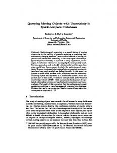
The representation of the objects’ movement is inherently imprecise and therefore, answers to user queries based on such information may be inaccurate [8, 13]. Imprecision may be introduced by the measurement process – it may depend on the accuracy of the GPS, for instance –, or by the sampling approach, as depicted below. Notice that the imprecision refers to the spatial dimension only, as it is commonly assumed that measurement instruments are able to determine precisely the time a position sample is taken. As an example, consider the case of a port authority dealing with a spread of toxic waste in the sea and querying a nautical surveillance system to know which ships have crossed the polluted zone during a specified time interval. Imagine that the ship responsible for the waste has actually followed the trajectory represented in Figure 1. The black dots represent four observations made during the specified time interval, the shaded region represents the polluted area and the hatched line a trajectory that might have been inferred from the observations.
Figure 1: Uncertainty about moving objects trajectories
The hatched line does not cross the shaded region and, thus, an answer to a query based on this estimation of the trajectory would not include the guilty ship. On the contrary an answer may also include false candidates whose inferred trajectory crosses the area even though they have not actually been there.
2.2
Bounding uncertainty
There are physical constraints on the movement of objects allowing limiting uncertainty of their position at a certain time. For instance, the uncertainty zone for a train moving on a railway is a section of the railway and for a ship moving freely in the ocean is an area. When it comes to future movements, considering a two-dimensional space (Figure 2), the uncertainty area is a circle centered on 2.1 Uncertainty of past, present and the expected location of the object. The circle bounds the maximum deviation allowed for future positions an object at a given time instant. Objects are committed to send a location update when the The preceding example focuses on the history deviation reaches the bound. of the objects’ movement. In general, the focus may be put on the past movement or on the future movement of objects, depending on applications requirements. Two main approaches were raised. The first approach [8, 6], focusing on past movements, addresses the needs of mining applications of spatiotemporal data: traffic mining, environment monitoring, etc. In this case, uncertainty is bounded using a sequence of positions of objects and some known physical constraints on their movement. Figure 2: Expected location of a moving object In the second approach [10, 11, 19, 13], the focus is put on the uncertainty about the fuFor past movements, since the positions beture movement of objects. This approach ad- tween two consecutive samples are not meadresses the needs of real-time applications and sured, the best to do is to limit the poslocation-based services: real-time traffic con- sibilities of where the moving object could trol, real-time mobile workforce management, have been [9, 8, 7]. Let us consider a twodigital battlefields, etc. These systems make dimensional space and a moving object m, an use of speed patterns information in the con- instant t belonging to a time interval ht1 , t2 i struction of future movements and uncertainty and two consecutive observations (p1 , t1 ) and is fixed in advance. The latter allows avoid- (p2 , t2 ), (Figure 3). We denote by p1 and p2 ing frequent updates of the database. In fact, the positions of the moving object at observathe database is not updated as long as the ac- tion time instants t1 and t2 , respectively. d detual object’s movement deviation from its ex- notes the distance between p1 and p2 . At time pected location, as inferred from the informa- t, the distance d1 between m and p1 is inferior tion stored in the database, is less than the to r1 = Vmax × ∆t1 , where ∆t1 = t − t1 and threshold previously fixed. Vmax is a user-defined value standing for the
maximum velocity of moving object m. The distance d2 between m and p2 , at instant t, is inferior to r2 = Vmax ×∆t2 , where ∆t2 = t2 −t. So, at time t, the moving object might be at any location within the area defined by the intersection of the two circles of radius r1 and r2 . This is a so-called lens area [8] representing the set of all possible locations for a moving object at a certain time instant.
intersection of the two circles with the ellipsis. Lens areas for time intervals comprising one or more observations are the union of several lens areas computed using the method described above.
2.3
Using probabilistic methods
Consider now that we have methods that allow estimating the location of a moving object at any time instant. The evaluation of spatiotemporal query expressions could than be augmented with probabilistic estimates of the validity of answers to users queries. Thus, it would be possible to answer queries such as Figure 3: A lens area for a time instant “Which are the planes for which the probability of being inside Area C within 5 minutes is The set of all locations where a moving obat least 40%?”, or “Which were the ships that ject might have been between two consecutive were in a certain area during a given time inobservations corresponds to an ellipsis (Figterval, with a probably of at least 60%?”. ure 4). This means that the ellipsis covers all Figure 5 illustrates this kind of query [8]. possible lens areas between the two consecutive It considers the case of the anticipation of observations [7, 2]. the location of an object moving on a twodimensional space. If we assume that the distribution of probability in this lens area is uniform, then, the object is said to be within the given area with a probability of 30%, if at least 30% of its lens area is within that area. Figure 4: A lens area for a time interval between consecutive observations Figure 4 shows how to compute the lens area for a time interval hta , tb i, between two consecutive observations. The circle with radius rb = Vmax × (tb − t1 ) corresponds to the maximum distance from p1 that could be reached by the moving object at tb . The same reasoning applies to ra . In addition, the moving Figure 5: Probability of intersection between a object could not have been outside the ellipsis lens area and a query window just defined. So, the lens area is defined by the
2.4
Related works
In recent years, uncertainty handling emerged as an important issue in moving object database research. Several aspects were investigated and two complementary models were proposed: [8] focusing on past objects’ movement and [19, 13] dealing with future objects’ movement. Moreover, [18, 17] investigated the communication cost for updating the database in the case of real-time applications. [5] discusses how the uncertainty of network constrained moving objects can be reduced by using reasonable modeling methods and location update policies. Finally, [9] added fuzziness in object location and considered the case of moving objects that may change their geometry in time. An important issue of the current research activity in this domain is the design of a probabilistic model of uncertainty. The goal is to handle more realistic (non-uniform) distributions of probability on the location of moving objects, and measure the validity of the answers to user queries. Recent results [4, 3, 12] are going toward this goal, even if they just briefly touch upon the possibility of a nonuniform distribution. Besides, the evaluation of user queries may require handling temporal types such as time instants, time intervals or a combination of them. Evidently, the probability of presence of a moving object within a given area at a certain time, should be less or equal than the probability of presence of the moving object within the same area during any time that includes the previous one. However, the methods presented in section 2.3 are suitable for dealing only with time instants and are not adequate to deal with time intervals. For instance, consider figure 6 where A is an area of interest, L0 is the lens area calculated for the location of an object at a time instant t (1st case) and L00 is a lens area for the loca-
tion of the same object during a time interval hta , tb i ⊃ t (2nd case).
(1st case) Lens area for t
(2nd case) Lens area for hta , tb i ⊃ t
Figure 6: Intersection of a lens area (L) with an area of interest (A) Considering that the distribution of probability in the lens area is uniform, then the probability of presence of the moving object within 0) A at time t is P (t) = area(A∩L area(L0 ) and the probability of being within A during time hta , tb i is 00 ) P (hta , tb i) = area(A∩L area(L00 ) . As A ∩ L0 is equal to A ∩ L00 and the area of L0 is less than the area of L00 then, against evidence, P (t) is greater than P (hta , tb i).
3
Probabilistic reasoning
This section presents the statistical tools that we propose for the evaluation of probabilistic estimates about the location of moving objects. We will denote the probability of presence of a moving object within a given region during a certain time, simply as P (t). We only consider the past objects’ movement and we assume that it is represented as an ordered sequence of observations, denoted {(t, p)}, where p is a two-dimensional value denoting the location of the object at time instant t. We also consider that the objects move freely in space with no obstacles or networks constraining their movements. It is also important to notice that the movement of real-world objects is not random. Indeed, it is reasonable to consider that, most often, their movement is smooth, i.e., that the
movement between two locations is approximately linear and uniform. This means that the locations in the neighborhood of the position expected for an object1 , denoted p˜, should have a greater weight in the computation of the probabilities, than those locations that are far from p˜. As we are interested in obtaining realist estimates, it is desirable that the density functions for distribution of the probabilities within lens areas take this feature into account. Moreover, the location of a moving object at the time instants corresponding to the observations is precisely known, and thus, we must have P (t) = 1 for those time instants or any time interval containing them. Finally, we also assume that there are systems for which it is not reasonable to estimate in advance the maximum velocity of a moving object with an acceptable accuracy. We propose a specific method for those cases. We have investigated two main guidelines for the implementation of the proposed statistical tools, which were designated by pointbased and trajectory-based approaches. We have developed methods based on each of these approaches and we will put in evidence the strengths and weaknesses of each one.
3.1
Point-based approach
As referred in section 2.4, there are several authors suggesting using a density function to estimate the probabilities of presence of a moving object at each point inside the lens area. Then, assuming that t denotes a time instant, the values of P (t) may be calculated using the weight of the intersection of the lens area with the region considered, as shown in formula (1). 1
The position expected for a moving object at a certain time instant is estimated assuming that the movement between consecutive observations is linear and uniform.
P (t) =
WLensArea(t) ∩ Region WLensArea(t)
(1)
The main issue is the definition of a density function over a complex form, such as a lens area. Since we can easily define a density function over a circle, we propose to perform an anamorphosis of the lens area into a circle. The method that we propose consists in four steps: • First, we define a local coordinates system for the lens area, to make the formulation of the lens area equation easier. • Second, we define the anamorphosis of the lens area into a circle of radius 1, to which the chosen density of probability will be associated. • Third, we define how to transform the density of probability over the circle of radius 1 into a density of probability over the lens area. • Finally, we complete the process by the evaluation of P (t). 3.1.1
Lens area equations
The lens area is given by the intersection of two circles. If one circle contains the other, the result of the intersection is the smaller circle. This situation may arise for time instants in the neighborhood of the instants of observations. Otherwise, the result of the intersection is an area similar to the one depicted in figure 7. The lens area in figure 7 delimits the set of all possible locations for a moving object at time instant t, between two consecutive locations: p0 , observed at instant t0 , and p1 , observed at t1 . As presented in section 2, the left centered circle delimits the lens area of the object during the time interval [t0 , t]. The right centered circle delimits the lens area of this object during
Applying the Al-Kashi’s theorem (law of cosines) [1, 16], we obtain the following abscises for p0 and p1 in the local coordinates system: x0 = − d
(
the time interval [t, t1 ]. The radiuses of the circles depend on the maximum velocity (Vmax ) previously estimated:
To make the formulation of the lens area parameters easier, we use a local coordinates system based on the lens area axes (see figure 7). Let us consider d as the distance between p0 and p1 . The origin o of the coordinates system corresponds to the projection of the lens area summits over the x-axis. Formally, o is considered as the center of mass, i.e. the barycenter2 , of points p0 with mass d=(xx11−x0 ) , and p1 with mass d=(xx10−x0 ) , and is defined as: o
n³ ³ = bar
p0
x0 0
´ ,
x1 d
´ ³ ³ ,
p1
x1 0
´ ,
x0 d
´o (3)
2 Consider two points A1 and A2 defined by their cartesian coordinates (x1 , y1 ) and (x2 , y2 ). The mass, also referred to as the weighting coefficients, for each point is m1 and m2 , respectively. The barycenter of ((A1 , m1 ), (A2 , m2 )) is a point d with cartesian coor2 x2 and yg = dinates (xg , yg ) such as: xg = m1mx11 +m +m2 m1 y1 +m2 y2 . m1 +m2
x0 −
(
(2) r1 = Vmax × (t1 − t)
x1 −
fL (y) =
fR (y) =
r0 = Vmax × (t − t0 )
´
(4)
= d + x0
In the general case, the lens area is defined by two arcs located in the half-plans x > 0 and x < 0. Otherwise, it is a circle centered on p0 or p1 . So, we use the following explicit equations to represent the lens area:
Figure 7: Lens area parameters
0 0
+r0 2 −r1 2 2d
d2 −r0 2 +r1 2 2d
x1 =
³
2
x0 + x1 +
p
r1 2 − y 2
p
2
r0 −
p
y2
, in the general case , if x1 −
p
r1 2 − y 2 > 0
r0 2 − y 2
, in the general case
r1 2 − y 2
, if x0 +
p
p
r0 2 − y 2 < 0 (5)
Now, we can easily change from the global coordinates system µ to the¶local one, by a translation of vector
−o.X −o.Y
, that places the ori-
gin at o, followed by a rotation of an angle θ, such as: (
cos θ = sin θ =
3.1.2
p1 .X−p0 .X d p1 .Y −p0 .Y d
(6)
Lens area anamorphosis
As referred above, defining a density function over complex objects such as lens areas would not be a simple task. To cope with this problem, we propose using an anamorphosis, to transform the lens area into a circle of radius 1 (figure 8). The density function will be then defined over the circle. To achieve such transformation, we define an affine bijection [15, 14] between the lens area and the circle. This one-to-one transformation preserves collinearity (i.e., all points lying on
- Let us denote the maximum height of a lens area by r. Depending on the shape of the lens area, r may be equal to the length of the line segment between the summits of the lens area (figure 8(a)), or it may be equal to the radius of the smaller of the two circles that define the lens area. The latter occurs for time instants near to the instants of observations, when the lens area is a circle or when it looks like the one presented in figure 8(b). Equation 8 shows how to calculate r.
(a) 1st case
( p
(b) 2nd case
r0 2 − x0 2
r=
r0 r1
Figure 8: Lens area anamorphosis a line initially still lie on a line after transformation), as well as the ratios of masses and distances (i.e., the barycenter of a line segment stills the barycenter of the corresponding line segment after transformation). So, determining the point in the circle that corresponds to a point in the lens area, is formally defined as follows: - Consider a point
³ M
x y
´
that belongs the
lens area (figure 8). - Using the explicit equations (5), we can define the endpoints of³ the line´ segment containing M , as Ll xL =yfL (y) and ³
Rl
xR = fR (y) y
´
µ Lc
p
−
M = bar
Ll ,
xR − x xR − xL
1−
y2 r
y r
n³
´ ³ , Rl ,
x − xL xR − xL
(7)
and Rc
1−
y2 r
y r
(9)
Lc ,
xR − x xR − xL
´ ³
x − xL xR − xL
, Rl ,
´o (10)
- So, P is the image of M obtained by an anamorphosis α such as:
³
´o
µ p
- Point P in the unity disk is the image of M , obtained by an affine one-to-one transformation of line segment Ll Rl in the lens area into the line segment Lc Rc in the unity disk:
P = bar
n³
(8)
- The points Lc and Rc in the boundary of the unity disk (figure 8), that correspond to the points Ll and Rl in the boundary of the lens area, are defined as follows:
.
- Supposing that M is the barycenter of the line segment Ll Rl , then M must verify equation (7). This means that mass coefficients of Ll and Rl are proportional to their distance from M .
, in the general case , if x0 > 0 , if x1 < 0
M
x y
´
à α
→P
q 2x−xL −xR xR −xL
1− y r
¡ y ¢2 ! r
(11)
3.1.3
3.1.4
Defining the density function
The density of probability over the lens area is then defined throw the density of probability over the unity disk. However, we cannot simply apply the transformation and keep the probability corresponding to each point, since the differential surface element has been changed by the anamorphosis: R L
f (α (x, y)) dx dy 6=
R D
(12)
D stands for the unity disk.
Hence, the density of probability must be normalized to guarantee that the whole probability is equal to 1. As in computation it is not possible to deal with infinite sets, we have introduced the notion of granularity g in this model. We define g as the distance between two consecutive points (granules). So, the coordinates of each point become multiples of g. We define the weight of a point as its corresponding density of probability over the unity disk. Considering all the points in a lens area, the sum of their weights gives the total weight of the lens area Wtot . Wtot = X
X
m>0|m g−x0