Proc. of the 2003 ACM SIGPLAN Conf. on Languages, Compilers and Tools for Embedded Systems, San Diego, CA June 2003
Profiling Tools for Hardware/Software Partitioning of Embedded Applications Dinesh C. Suresh
Walid A. Najjar
Frank Vahid
University of California, Riverside
[email protected]
University of California, Riverside
[email protected]
University of California, Riverside
[email protected]
Jason R. Villarreal
Greg Stitt
University of California, Riverside
[email protected]
University of California, Riverside
[email protected]
ABSTRACT Loops constitute the most executed segments of programs and therefore are the best candidates for hardware software partitioning. We present a set of profiling tools that are specifically dedicated to loop profiling and do support combined function and loop profiling. One tool relies on an instruction set simulator and can therefore be augmented with architecture and microarchitecture features simulation while the other is based on compile-time instrumentation of gcc and therefore has very little slow down compared to the original program We use the results of the profiling to identify the compute core in each benchmark and study the effect of compile-time optimization on the distribution of cores in a program. We also study the potential speedup that can be achieved using a configurable system on a chip, consisting of a CPU embedded on an FPGA, as an example application of these tools in hardware/software partitioning.
Categories and Subject Descriptors C.3 [Performance of Systems]: Measurement techniques, Design studies – profiling techniques, hardware/software partitioning.
General Terms Measurement, Performance, Design, Experimentation.
Keywords Hardware/Software partitioning, loop analysis, compiler optimization.
1. INTRODUCTION Embedded software is the key contributor to embedded system performance and power consumption. Program execution tends to spend most of the time in a small fraction of code, a feature known as the “90-10 rule” – 90% of the execution time comes from 10% of the code. By their very nature, embedded applications tend to follow the 90-10 rule even more so than desktop type of applications. Tools seeking to optimize the performance and/or energy consumption embedded software therefore should focus first on Permission to make digital or hard copies of all or part of this work for personal or classroom use is granted without fee provided that copies are not made or distributed for profit or commercial advantage and that copies bear this notice and the full citation on the first page. To copy otherwise, or republish, to post on servers or to redistribute to lists, requires prior specific permission and/or a fee. LCTES ’03, June 11-13, 2003, San Diego, California, USA. Copyright 2003 ACM 1-58113-647-1/03/0006…$5.00.
finding that critical code. Possible optimizations include aggressive recompilation, customized instruction synthesis, customized memory hierarchy synthesis, and hardware/software partitioning [10,2] all focusing on the critical code regions. Of those critical code regions, about 85% of those regions are inner loops, while the remaining 15% are functions. A partitioning tool should focus first on finding the most critical software loops and understanding the execution statistics of those loops, after which the tool should try partitioning alternatives coupled with loop transformations in the hardware (such as loop unrolling). Our particular interest is in the hardware/software partitioning of programs, but our methods can be applied to the other optimization approaches too. Many profiling tools have been developed. Some tools, like gprof, only provide function-level profiling and do not provide sufficient information at a more detailed level, such as loop information, necessary for partitioning. However, tools that profile at a more detailed level tend to focus on statements or blocks – a user interested in loops must implement additional functionality on top of those profilers. Furthermore, many profiling tools, like ATOM [12] or Spix [11], are specific to a particular microprocessor family. Instruction-level profiling tools can be tuned to provide useful information regarding the percentage of time spent in different loops of a program. Instruction profiling tools can be broadly classified into two categories – compilation based instruction profilers and simulation based instruction profilers. A compilation based profiler instruments the program by adding counters to various basic blocks of the program. During execution the counter values are written to a separate file. Simulation based instruction profiler uses an instruction set simulators they can be further classified into static or dynamic profilers. Simulation based dynamic instruction profilers obtain the instruction profile during the execution of the code on the simulator while in static profiling the execution is written to a trace and the trace is processed to get instruction counts. For very large applications, the trace generated by static profiling can grow to unmanageable proportions. Even though a dynamic profiling method is slow compared to the compiler-based instrumentation, a variety of architectural parameters can be tuned and studied while the program gets profiled on a full system simulator. We have developed a profiling tool that focuses on collecting loop level information for a very large variety of microprocessor platforms. Our profiling tool supports both the instrumentation and the simulation paradigms. We achieved this goal by building on top of two very popular tools – gcc for instrumentation, and Simics [9] for simulation – while keeping the output identical for the two
paradigms, enabling easy switching among the paradigms. Both gcc and Simics, and hence our tool, support dozens of popular microprocessors. We call our toolset as Frequent Loop Analysis Toolset (FLAT).
2. RELATED WORK Profilers like gprof are helpful to the extent of determining the time spent on function calls. However, to make judicious hardware/software partitioning decisions, knowledge of the program at the granularity of loops is imperative. ATOM [11] provides a toolset that lets the user track a program’s behavior by inserting analysis routine at interesting parts of the program. When the program is executed, the analysis routines collect information about various parts of the program and dump the result to a separate file. ATOM provides the following tools for instruction profiling-hiprof, pixie and uprof. The hiprof tool is capable of providing sampled program counters for different program events. Pixie tool provides basic block profile information. Uprof is useful for profiling non-time events and can provide procedure, source line and assembler profiles for a program. The Harvard Atom Like Tool (HALT) [3] provides a flexible way to add routines to program produced by the SUIF compiler. Users indicate interesting parts of the program by labeling them with SUIF annotations. HALT looks for these annotations, and inserts function calls to analysis routines that match the type of the annotation. Using different analysis routines, Halt provides a number of hardware simulators, performs branch stream analysis, and records statistics for profile-driven optimizations. HALT is helpful for obtaining information regarding branch prediction, code layout, instruction scheduling, and register allocation. It has been ported to MIPS and ALPHA processors. Optimally Profiling and Tracing Programs [4] inserts counters in the CFGs in order to record the execution count of the basic blocks and the program. QPT [15] is an instruction-profiling tool based on the algorithms described in [4] and is targeted for the SPARC architecture. It supports two modes of instruction profiling – a quick mode and a slow mode. Slow mode inserts a counter for every basic block while the quick mode relies on inserting counters on an infrequently executed subset of edges in the control flow graph. CPROF [15] processes program traces generated by QPT and annotates source lines and data structures with the appropriate cache miss statistics. ProfileMe [5] samples instructions as they move through an outof-order issue pipeline and reports statistics like cache miss rates. LooAn [1] is a profiling tool that gives loop and function level information. However, since it’s a static profiler, trace files scale up to unmanageable proportions for very large programs. Shade [15] combines instruction set simulation with trace generation capability. It uses a user-specified trace analyzer to control program execution and the extent of trace generation. The analyzer code is generated dynamically and is cached for reuse. ALTO [16] develops whole-program data flow analysis and code optimization techniques for link time program optimization and is targeted to the DEC Alpha architecture. SpixTool [11] is an instruction profiling toolset intended for the SPARC architecture and it consists of the following two tools – Spix and Spixstat. Spix generate basic block execution profile while Spixstat generates
statistics on instruction count, branch behavior, opcode usage, etc. Loop information can be easily deduced from the tool’s output. The Vtune [13] Performance Analyzer collects, analyzes and displays software performance data from the program-level down to a specific function, module or instruction in a developer's source code. Vtune runs on windows and Linux and is targeted for all Intel processors. Idtrace [17] is an instrumentation tool for Intel architecture on Unix platforms. It produces a variety of trace types like profile, memory reference, and full execution traces. Primitive post-processing tools, which read output files, view traces, and compute basic profile data are included in the IDtrace package. Cacheprof [18] is an execution-driven memory simulator for the x86 architecture. It annotates each instruction that reads and writes memory and links a cache simulator into the resulting executable. Upon execution, the data references are trapped and sent to the simulator. Besides producing a procedure-level summary, Cacheprof reports number of memory references and the number of misses for each line of the source code. FLAT is intended to provide loop/function level information for a wide variety of platforms. FLAT_C works for all platforms to which the GNU C Compiler (gcc) has been ported. FLATSIM is capable of producing loop level statistics for a variety of platforms like x86, Strong ARM, MIPS and SPARC.
3. FLAT: FREQUENT LOOP ANALYSIS TOOLS Instruction profiling tools provide information based on which useful hardware/software partitioning decisions can be made. Frequent Loop Analysis Tool set (FLAT) is a profiling tool written in python and it provides the execution time of a given application at the granularity of both loops and functions. Loop profiles can be obtained through two different ways. The first method is to instrument the compiler to output the frequency of a loop and the other method is to use an instruction set simulator to find the execution count of loops. Both methods have their own advantages and disadvantages. The compilation-based approach is a lot faster while the simulation-based approach would prove to be more
S/w Source Gcc profile
Executable
Basic block count
Objdump Disassembled instructions
FLATC
Loop & Function statistics
Figure 1 Tool flow for FLATC
Executable Objdump Disassembled instructions
FLATSIM
Simics
Loop & Function statistics
Figure 2 Tool flow for FLATSIM beneficial in tuning the various architectural aspects of the program. During hardware/software partitioning, frequently executed functions often prove to be the favorite candidates for hardware mapping. However, a frequently executed function could have many infrequently executed loops that contribute towards the total execution time of the function. Since loops perform the bulk of computation, returns for the silicon real estate would be maximized if a frequently executed loop of the program were chosen instead of the frequent function mentioned above. The output provided by FLAT is useful in deciding whether a loop or function needs to be mapped onto hardware. FLAT considers functions as loops that are iterate once for each call. FLAT comprises of two profiling tools FLATC and FLATSIM. Figure 1 shows the tool flow for FLATC. FLATC uses gcc to obtain the basic block counts of a program. The information regarding the loop names and function calls are obtained from the disassembled instructions. Once the loops and function calls are identified, the percentage execution can be determined from the execution percentage of basic blocks. Since FLATC uses gcc, it is portable across a variety of platforms and there are no restrictions on the kind of code that can be profiled using FLATC. If a code can be compiled using gcc, it can be profiled using FLATC. Compile-time instrumentation adds roughly 15% of the instructions to the binary in order to accomplish profiling. Figure 2 shows the toolflow for FLATSIM. FLATSIM uses Virtutech’s Simics instruction set simulator to do the instruction profiling. Simics is a full system simulation platform, capable of simulating high-end target systems with sufficient fidelity and speed to boot and run operating systems and commercial workloads. Simics provides a controlled, deterministic, and fully virtualized environment for a variety of hardware and software engineering tasks. Hence, We decided to instrument the Simics modules to get realistic instruction profile estimates. Simics is not an open source simulator. However, the source code for the add-on modules is included with the distribution. The functionality of the simulator can be extended by modifying the existing modules or by creating custom modules. One such module
that is supplied with the Simics distribution is the id-splitter module. The id-splitter module in Simics handles all cache accesses and redirects them to the instruction or data cache accordingly. FLATSIM relies on getting the instruction profile from a modified version of the id-splitter module. The suggested modification to the id-splitter module is as follows. A tree structure containing all the loop-addresses is introduced into the id-splitter module. During execution, if an instruction belongs to one of the loops, the counter associated with the loop is incremented. Finally information about loops and function calls are written to a file. FLATSIM analyses this file and prints out information regarding the loop execution. Table 1 shows the output of FLAT for Diffie-Hellman (DH) key exchange application from the NetBench [19] benchmark suite. FLAT maintains a DAG like representation for holding data structures for loops and functions. Every loop and function is associated with a name. The loops and functions are named in a hierarchical fashion. For example, the loop name in Table 1 refers to the first loop in the function called NN_AddDigitMult. The first sub-loop of this loop would be named as . The loop name, number of loop iterations, total number of instructions executed in the loop, percentage of the execution time spent in the loop are the fields printed in FLAT’s output. The function statistic consists of the function name, number of times it was called, static size, total number of instructions executed inside the function and percentage of time spent in the function.
4. BENCHMARKS Table 1 FLAT's output for the DH application Loop Name
Frequency
Loop size
Total Inst. (In Million)
% Exec.
1
54563
4178
100.00
3192157
246
598
14.31
3198863
221
548
13.12
1529347
237
237
5.66
260926
602
80
1.92
691293
137
64
1.53
1384533
57
54
1.29
232447
204
39
0.93
333351
256
33
0.79
280283
139
28.00
0.67
Function Name
Frequency
Loop size
Total Inst. (In Million)
% Exec.
5972388
297
1479
35.39
2985562
365
673
16.12
2986826
339
627
15.01
1436259
319
263
6.28
240351
799
151
3.61
240351
1057
126
3.02
1302080
122
79
1.88
650132
263
78
1.85
212257
421
47
1.11
279953
213
40
0.95
Table 2 Percentage execution time of top 10 loops of SPECINT (Threshold = 5%) Loop Benchmarks
1
2
3
4
5
6
7
8
9
10
No. Of Core Loops
Core
ACLC *
type
Bzip2
18
37
46
55
61
67
73
77
82
85
6
Weak
11.15
Crafty
25
33
40
46
52
57
62
67
71
75
7
Weak
8.84
Eon
3
5
7
9
11
13
15
16
17
18
0
Coreless
0.00
Gap
17
26
34
41
47
51
56
60
63
67
5
Weak
9.30
Gzip
29
43
54
65
73
81
86
90
93
96
6
Strong
13.53
MCF
24
47
58
68
76
83
89
94
94
95
7
Strong
12.66
Parser
8
15
21
27
33
38
43
47
50
54
6
Weak
6.38
Twolf
21
28
35
41
45
49
52
55
58
60
4
Weak
10.25
Vortex
14
23
29
35
37
40
42
43
45
46
4
Weak
8.71
Vpr
30
42
52
60
66
72
77
81
85
87
7
Strong
11.00
Average
19
30
38
45
50
55
59
63
66
68
5
Weak
10.03
Table 3 Percentage execution time of top 10 loops in MediaBench (Threshold = 5%) No. Of Core Loops
Loop Benchmarks ADPCM
1
2
3
4
5
6
7
8
9
10
Core
ACLC *
type
100
100
100
100
100
100
100
100
100
100
1
Strong
99.95
G721decode
47
69
87
92
95
96
97
98
98
97
3
Strong
28.95
G721encode
46
68
85
90
93
94
95
96
97
97
3
Strong
28.36
Jpegdecode
41
67
77
86
89
90
90
90
90
90
4
Strong
21.47
Jpegencode
29
42
54
65
75
84
89
92
93
95
6
Strong
14.03
Mpegdecode
76
81
84
87
89
90
92
93
93
94
1
Strong
76.68
Pegwit
40
71
81
85
89
92
94
97
98
98
3
Strong
26.83
Average
52
69
80
86
89
92
93
94
95
95
4
Strong
21.42
* ACLC – Average Core Loop Contribution We analyze an extensive collection of SPECINT [20] integer applications (mcf, bzip2, vpr, vortex, crafy, parser), MediaBench [21] (ADPCM, G721, MPEG, JPEG, Pegwit), cryptographic applications (AES, 3DES, RC4, RC6, idea, blowfish, seal and sha1) and network applications (dh, drr, tl, route and url - all from NetBench [19]). The benchmarks were compiled for the X86 architecture using the GNU C Compiler (gcc version 2.95.3). The execution times of the first 10 loops of different benchmarks are shown in Tables 2, 3 and 4.
5. CORE IDENTIFICATION We define core as the set of all loops whose execution time is higher than a threshold value. If for an application, no loop contributes more than the threshold value, we classify the application as coreless. We refer to the cores with contribution closer to 90% as a strong core and we refer to cores with contribution is closer to 50% as a weak core. Tables 2, 3 and 4 show the loop contributions from the first 10 loops of SPECINT,
MediaBench and NetBench/security applications respectively. We find that the loop contribution decreases successively as we move towards the tenth loop. We identify the cores across different benchmarks in the following manner. For each application, all frequent loops that take up more than 5%( a fixed threshold) of the total execution time are considered as a part of the core. From Tables 3 and 4, it is clear that embedded system applications like MediaBench, NetBench and cryptographic algorithms have a very high percentage of core contribution. Cryptographic applications tend to have much lesser code size as compared to the media or network applications and are hence characterized by the presence of very strong cores. On an average, the cores for cryptographic applications often consist of two loops. The NetBench applications have strong cores and their core size is 3 loops for most of the applications. Media applications from the SPECINT to be less significant than the core contribution have moderately strong cores while most of the SPECINT applications have weak cores. We
Table 4 Percentage execution time of top 10 loops in Security and NetBench applications (Threshold = 5%)
10
No. Of Core Loops
Loop Benchmarks
1
2
3
4
5
6
7
8
9
Core
ACLC *
type
AES
78
93
97
100
100
100
100
100
100
100
2
Strong
46.50
Blowfish
62
87
93
95
95
95
95
95
95
95
3
Strong
31.10
DES
46
90
94
98
98
98
98
98
98
98
2
Strong
45.00
IDEA
48
87
95
95.
95
95
95
95
95
95
3
Strong
31.67
RC4
95
100
100
100
100
100
100
100
100
100
1
Strong
95.00
RC6
87
100
100
100
100
100
100
100
100
100
2
Strong
50.00
Seal
63
98
100
100
100
100
100
100
100
100
2
Strong
48.93
SHA1
75
98
100
100
100
100
100
100
100
100
2
Strong
48.91
CRC
87
99
100
100
100
100
100
100
100
100
2
Strong
49.45
TL
71
82
90
93
95
97
98
98
99
99
3
Strong
29.90
URL
77
95
99
100
100
100
100
100
100
100
2
Strong
47.47
DRR
26
48
65
80
85
87
91
93
95
95
4
Strong
20.09
Average
68
90
95
97
97
98
98
98
99
99
2
Strong
45.35
* ACLC – Average Core Loop Contribution Table 5 Effect of compiler optimization on instruction cycles in MCF benchmark
find that most of the SPECINT applications have weak cores except for eon, which is coreless.
Un-optimized code
For the unoptimized and the optimized versions of each benchmark, Tables 6, 7 and 8 show the total number of instructions in the benchmark, number of instructions in the core of the benchmark and the percentage of instructions contributed by the core. The benchmarks were optimized using the GNU C Compiler (gcc), operating at the highest level of optimization (O3), with loop unrolling enabled.
6. CORE OPTIMIZATION In general, compiler optimization reduces the overall dynamic instruction count of a program. It also involves a lot of code movement and code redistribution. Hence, after optimization, the distribution of cores in a program often gets altered. Table 5 shows the percentage contribution from top four loops of the MCF application in SPECINT suite. One might observe that optimization results in extensive code movement. In Table 5, for the unoptimized version, the second loop in the function has the highest contribution. Due to compiler optimizations such as function inlining, an additional loop is introduced in the function and hence the third loop of the function becomes the most frequent loop after optimization. The contribution of loop increases from 8.28% to 15.91% while that
Optimized code
Loop Name
% Exec
Loop Name
% Exec.
23.44
32.07
18.07
15.91
8.28
13.56
7.54
13.22
Average
74.76
Average
57.33
of loop decreases. Overall, the contribution of the top four loops to the execution time increases from 57% to 75%. Compiler optimizations have a strong impact not only on the size of the computation core but also on its composition and the distribution of the frequently executed loops. If the core is more conducive to optimization than the rest of the program, then most of the optimization would be centered around the core. However, the extent to which the core and rest of the program are affected by optimization largely depends on the
80 60
Loop1
40
Loop2
20
Loop3
0 TL
R L U
sh a1
se al
ro ut e
6 rc
4 rc
na t
ip ch ai ns
id ea
dr r
dh
de s
c cr
bl ow fis
h
Loop4
ae s
%Execution
100
Benchmark
Graph 1 Percentage of execution time spent in the first four loops of Security and NetBench applications
35
% Execution
30 25
loop1
20
loop2
15
loop3
10
loop4
5 0 vpr
perl
gzip
gap
parser
eon
twolf
bzip2
vortex
mcf
crafty
benchmark
100 80 60 40 20 0
loop1 loop2 loop3
benchmark
w it pe g
ec od e m pe gd
m pe ge
nc od e
nc od e jp eg e
ec od e jp eg d
co g7 2
1e n
co 1d e g7 2
ad p
de
de
loop4
cm
% Execution
Graph 2 Percentage of execution time spent in the first four loops of SPECINT
Graph 3 Percentage of execution time spent in the first four loops of MediaBench nature of the application. In order to quantify the impact of optimization on the core, we define a new metric called Core to Program Reduction Ratio (CPRR) – the ratio of decrease in core size to the decrease in program size. CPRR is computed as follows:
CPRR =
Decrease in core instructions Decrease in program instructions
One can visualize any program to consist of core and non-core portions. In the definition of CPRR, the numerator denotes the decrease in core instructions between the unoptimized and optimized programs. The denominator is the decrease in total dynamic instruction count due to optimization. If the decrease in the dynamic instruction count can be considered as being proportional to the extent of optimization, then, a CPRR of 50% would mean that the core and the rest of the program were optimized equally. A CPRR value higher than 50% implies that core is more amenable to optimization as compared to the rest of the program; while a CPRR of less than 50% implies that the impact of optimization on the noncore portion of the program is higher.
As illustrated in the Tables 6,7 and 8, programs like the security and Netbench applications have high CPRR values while applications like the SPECINT benchmarks tend to exhibit lower CPRR. We computed the CPRR for SPECINT in order to show the effect of compiler optimization on the kernels of large applications. Of course, the embedded applications, MediaBench, NetBench and the security applications, consist of small kernels while the SPECINT benchmarks are complete programs. This explains why the computation core in the embedded applications is more explicit and dominant.
7. PARTITIONING FOR CSoC In this section we evaluate the potential speedups that can be achieved by mapping the optimized cores to hardware. Configurable System On Chip platforms (CsoCs) like the Xilinx Virtex II pro [7], Altera Excalibur [8] and the Triscend A7 [6] are examples of a few architectures that prove to be ideal for migrating the core loops to hardware. The obvious objective of migrating code to hardware is the speed-up that can be achieved. One should also note that not all loops are conducive to hardware mapping. Figure 3 shows a target architecture that could benefit by mapping
Table 4 CPRR for Security and NetBench applications Benchmark
AES Blowfish CRC
Program unopt.
Core unopt.
% of core in unopt.
Program optimized
Core optimized
(106 inst.)
(106 inst.)
Program
(106 inst.)
(106 inst.)
% Core in
Decrease in program size
optimized program
CPRR
577
577
99.99
1023
1020
99.75
43.52
99.43
1770
1680
94.94
572
572
100.00
67.70
92.53
56
55
99.81
19
19
100.00
66.79
99.71
DES
4390
4290
97.61
2390
2390
100.00
45.58
94.81
IDEA
2710
2580
95.19
1530
1530
100.00
43.59
88.97
IPChains
26.02
24.09
92.57
11
10
91.63
59.40
93.21
RC4
740
740
99.99
328
328
100.00
55.63
99.99
RC6
802
780
97.20
323
323
99.99
59.72
95.40
Seal
168
168
99.94
61
61
100.00
63.73
99.90
6
5
93.12
2
2
90.85
64.26
94.39
1580
1580
99.50
1430
1420
99.65
9.96
98.09
18
15
80.37
16
13
80.33
10.92
80.68
1072
1042
96
642
641
96.58
49.23
94.76
TL URL DRR Average
Table 5 CPRR for SPECINT Benchmark
Program unopt.
Core unopt.
% of core in unopt.
Program optimized
Core optimized
(109 inst.)
(109 inst.)
Program
(109 inst.)
(109 inst.) 4310
%Core in optimized program
Decrease in program size
CPRR
62.87
36.93
58.21
Gzip
10800
6650
61.5
6860
Vpr
12400
7310
58.96
6120
3310
541.6
50.7
63.62
MCF
5470
3480
63.72
2010
1820
90.74
63.22
48
Crafty
14900
6530
43.82
9460
4430
46.79
36.46
38.64
Parser
24600
6670
27.08
12100
4870
40.13
50.72
14.39
Bzip2
13900
7600
54.48
7300
3650
50.01
47.65
59.4
Twolf
23900
9800
40.99
16100
5710
35.49
32.73
52.29
Average
15153
6863
50.03
8564
4014
54.31
45.49
47.79
Table 6 CPRR for MediaBench Benchmark
ADPCM JpegDecode
Program unopt.
Core unopt.
(106 inst.)
(106 inst.)
% of core in unopt. Program
Program optimized
Core optimized
(106 inst.)
(106 inst.)
% Core in optimized program
Decrease in program size
CPRR
56
56
100
32
32
100
43.27
99.99
1930
1660
85.87
1260
1070
84.50
34.66
88.45
JpegEncode
103
67
64.75
77
61
79.43
26.04
23.04
MpegEncode
1280
1100
86.51
917
752
81.95
28.15
98.17
G721decode
1800
1650
91.61
1010
938
93.24
44.15
89.54
G721encode
1920
1720
89.53
1070
947
88.58
44.33
90.72
Average
1181
1042
86.37
728
633
87.95
36.76
81.65
Table 7 Speedup and cumulative execution percentages for the top five loops of SPECINT Loop Benchmarks
1
2
Speedup
3
4
5
Bzip2
19.55
30.19
45.94
50.86
Crafty
24.23
32.68
40.09
Gzip
31.36
45.89
59.46
MCF
32.47
64.58
83.72
1
2
3
4
5
59.16
0.77
0.83
0.96
1.01
1.10
46.79
52.21
0.79
0.85
0.91
0.97
1.02
67.96
77.46
0.84
0.96
1.10
1.22
1.37
90.7
97.35
0.85
1.17
1.50
1.68
1.89
Parser
14.26
23.50
32.19
40.13
47.35
0.74
0.79
0.85
0.91
0.97
Twolf
24.37
29.74
37.44
42.90
48.68
0.79
0.83
0.89
0.93
0.99
Vortex
14.80
26.63
29.19
37.22
41.14
0.74
0.81
0.83
0.89
0.92
Vpr Average
29.2
32.79
44.62
54.16
61.08
0.83
0.84
0.95
1.04
1.12
23.78
35.75
46.58
53.84
60.55
0.79
0.89
1.00
1.08
1.17
Table 10 Speed up and cumulative execution percentage of top five loops in MediaBench Loop 1
2
Speedup
3
4
5
1
2
3
4
5
Benchmarks ADPCM
99.94
99.99
99.99
99.99
99.99
1.99
1.99
1.99
1.99
1.99
G721decode
46.42
72.15
88.23
93.24
96.31
0.96
1.28
1.64
1.76
1.86
G721encode
38.62
67.24
80.11
88.57
92.73
0.90
1.21
1.43
1.62
1.74
Jpegdecode
50.66
66.31
78.07
84.67
88.15
1.00
1.19
1.39
1.53
1.61
Jpegencode
50.08
60.75
71.35
79.66
86.17
1.00
1.12
1.27
1.42
1.56
Mpegdecode
60.16
68.13
74.34
78.75
82.22
1.11
1.22
1.32
1.40
1.47
Pegwit
45.79
80.22
82.91
85.29
87.03
0.96
1.43
1.49
1.54
1.58
Average
55.96
73.55
82.29
89.17
90.37
1.06
1.30
1.47
1.59
1.67
Table 11 Speed up and cumulative execution percentage of top five loops in Security/NetBench Loop 1
2
Speedup
3
4
5
1
2
3
4
5
Benchmarks AES Blowfish DES
91.88
100.00
100.00
100.00
100.00
1.71
1.99
1.99
1.99
1.99
96.5
99.85
100.00
100.00
100.00
1.86
1.99
1.99
1.99
1.99
61.64
91.41
97.04
99.95
99.99
1.13
1.70
1.88
1.99
1.99
IDEA
64.45
97.09
100.00
100.00
100.00
1.17
1.88
1.99
1.99
1.99
RC4
100.00
100.00
100.00
100.00
100.00
1.99
1.99
1.99
1.99
1.99
RC6
100.00
100.00
100.00
100.00
100.00
1.99
1.99
1.99
1.99
1.99
SEAL
55.32
98.03
99.99
100.00
100.00
1.05
1.92
1.99
1.99
1.99
SHA1
91.43
99.99
100.00
100.00
100.00
1.70
1.99
1.99
1.99
1.99
CRC
99.06
99.62
100.00
100.00
100.00
1.96
1.98
1.99
1.99
1.99
TL
41.50
67.12
85.79
90.85
94.38
0.92
1.20
1.55
1.69
1.79
URL
76.36
94.89
99.20
99.65
99.91
1.35
1.81
1.96
1.98
1.99
DRR
26.08
47.84
64.11
80.33
84.67
0.81
0.98
1.16
1.43
1.53
Average
75.35
91.32
95.51
97.57
98.25
1.47
1.79
1.87
1.92
1.94
speedup expected on the loop by mapping it to hardware. From past results [1] we have computed this speedup to be 19 in number of cycles. However, our experience shows that the clock frequency that can be obtained on an FPGA is about 10 times lower than a CPU frequency. For the remainder of this analysis we will assume that HS = 1.9.
External Memory
The overall speedup is the ratio of the SW_only_time over the CsoC time. From Tables 9, 10 and 11, it is clear that mapping the first 5 frequent loops gives an average speedup of 1.17, 1.67 and 1.94 for the SPECINT, MediaBench and NetBench/Security applications. It should be noted that not all loops are suitable for mapping on hardware.
On-Chip Memory
L1 Cache
Configurable Logic
CPU
CSoC
Fabric
Figure 3 Target architecture for a CSoC
loops to hardware. One might observe that no additional delay is required to fetch the data for the configurable logic fabric. In this section, we describe an analysis of this speed-up based on the results obtained from the profiling tool. Note that in this analysis we will not assume any overlap in computation between the CPU and the FPGA on the CSoC. This is a pessimistic but fair assumption
8. CONCLUSION We propose a loop analysis toolset to support hardware software partitioning. We provide a Simics based loop analyzer to profile an application and to fine-tune the various architectural aspects of the application. We also provide an instrumentation based loop analyzer that profiles an application without any significant slowdown compared to the actual execution. For a wide range of benchmarks, we identify the cores of the program and then study the effect of compiler optimization on the distribution of cores. We find that the cores are optimized more as compared to the rest of the program. On an average, the contribution from the first 2-4 loops of embedded applications is roughly 90% while the first 6 loops in the Spec bench suite contributes to almost 55% of the execution time. We observe that mapping the first five most frequent loops to hardware is beneficial for MediaBench, Network and Cryptographic applications.
SoCP time = CPU time + FPGA times
ACKNOWLEDGEMENT
CPU time = SW_only_ time – SW_loop_time
This work was supported in part by NSF Award ITR 0083080
FPGA time = SW_loop_time/HS
REFERENCES s= =
[1] J. Villarreal, D. Suresh, G. Stitt, F. Vahid and W. Najjar,
SW_Only_time CPUtime + FPGAtime
“Improving Software Performance With Configurable Logic”, Kluwer Journal on Design Automation of Embedded Systems, November 2002, Volume 7 Issue 4, Pages 325 – 329.
SW_Only_time SW_only_time − SW_loop_time +
SW_loop_time HS
1 SW_loop_time 1 1− (1 − ) SW_Only_time HS 1 = 1 − 0.47 * %loop_execution
=
Where SW_only_time is the time from software only execution and the SW_loop_time is the time taken on a CPU by the loop that will be mapped to hardware. HS (hardware speedup) denotes the
[2] K. Kucukcakar,
K, “An ASIP design methodology for Embedded Systems”, International Workshop on Hardware/Software Codesign, pages 17-21, 1999.
[3] C. Young, The Harvard Atom Like Tool Manual (HALT), http://citeseer.nj.nec.com/121315.html
[4] T.Ball and J.R. Larus. “Optimally Profiling and Tracing Porgrams”, ACM Symposium on Principles of Programming Languages, 1992, Pages 59-70.
[5] J.Dean, J.Hicks, C. Waldspurger, W. Weihl and G. Chrysos, “ProfileMe: Hardware support for instruction-level profiling on out-of-order processors”, In proceedings of International Symposium on Microarchitecture, December 1997.
[6] Altera Corporation. , Altera Excalibur,
http://www.altera.com/products/devices/excalibur/excindex.html
[7] Xilinx Inc. Xilinx Virtex II Pro Handbook, http://www.xilinx.com/publications/products/v2pro/handbook
[8] Triscend Corp., Triscend A-7 Chip, http://www.triscend.com/products/a7.htm
[9] Simics Simulator, http://www.simics.net. [10] V. Bala, E. Duesterwald, and S. Banerjia, “Dynamo: A transparent dynamic optimization system”, In Proceedings of the ACM SIGPLAN '00 Conference on Programming Language Design and Implementation, pages 1--12, Vancouver, Canada, June 2000.
[11] B. Cmelik, “SpixTools Introduction and User’s Manual”, Techincal Report SMLI TR-93-6, Sun Microsystems Laboratory, Mountain View, CA, February 1993.
[12] A. Srivastava and A. Eustace, “ATOM: A system for building customized program analysis tools”, In ACM conference on Programming Language Design and Implementation, Pages 196-205, Orlando, FL, June 1994.
[13] Intel’s Vtune, http://www.intel.com/software/products/vtune/ [14] R. F. Cmelik and D. Keppel, “Shade: A Fast Instruction-Set Simulator for Execution Profiling”, Tech. Rep. SMLI 93-12 and UWCSE 93-06-06, Sun Microsystems Laboratories, Incorporated, and the University of Washington, 1993.
[15] WARTS, http://www.cs.wisc.edu/~larus/warts.html [16] R. Muth, S. Debray S. Watterson, "alto: A Link-Time Optimizer for the Compaq Alpha", Technical Report 98-14, Dept. of Computer Science, The University of Arizona Dec. 1998. [17] J.Pierce and T. Mudge. “IDtrace - A tracing tool for i486 simulation”, In Proceedings of the International Workshop on Modeling, Analysis and Simulation of Computer and Telecommunications Systems (MASCOTS), 419-420, 1994. [18] Cacheprof. http://www.cacheprof.org [19] G. Memik, W.H. Smith and W. Hu, “NetBench: A Benchmarking suite for Network processors”,In Proceedings of International Conference on Computer-Aided Design (ICCAD),Pages 39-42, Nov 2001, San Jose, CA. [20] SPECINT 2000, http://www.specbench.org/cpu2000/ [21] C. Lee, M. Potkonjak, W. H. Smith, “MediaBench: A Tool for Evaluating and Synthesizing Multimedia and Communications Systems”, International Symposium on Microarchitecture, MICRO 30, pages 292-303, December1997, Research Triangle Park, NC.