programmable spectral design and the binary

PROGRAMMABLE SPECTRAL DESIGN AND THE BINARY SUPERGRATING

A DISSERTATION SUBMITTED TO THE DEPARTMENT OF ELECTRICAL ENGINEERING AND THE COMMITTEE ON GRADUATE STUDIES OF STANFORD UNIVERSITY IN PARTIAL FULFILLMENT OF THE REQUIREMENTS FOR THE DEGREE OF DOCTOR OF PHILOSOPHY

Daniel Levner June 2006

© Copyright 2006 by Daniel Levner All Rights Reserved

ii

I certify that I have read this dissertation and that, in my opinion, it is fully adequate in scope and quality as a dissertation for the degree of Doctor of Philosophy. _______________________________________ (David A. B. Miller) Principle advisor I certify that I have read this dissertation and that, in my opinion, it is fully adequate in scope and quality as a dissertation for the degree of Doctor of Philosophy. _______________________________________ (J. M. Xu)

Co‐advisor

I certify that I have read this dissertation and that, in my opinion, it is fully adequate in scope and quality as a dissertation for the degree of Doctor of Philosophy. _______________________________________ (Olav Solgaard) Approved for the University Committee on Graduate Studies.

iii

Abstract Spectral operations such as wavelength selection, power level manipulation, and chromatic dispersion control are key to many processes in optical telecommunication, spectroscopy, and sensing. In their simplest forms, these functions can be performed using a number of successful devices such as the Fraunhofer (“diffraction”) grating, Bragg grating, thin‐film filter (TFF), and dispersion‐compensating fiber (DCF). More complicated manipulations, however, often require either problematic cascades of many simple elements, the use of custom technologies that offer little adjustment, or the implementation of fully programmable devices, which allow for the desired spectral function to be synthesized ab initio. Here, I present the Binary Supergrating (BSG), a novel technology that permits the programmable and near‐arbitrary control of optical amplitude and phase using a simple, robust and practical form. This guided‐wave form consists of an aperiodic sequence of binary elements; the sequence, determined through the process of BSG synthesis, encodes an optical program that defines device functionality. The ability to derive optical programs that address broad spectral demands is central to the BSG’s extensive capabilities. In consequence, I present a powerful approach to synthesis that exploits existing knowledge in the design of “analog” gratings. This approach is based on a two‐step process, which first derives an analog diffractive structure using the best available methods and then transforms it into binary form.

v

Accordingly, I discuss the notion of diffractive structure transformation and introduce the principle of key information. I identify such key information and illustrate its application in grating quantizers based on an atypical form of Delta‐Sigma modulation. As a digital approach to spectral engineering, the BSG presents many of the same advantages offered by the digital approach to electronic signal processing (DSP) over its analog predecessors. As such, it has potential importance for many domains of optical manipulation. This is especially the case when the BSG incorporates reprogrammable means of actuation. The reprogrammable form, which stands as a universal wavelength processor, promises unique benefits to dynamic optical systems.

vi

Acknowledgments I would like to thank my advisors, Prof. David Miller from Stanford University and Prof. Jimmy Xu from Brown University, for their incredible guidance and support. In particular, I must thank Prof. Xu for introducing me to this project so many years ago and for ensuring since then that it has always been possible for me to pursue it, despite its many twists and turns. Similarly, I must thank Prof. Miller for his wonderful mentoring and for his flexibility, understanding and assistance in allowing me to pursue my work unconventionally. My thanks go to Prof. Olav Solgaard for providing me with an objective outlook on both practical and theoretical aspects of my work and for the valuable feedback in which it resulted. I am also very grateful for Prof. Claire Tomlin’s guidance and support, which I have been fortunate enough to receive since my first day at Stanford. I must convey the greatest thanks and appreciation to my friend and colleague Dr. Martin Fay, who has been my partner and faithful travel‐mate through the entirety of this journey. Martin has honored me with his always‐sober outlook, his heartfelt advice on both technical and non‐technical matters, and his incredible amount of patience and willingness to help. In addition, I would like to thank my dear friend Dr. Ronojoy Ghosh whose hospitality, generosity, encouragement and friendship have meant a very great deal to me.

vii

I would like to thank the friends and supporters of Digital LightCircuits, and all those who helped Martin and I build it. In particular, I would like to mention Ian Ainsworth, Jeff Weiss, Bill O’Farrell and Fred Bamber for believing in us and in our work. I am very grateful for having been chosen for the Stanford Graduate Fellowship (SGF) – a remarkable program that has permitted me not only to pursue my interests but to do so in an unconventional way. I also gratefully acknowledge support from the Defense Advanced Research Projects Agency (DARPA), National Science Foundation (NSF), and Photonics Research Ontario (PRO). Not least, I thank my parents, Ada and Hertz, for standing behind me – always and unconditionally.

viii

Contents Abstract................................................................................................... v Acknowledgments ................................................................................ vii Chapter 1

Chapter 2

Introduction

1

1.1

Spectral Engineering: Why? .............................................................. 1

1.2

Spectral Engineering: How?.............................................................. 5

1.3

The Binary Supergrating (BSG) ........................................................ 7

1.4

The Reprogrammable BSG ................................................................ 9

1.5

The BSG Advantage ........................................................................... 9

1.6

Manuscript Overview ...................................................................... 11

1.7

Intellectual Property Statement ...................................................... 13

1.8

Bibliography ...................................................................................... 13

Background Concepts 2.1

2.2

2.3

17

Electromagnetic Waves.................................................................... 17 2.1.1

Plane waves and refractive index...................................... 19

2.1.2

Refraction.............................................................................. 20

Optical Waveguides ......................................................................... 22 2.2.1

Guided modes and modal index ....................................... 23

2.2.2

Waveguide dispersion ........................................................ 25

2.2.3

Evanescent tails.................................................................... 26

Transfer Matrix Methods................................................................. 27 2.3.1

S‐matrix formulation........................................................... 28

ix

2.4

2.5

Chapter 3

ABCD‐matrix formulation.................................................. 29

2.3.3

Extended formulations ....................................................... 30

Linear System Analysis and Control ............................................. 31 2.4.1

Rational‐form continuous‐time systems and stability ... 32

2.4.2

Discrete‐time Fourier transform ........................................ 34

2.4.3

Rational‐form discrete‐time systems and stability ......... 35

2.4.4

Spectral resolution ............................................................... 36

2.4.5

Causality ............................................................................... 37

Bibliography ...................................................................................... 38

Past Approaches

41

3.1

Thin‐film filters ................................................................................. 41

3.2

Raman‐Nath Diffraction .................................................................. 42

3.3

Fiber Bragg Gratings ........................................................................ 45

3.4

Analog Gratings in Waveguides .................................................... 47

3.5

Chapter 4

2.3.2

3.4.1

Superimposed photoinscription ........................................ 48

3.4.2

Grayscale lithography......................................................... 48

3.4.3

Electro‐optic gratings in lithium‐niobate ......................... 50

Binary Gratings in Waveguides...................................................... 51 3.5.1

Sampled grating (SG) .......................................................... 51

3.5.2

Superstructure grating (SSG) ............................................. 52

3.5.3

Binary superimposed grating ............................................ 53

3.6

Conclusions ....................................................................................... 54

3.7

Bibliography ...................................................................................... 54

BSG Synthesis & Key Information

57

4.1

The Principle of Key Information................................................... 58

4.2

The Fourier Approximation ............................................................ 59

4.3

Delta‐Sigma Modulation ................................................................. 62

4.4

Second‐Order Considerations......................................................... 66

4.5

The Baseband Exclusion Principle ................................................. 68

4.6

Conclusions ....................................................................................... 70

4.7

Appendix – Key Derivations........................................................... 71 4.7.1

The Fourier approximation ................................................ 71

4.7.2

Second‐order coupling coefficients................................... 72

4.7.3

Baseband exclusion width.................................................. 75

x

4.8

Chapter 5

Analog Grating Synthesis 5.1

Modes of Grating‐Assisted Coupling ............................................ 79 5.1.1

Co‐linear couplers ............................................................... 80

5.1.2

Co‐planar couplers .............................................................. 84

Inverse Scattering Theory................................................................ 86

5.3

Iterative Fourier Methods................................................................ 87

5.4

Impulse Response Methods ............................................................ 90 5.4.1

Causality in counter‐directional gratings......................... 90

5.4.2

Causality in co‐directional gratings .................................. 91

Special Concerns ............................................................................... 95 5.5.1

Infinite impulse response (IIR) gratings........................... 95

5.5.2

Chromatic dispersion.......................................................... 97

5.6

Conclusions ....................................................................................... 98

5.7

Bibliography ...................................................................................... 98

Delta-Sigma Modulation

101

6.1

Threshold Quantization................................................................. 101

6.2

Classical Delta‐Sigma Modulation Theory ................................. 103

6.3

6.4

Chapter 7

79

5.2

5.5

Chapter 6

Bibliography ...................................................................................... 76

6.2.1

Noise‐to‐output transfer function ................................... 103

6.2.2

Oversampling ratio ........................................................... 105

Band‐pass Delta‐Sigma Modulation ............................................ 106 6.3.1

Loop stability...................................................................... 107

6.3.2

Filter design ........................................................................ 107

6.3.3

Multi‐band modulators .................................................... 109

6.3.4

Input scaling....................................................................... 110

6.3.5

Multi‐level quantization ................................................... 111

Future Directions ............................................................................ 111 6.4.1

Sub‐bit modulation............................................................ 111

6.4.2

DSM‐based direct synthesis ............................................. 112

6.5

Conclusions ..................................................................................... 113

6.6

Bibliography .................................................................................... 113

Direct BSG Synthesis 7.1

115

Transfer Matrix Optimization....................................................... 116

xi

7.2

Chapter 8

Choice of start structure.................................................... 118

7.1.2

Cost function ...................................................................... 118

7.1.3

Inequality constraints........................................................ 119

7.1.4

Performance........................................................................ 121

Simulated Annealing...................................................................... 122 7.2.1

Principle of operation........................................................ 124

7.2.2

Fast annealing .................................................................... 125

7.2.3

Multi‐agent methods......................................................... 126

7.2.4

Performance........................................................................ 127

7.3

Direct vs. Two‐Step Synthesis: Comparison............................... 128

7.4

Bibliography .................................................................................... 129

BSG Implementation 8.1

8.2

8.3

Chapter 9

7.1.1

131

BSG Design Rules ........................................................................... 131 8.1.1

Spectral Resolution............................................................ 131

8.1.2

Bit length............................................................................. 134

Grating Morphologies.................................................................... 135 8.2.1

Etched or deposited cladding .......................................... 135

8.2.2

Lateral satellite gratings.................................................... 136

8.2.3

Waveguide width variation ............................................. 137

Design of Counter‐Directional Couplers..................................... 137 8.3.1

Asymmetric couplers ........................................................ 138

8.3.2

Symmetric couplers........................................................... 140

8.4

Design of Co‐Directional Couplers .............................................. 141

8.5

A Note regarding Supermodes..................................................... 144

8.6

Conclusions ..................................................................................... 146

8.7

Bibliography .................................................................................... 146

Reprogrammable BSGs

147

9.1

Reprogrammability: Why? ............................................................ 147

9.2

Reprogrammability: How?............................................................ 148

9.3

Thermal Actuation.......................................................................... 150 9.3.1

9.4

Micro‐Electromechanical (MEMS) Actuation............................. 152 9.4.1

9.5

Differential heating............................................................ 151 Index matching fluid......................................................... 153

Liquid‐Crystal (LC) Actuation...................................................... 153

xii

9.6

Chapter 10

9.5.1

Surface alignment layer .................................................... 155

9.5.2

Flip‐chip bonding .............................................................. 157

Hitless Switching ............................................................................ 158 9.6.1

Intrinsically hitless operation........................................... 160

9.6.2

Programmatically hitless operation ................................ 161

9.7

Conclusions ..................................................................................... 162

9.8

Bibliography .................................................................................... 163

Experimental Progress

165

10.1 Counter‐Directional Couplers ...................................................... 165 10.2 Co‐Directional Couplers ................................................................ 171 10.3 Liquid‐Crystal Reprogrammable BSGs ....................................... 176 10.3.1 Bulk LC actuation of waveguide devices....................... 176 10.3.2 LC alignment on waveguide using LPP......................... 178 10.3.3 Fixed‐program BSG in LC ................................................ 179 10.3.4 CMOS‐controlled BSG in LC............................................ 181 10.4 Other Work...................................................................................... 183 10.4.1 Self‐collimated multi‐wavelength lasers ........................ 183 10.4.2 Tunable distributed feedback (DFB) lasers.................... 184 10.5 Conclusions ..................................................................................... 184 10.6 Bibliography .................................................................................... 184

Chapter 11

Future Directions

185

11.1 Demonstration of a Reprogrammable BSG................................. 185 11.2 Sub‐bit Delta‐Sigma Modulation.................................................. 186 11.3 Analog Synthesis under Chromatic Dispersion ......................... 186 11.4 Improved Optimization‐based Synthesis.................................... 187 11.5 Sectionally Tuned BSG................................................................... 188 11.6 Two‐Dimensional BSG Synthesis ................................................. 188 11.7 Conclusions ..................................................................................... 189

Chapter 12

Conclusions

191

xiii

List of Tables Table 2.1:

The basic constants of electromagnetism [3]. ................................................................. 20

Table 7.1:

A comparison between optimization‐based direct BSG synthesis and the two‐ step approach of Chapter 4. ............................................................................................ 128

Table 10.1:

Dimensions and modal parameters for the reflective lateral‐satellite BSG devices in silicon‐on‐insulator (SOI), as indicated in Figure 10.2a............................ 167

Table 10.2:

Dimensions and modal parameters for the cross‐guide counter‐directional lateral‐satellite BSG couplers implemented in silicon‐on‐insulator (SOI). Measurements are indicated in Figure 10.2b................................................................ 168

Table 10.3:

Sample dimensions and modal parameters for the co‐directional BSG couplers implemented in silicon‐nitride (SiN). Measurements are indicated in Figure 10.7. 172

Table 10.4:

Approximate dimensions for the LC‐actuated Mach‐Zehnder interferometer illustrated in Figure 10.12 and produced in silicon‐on‐insulator. ............................. 177

xiv

List of Figures Figure 1.1:

A point‐to‐point optical data link employing wavelength division multiplexing (WDM). Multiple wavelengths are multiplexed onto a single fiber at the source and demultiplexed at the destination. ...............................................................................2

Figure 1.2:

Multi‐node WDM network. Individual network nodes are implemented using a) complete optical demultiplexing and electronic add/drop multiplexing followed by retransmission; or b) optical add/drop multiplexing (OADM), which allows all‐optical pass‐by and avoids retransmission..........................................3

Figure 1.3:

Characteristic drop‐channel spectrum for a three‐band optical add/drop multiplexer (OADM). Marked are the through‐channel isolation and the desirable flat tops of the stop‐bands...................................................................................4

Figure 1.4:

A comparison of the Raman‐Nath (“free‐space”) and Bragg regimes. a) In the Raman‐Nath regime: a diffractive micro‐electromechanical system (MEMS) with ribbon‐like reflective actuators illuminated by lens‐spread light [9]. b) In the Bragg regime: a fiber Bragg grating, which operates within an optical fiber and reflects a selected wavelength band back into its input...........................................6

Figure 1.5:

A form of the Binary Supergrating (BSG) employing an etched partial top cladding to attain aperiodic modulation of the waveguide’s effective refractive index. Proper choice of the binary modulation pattern can produce near‐ arbitrary spectral features; the process of determining this pattern is known as BSG synthesis. .......................................................................................................................7

Figure 1.6:

Binary modulation’s immunity to nonlinearity: any error in the modulation levels still leaves them lying on a straight line. This corresponds to an affine (linear) transformation and does not induce nonlinear distortion of the spectrum.................................................................................................................................8

xv

Figure 1.7:

Three different simulated spectra belonging to BSG devices that differ only in their programs. These correspond to a) optical add/drop multiplexing, b) dispersion‐slope compensation, and c) channel power equalization. ........................ 10

Figure 1.8:

Graceful degradation of a short 300‐bit BSG in the face of individual bit flips. The response is milder the more bits there are in the BSG. .......................................... 10

Figure 2.1:

Reflection and transmission at a normal refractive‐index interface............................ 21

Figure 2.2:

Refraction at an off‐normal refractive‐index interface. ................................................. 22

Figure 2.3:

Guided‐wave propagation viewed as light trapped in the core region by total internal reflection (TIR). For TIR to occur, the core and cladding must be selected such that nclad n2 and θ1 is sufficiently large, the right‐hand‐side of (2.15) can be greater than 1, making it impossible for the equation to be satisfied for any real θ2. This situation is known as total internal reflection (TIR) and implies that no light is transmitted – the index interface acts as a perfect mirror. The angle θ1 at which TIR first occurs is called the critical angle.

2.2

Optical Waveguides

Optical waveguides are devices that confine light and can be used to direct it much like wiring. They come in two main varieties: one‐dimensional or wire‐like waveguides, which constrain light in two dimensions; and two‐dimensional or slab waveguides, which restrict it to a plane. They are typically made of transparent materials and confine light to a core region by surrounding it with a lower refractive‐index cladding. If light is launched into the guide at a sufficiently oblique angle, total internal reflection can keep it bouncing within (see Figure 2.3). Optical fibers, which are long strands of glass designed to have a higher index center, are a common type of optical waveguide. They are prevalent because they can carry signals over large distances with little attenuation or impairment. Another variety of waveguides are those manufactured on the surface of a glass or semiconductor

2.2 Optical Waveguides

23

substrate. These form the basis of planar lightwave circuits (PLCs), which are microchip‐ like optical devices. Chapter 8 describes several material systems suitable for such waveguides.

nclad Total internal reflection Input

ncore Total internal reflection

nclad Figure 2.3: Guided‐wave propagation viewed as light trapped in the core region by total internal reflection (TIR). For TIR to occur, the core and cladding must be selected such that nclad 0), whereas mode 2 remains free to either co‐ or counter‐ propagate. The two modes are assumed to be orthogonal and have modal profiles that are normalized to carry unit power. We suppose further that the system is subject to a spatially varying material profile characterized by the electric permittivity map

60

CHA PTER 4. BSG SYNTHESIS & KEY INFORMATION

ε ( x , y , z ) = ε 0 [ε base ( x , y ) + η Δ ε ( x , y , z ) ] .

(4.2)

Here, ε0 is the permittivity of free space, εbase is the relative permittivity of the z‐invariant material profile to which modes 1 and 2 correspond, and η.Δε is a perturbation to this profile representing the diffractive structure under consideration. η is a “smallness parameter” that scales the perturbation, and Δε is assumed to be non‐zero only in the domain 0 ≤ z ≤ L for some device length L. Coupled mode theory provides the following governing equations for this system [7]:

da 1 = iκ 11 (z )a 1 (z ) + iκ 12 ( z )a 2 ( z )e i (k 2 − k1 ) z dz da 2 i ( k1 − k 2 ) z = iκ 21 ( z )a 1 ( z )e + iκ 22 (z )a 2 ( z ) . dz

(4.3)

Correspondingly, κ11(z) and κ22(z) represent self‐coupling functions imposed by the perturbation, whereas κ12(z) and κ21(z) represent cross‐mode coupling functions. A simple expression for these functions that applies exactly if the two modes are TE‐ polarized and approximately in most other cases is

κ μυ =

ωε 0 4

∫∫ E μ (x , y ) ⋅η Δ ε ( x , y , z ) Eν (x , y ) dxdy . *

(4.4)

x, y

The exact details of the coupling functions beyond their proportionality to η do not affect this derivation, so we abstract the mode‐to‐perturbation overlap integrals in the functions cμν:

κ μυ ( z , ω ) ≡ ηω c μυ ( z , ω ) .

(4.5)

We proceed with a perturbative solution to the coupled differential equations in (4.3) by expanding the modal amplitude coefficient as a power series in the smallness parameter η:

a μ (z ) = η 0 a μ

(0)

(z ) + η 1 a μ (1) (z ) + η 2 a μ ( 2 ) (z ) +

.

(4.6)

4.2 The Fourier Appro ximation

61

Assuming without loss of generality that mode 1 serves as the device input and substituting (4.5) and (4.6) into (4.3), we collect terms in η1. If the two modes are co‐ propagating, this provides the device’s first‐order cross‐port transmission coefficient t21(1) (see Section 4.7.1 for derivation details):

t 21

(1)

≡

η a 2 (1) ( L ) a1

( in )

~ Κ μν ( k ) =

~ = iΚ 21 ( k 2 − k 1 )

∞

∫ κ μν (z )e

− ikz

dz .

(4.7a)

(4.7b)

−∞

Equation (4.7b) can be identified as the Fourier transform of the coupling functions κμν. If instead the modes are counter‐propagating, the analysis yields the first‐order cross‐ port reflectance coefficient r21(1):

r21

(1 )

≡

η a 2 (1) ( 0 ) a1

( in )

~ = − iΚ 21 ( k 2 − k 1 ) .

(4.8)

Both first‐order coefficients are therefore proportional to the coupling function’s Fourier component at k2 – k1, and stand in support of the Fourier approximation. Moreover, expressions (4.7a) and (4.8) identify specific key information: if the structure is to operate over the band of optical frequencies spanning ω1 to ω2, its key information includes the Fourier components of κ21 that lie in a corresponding band of spatial frequencies. This “band of interest” can be defined as

{Κ~ } = {k , Κ~ 21 1

21

(k ) k = ± [k 2 (ω ) − k 1 (ω )], ω 1 ≤ ω ≤ ω 2 }.

(4.9)

Knowledge of this key information enables the development of transformations that modify form but maintain functionality. In particular, it directs the design of quantizers that translate analog structures into binary form through processes that conserve the ~ Fourier information in the { Κ }1 band of interest. BSG synthesis through one such 21

process is presented in the following section.

62


4.3

Delta-Sigma Modulation

To facilitate the pursuing discussion, we adopt the simplifying assumption that the mode‐to‐perturbation overlap integrals cμν defined in (4.5) are independent of optical frequency ω. Although such strict independence rarely exists, it nonetheless serves as a good approximation often even in the presence of moderate dispersion. This assumption allows us to characterize and transform diffractive structures on the basis of their overlap integrals alone, which accordingly become more manageable as one‐ dimensional functions of space, cμν(z). Furthermore, it allows binary structures, which consist of only two types of structural elements, to be described fully by two simple sets of values: cμνh for “high bits” and cμνl for “low bits”. The simplest technique for binarizing diffractive structures is known as “threshold quantization” [8]. According to this method, the analog structure’s mode‐to‐ perturbation overlap integral c21(zi) is compared at equally spaced samples, zi, to a threshold value lying between the binary structure’s overlap integral values c21h and c21l. Each analog sample is thus converted to the “nearest” binary element, regardless of values at other sample points. This technique is very similar to its digital signal processing namesake, and unfortunately shares with it the problem of quantization noise. This “noise” is an expression of the information loss intrinsic to quantization and manifests itself in unwanted spectral features and an often severe deterioration in optical figures of merit. An alternative approach is to keep track of the quantization noise introduced as each sample is binarized and attempt to compensate for it in subsequent samples. This is the basis of Delta‐Sigma modulation (DSM; also referred to as Sigma‐Delta modulation), a quantization technique used in the field of analog‐to‐digital signal conversion that employs such feedback. The canonical DSM is illustrated in Figure 4.2.

4.3 Delta‐Sigma Modulation

63

Figure 4.2: The canonical Delta‐Sigma modulator (DSM) and its noise‐shaping characteristics. Discrete spatial frequency has been normalized to the Nyquist frequency, corresponding to half the sampling rate.

Figure 4.2 additionally illustrates the modulator’s noise‐to‐output transfer function, which is a measure of the quantizer’s “noise shaping” characteristics derived by abstracting the threshold operation as a simple addition of noise [9]. It is important to note that a given quantization technique can only shape the quantization noise spectrum and not avoid it altogether, as information loss is inherent to the quantization process. Consequently, the art of quantizer design lies in choosing the information that survives the process and the fidelity of its reproduction. The canonical DSM forces quantization noise to higher frequencies and preserves Fourier information in the signal’s low‐frequency range (the baseband). Our identified band of key information, however, lies away from the baseband. The canonical DSM can nevertheless overcome this through oversampling: the introduction of multiple binary samples for each analog sample in a proportion known as the oversampling ratio. This expands the quantizer’s discrete frequency scale, which is inversely related to the binary sample length, and extends the baseband to encompass the formerly high‐frequency band of interest. The oversampling ratio further stands as a measure of the attainable fidelity in the conserved band, as the added binary bits increase the signal’s information capacity. Unfortunately, this approach is rarely desirable since oversampling often

64


brings a commensurate increase in the lithographic resolution required to implement the device. A preferred course lies in recognizing that the band of interest constitutes only a fraction of the total (discrete) Fourier spectrum and that this fraction itself stands as a sort of oversampling ratio. This observation motivates the application of an atypical form of DSM known as band‐pass DSM – modulation designed to conserve Fourier information in a specific frequency band. Such modulators are constructed by replacing the canonical DSM’s summation block (“Sigma”) with suitable linear filters that provide the desired noise shaping while maintaining the feedback loop’s stability. The design process can involve a variety of control‐theoretic techniques [10], [11]; it is discussed in detail in Chapter 6. A sample DSM devised for conserving information in the neighborhood of the Nyquist frequency (half the sampling rate) is shown in Figure 4.3. In many applications, the small fraction of the optical spectrum represented by the band of interest represents a sufficient oversampling ratio, allowing for binarization without increase in resolution requirements.

Figure 4.3: An implementation of band‐pass DSM together with suitable filter coefficients.

The DSM approach well suited to BSG synthesis as it quantizes while maintaining specified spatial‐frequency content. Furthermore, DSM algorithms are highly efficient

4.3 Delta‐Sigma Modulation

65

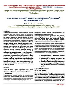
and typically require only linear O(L) computation time with device length L. It is important to note, however, that whereas quantization noise produced outside the band of interest is of secondary importance within the two‐mode model, it may nevertheless contribute to unmodeled effects such as radiation‐mode scattering. Fortunately, these effects can often be minimized through the optimization of mode‐to‐radiation overlap integrals, for example, but still should not be ignored. Figure 4.4 displays the reflectance spectra of two analog implementations of a complex dense wavelength division multiplexed (DWDM) telecom filter, together with the spectra of the BSGs to which they were transformed using the DSM in Figure 4.3. The two analog structures are reflectivity‐scaled versions of the same design, and feature 50GHz channel spacing, ‐40dB stop‐bands, and 25GHz‐wide pass‐bands that are flat to within 0.2dB. The BSG corresponding to the less reflective structure maintains these figures of merit, whereas that corresponding to the more reflective structure deviates noticeably. This degradation in quality with increasing diffractive strength hints that additional key information exists, an issue pursued in the following section.

Figure 4.4: Reflectance spectra corresponding to two analog diffractive structures and the BSGs to which they were transformed using the DSM in Figure 4.3. The analog design in (a) attains a peak‐reflectivity of 1%, whereas that in (b) features a peak‐reflectivity of 81%. The spectra were obtained using the transfer matrix method.

66


4.4

Second-Order Considerations

The foregoing results suggest that the first‐order perturbation analysis that yielded the Fourier approximation is insufficient for strong gratings. Fortunately, the analysis can be extended to uncover the missing key information by considering the model’s second‐ order behavior. To do so, we again substitute (4.5) and (4.6) again into (4.3), but now collect terms in η2. After considerable simplification (see Section 4.7.2), we find the second‐order cross‐port transmission coefficient t21(2) for co‐propagating systems to be

t 21

(2)

≡ t 21 = t 21

(1)

(1)

+

η 2 a 2 (2) ( L) a1

(0)

(0)

i ~ ~ ~ ∫ k [Κ (k ) − Κ (0 )]Κ (Δ k − k )dk

∞

+

22

−∞

3

22

21

3

3

(4.10)

3

i ~ ~ ~ ∫ k [Κ (Δ k − k ) − Κ (Δ k )]Κ (k )dk

∞

−

21

−∞

3

21

11

3

3

.

3

Similarly, the second‐order cross‐port reflectance coefficient r21(2) for counter‐ propagating systems becomes

r21

( 2)

≡ r21

(1)

+

η 2 a 2 ( 2 ) (0) a1

(0)

(0)

= − t 21

(2)

~ ~ − Κ 21 ( k 2 − k 1 ) Κ 22 ( 0 ) .

(4.11)

The integrals in (4.10) and implicitly in (4.11) can be interpreted as follows: for a given optical wavelength, the spatial frequency associated with first‐order coupling corresponds graphically to a vector connecting a start state at k1 to an end state at k2. That is, it is the structure’s Fourier component at k2 – k1 that is relevant. In turn, the integrals resulting from second‐order analysis correspond to two‐step coupling that connects the same endpoints through intermediate “virtual states”. The resulting depictions of Figure 4.5 can be recognized as a form of Feynman diagrams. In this light, the second‐order process comprises two constituents, one corresponding to a cross‐ mode coupling effected by κ21 followed by a same‐mode coupling effected by κ22, the

4.4 Second‐Order Considerations

67

other to a same‐mode coupling effected by κ11 followed by a cross‐mode coupling effected by κ21.

Figure 4.5: Feynman diagrams corresponding (a) to the Fourier approximation and (b) to second‐order analysis.

On first account, it seems that, unlike the first set of key information, the missing second set of key information does not correspond to a specific Fourier band: the second‐order coupling integrals in (4.10) traverse all possible virtual states, thus drawing information from the entire Fourier spectrum. However, closer examination reveals that not all intermediate states participate equally, as transitions with large k3 are highly penalized by the denominator. This resonance is a consequence of the improved phase‐matching experienced by virtual states that neighbor true modes. Accordingly, the practically relevant second‐order transitions combine “low” spatial‐frequency vectors contributed by κ11 and κ22 with “high” spatial‐frequency components contributed by κ21. Beyond a slight widening of the frequency band, the latter components have already been identified as key information in (4.9). The prior components, however, are new. We can therefore summarize the extended collection of key information as

{Κ~ } = {k , Κ~ (k ) k ± Δk (ω ) ≤ δ , ω ≤ ω ≤ ω } {Κ~ } = {k , Κ~ (k ) k ≤ δ } ~ ~ {Κ } = {k , Κ (k ) k ≤ δ } 21 2

21

1

11 2

11

22 2

22

2

(4.12)

Δ k (ω ) = k 2 (ω ) − k 1 (ω ) .

Here, δ represents a limit defining the “low” spatial frequencies that is determined in practice by the desired fidelity in the transformation‐conserved spectral features.

68


4.5

The Baseband Exclusion Principle

The extended set of key information can be incorporated into the DSM approach to BSG synthesis through the use of the so‐called baseband exclusion principle. This principle can be illustrated by reverting to the formalism of wavelength‐independent mode‐to‐ perturbation overlap integrals cμν. As before, each of the binary structure’s bits corresponds to a specific set of these coefficients, allowing us to relate the binary overlap integral functions through linear relations:

c11 ( z i ) =

c 22 ( z i ) =

[

]

c11h − c11l l c 21 ( z i ) − c 21 + c11l h l c 21 − c 21 c c

h 22 h 21

−c −c

l 22 l 21

[c

21

(z i ) − c 21l ] + c 22l

(4.13)

.

Consequently, the spatial frequency information in a binary structure’s c11 and c22 is determined by its c21 content. This observation may seem problematic since it further implies that the binary c11 and c22 are mutually dependent, whereas the corresponding parameters of the analog structure may vary independently. However, it is rarely a pitfall in practice: many analog structures carry no information in the low‐frequency bands identified in (4.12), or else they can be made not to do so. Most others exhibit nearly proportional low‐frequency c11 and c22 content, which can be sufficiently reproduced by a BSG with suitable bit structures. This motivates the definition of a single function, c 21equiv . (z), which carries all the required information: equiv . (z ) = c 21

∞

1 ~ C 21equiv . (k )e ikz dz ∫ 2π − ∞ ~ ~ C 21 (k ) k ∈ K 21

⎧ ~ equiv . ⎪ h l C 21 (k ) = ⎨ c 21 − c 21 ~ l l ⎪ c h − c l C 11 (k ) − c11 + c 21 11 ⎩ 11

[

]

{ } ~ k ∈ {K }

(4.14)

2

11 2

.

Compounding the key information into a single function facilitates improved quantization using the band‐pass DSM infrastructure of section 4.3 with one

4.5 The Baseband Exclusion Principle

69

modification: the addition of a second noise‐free region covering a portion of the spectral baseband. Such augmented modulators maintain both critical bands as c 21equiv . is quantized and are said to employ baseband exclusion. Delta‐Sigma modulators with two noise‐free regions can be designed using many of the same techniques involved in designing single‐band modulators; a sample two‐band modulator is illustrated in Figure 4.6.

Figure 4.6: Band‐pass Delta‐Sigma modulator utilizing baseband exclusion designed to conserve the same spectral features as the modulator in Figure 4.3.

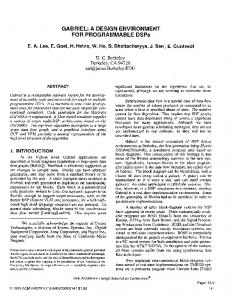
Baseband exclusion modulators must support a sufficiently wide low‐frequency region in order to produce suitable fidelity in the transformed grating’s spectrum. The minimum width this requires varies with application and may be gauged analytically or through iteration (see Section 4.7.3). However, this minimum is often small and can be overestimated with insignificant harm to the oversampling ratio. Exclusions encompassing 1% of the discrete‐frequency scale are typically ample in practice. Figure 4.7 displays the reflectance spectra for the same analog structures as in Figure 4.4, together with the spectra of the BSGs to which they were transformed, this time using the DSM in Figure 4.6. Both BSG structures now faithfully reproduce the desired performance measures and illustrate that modulators employing the baseband exclusion principle indeed overcome the diffractive strength limits that they were conceived to avoid.

70


Figure 4.7: Reflectance spectra corresponding to the same analog diffractive structures as in Figure 4.4 and the BSGs to which they were transformed using the DSM in Figure 4.6, which employs the baseband exclusion principle. The spectra were again obtained using the transfer matrix method.

4.6

Conclusions

The two‐step approach to BSG synthesis affords unprecedented flexibility in the design of Bragg‐domain diffractive spectra by providing a means to harness the knowledgebase of analog grating design. Band‐pass DSM proves well‐matched to the demands of the binarization step of this method and offers structural transformation based on the principle of key information with no attendant increase in lithographic resolution. Through baseband exclusion, band‐pass modulators are capable of quantizing optical structures with strong diffractive features and provide a powerful and efficient method for synthesizing Binary Supergratings. Such gratings enable near‐arbitrary control of spectral amplitude and phase characteristics through a robust and practical form, and stand as a powerful tool for spectral engineering. The principle of key information moreover represents a general approach to diffractive structure transformation and can likewise be employed in the design of other binary and non‐binary Bragg‐regime devices.

4.7 Appendix – Key Derivations

4.7 4.7.1

71

Appendix – Key Derivations The Fourier approximation

Substituting (4.5) and (4.6) into (4.3) and collecting terms in η0 yields the perturbation‐ free behavior, which indicates the absence of modal coupling in the device: (0)

(0)

da 1 dz

a1

(0)

( z ) = a1

(0)

(z) = a2

a2

=

(0)

da 2 dz

= 0 .

( 0 ) = a1

(0)

(0)

(0) = a 2

( L ) ≡ a1

(0)

(4.15a)

( in )

(L) ≡ a2

( in )

.

(4.15b)

As the system is linear, we can simplify the derivation without loss of generality by assuming that mode 1 serves as the device input and setting a2(in) = 0. Collecting terms in

η1 corresponds to a first‐order perturbation: (1 )

da 1 ( in ) = i ω c 11 ( z )a 1 dz (1 ) da 2 ( in ) − iΔ kz = i ω c 21 ( z )a 1 e . dz

(4.16)

Correspondingly, we define Δk = k2 – k1. Equation (4.16) can be integrated directly:

a1 ( z ) = i ω a1 (1)

( in )

z

∫ c (z ′)dz ′ 11

(4.17a)

0

a2

(1)

(z) = a2

(1)

( 0 ) + iω a 1

( in )

z

∫ c (z ′) exp (− iΔ kz ′)dz ′ . 21

(4.17b)

0

Finding the system’s end‐to‐end functionality requires evaluating (4.17b) at z = L. Fortunately, the perturbation’s restriction to 0 ≤ z ≤ L permits a simple result:

72


a2

(1)

( L) = a 2

(1 )

( 0 ) + iω a 1

( in )

L

∫ c (z ′) exp (− iΔ kz ′)dz ′ 21

0

= a2

(1 )

( 0 ) + iω a 1 ∞

~ C 21 ( k ) =

( in )

(4.18a)

~ C 21 ( k 2 − k 1 )

∫ c (z )e

− ikz

21

dz .

(4.18b)

−∞

~ C 21(k) can be recognized as the spatial Fourier transform of c21(z).

When the two‐mode system is co‐propagating (i.e. Re(k2) > 0) we can set a2(1)(0) = 0 in (4.17a) and write the device’s first‐order cross‐port transmission coefficient t21(1) as

t 21

(1)

≡

η a 2 (1) ( L ) a1

( in )

~ Κ μν ( k ) =

∞

~ = iΚ 21 ( k 2 − k 1 )

∫ κ μν (z )e

− ikz

dz .

(4.7a)

(4.7b)

−∞

If instead the modes are counter‐propagating, we can set a2(1)(L) = 0 in (4.17a) and solve for the first‐order cross‐port reflectance coefficient r21(1):

r21

4.7.2

(1)

≡

η a 2 (1) ( 0 ) a1

(0)

(0)

~ = − iΚ 21 ( k 2 − k 1 ) .

(4.8)

Second-order coupling coefficients

We substitute (4.5) and (4.6) again into (4.3) and now collect terms in η2: (2)

da 1 (1) (1 ) = i ω c11 ( z )a 1 + iω c 12 ( z )a 2 e iΔ kz dz (2) da 2 (1) (1 ) = i ω c 22 ( z )a 2 + iω c 21 ( z )a 1 e − iΔ kz . dz

(4.19)

Assigning a1(1) and a2(1) in (4.19) to their expressions from (4.17a) and (4.17b) respectively, integrating to z = L, and employing the limited domain of the perturbation (0 ≤ z ≤ L) yields


a2

(2)

(L) = a2

(2)

73 L

( 0 ) + iω a 2 ( 0 ) ∫ c 22 ( z ′ )d z ′ (1)

0

− ω 2 a1

∞ z ′′

∫ ∫ c (z ′′)c (z ′)exp (− iΔ kz ′)d z ′d z ′′

( in )

22

21

(4.20)

−∞ 0

− ω 2 a1

∞ z ′′

( in )

∫ ∫ c (z ′′)c (z ′ )exp (− iΔ kz ′′)d z ′d z ′′ . 21

11

−∞ 0

Equation (4.20) can be brought into the Fourier domain using the inverse Fourier relations

c μν

1 2π

(z ′ ) exp (− iΔ kz ′ ) =

1 2π

c μν ( z ′′ ) =

∞

~ ∫ exp (ik z ′)C μν (Δ k + k )dk 3

3

3

−∞ ∞

∫ exp (ik

4

(4.21)

~ z ′′ )C μν (k 4 )dk 4 .

−∞

Expanding (4.20) using (4.21) and reordering the integration yields

a2

(2)

(L) = a2

(2)

~ (1) ( 0 ) + iω a 2 ( 0 )C 22 (0 )

~ ~ ~ ~ ∫ ∫ [C (k )C (Δ k + k ) + C (Δ k + k )C (k )]

∞ ∞

−

22

4

21

3

21

4

11

3

(4.22)

−∞ −∞

⋅

ω 2 a1 ( in ) 2π

∞

∫

−∞

z ′′

exp (ik 4 z ′′ )∫ exp (ik 3 z ′ )d z ′d z ′′dk 3 dk 4 . 0

Equation (4.22) can be further simplified by noting that

z ′′

∞

0

−∞

ikz ∫ e dz =

e ikz ∫ [H (z ) − H (z − z ′′)]e dz = ∞

∫e

ikz

ik z ′′

ik

−1

dz = 2πδ (k ) .

(4.23a)

(4.23b)

−∞

Here, H(z) is the Heaviside step function, and δ(k) is the Dirac delta function. Substituting (4.23a) into (4.22) and integrating using (4.23b) produces

74


a2

(2)

(L) = a 2

(2)

( 0 ) + iω a 2

(1)

~ ( 0 )C 22 (0 )

~ ~ ~ ~ ∫ ∫ [C (k )C (Δ k + k ) + C (Δ k + k )C (k )]

∞ ∞

−

22

4

21

3

21

4

11

3

(4.24)

−∞−∞

⋅

ω 2 a 1 ( in ) ik 3

[δ (k 4

+ k 3 ) − δ (k 4 )]dk 3 dk 4 .

Applying the Dirac delta function’s sifting property reduces the equation to single‐ variable integrals:

a2

(2)

(L) = a 2 ∞

−

∫

(2)

∞

∫

[C

22

(k 3 ) − C~ 22 (0 )]C~ 21 (Δ k − k 3 )dk 3

[C

21

(Δ k − k 3 ) − C~ 21 (Δ k )]C~11 (k 3 )dk 3 .

ω 2 a1 ( in ) ~ ik 3

−∞

+

~ (1) ( 0 ) + iω a 2 ( 0 )C 22 (0 )

ω 2 a1 ( in ) ~ ik 3

−∞

(4.25)

When the two‐mode system is co‐propagating we can set a2(1)(0) = a2(2)(0) = 0 and write the device’s second‐order cross‐port transmission coefficient t21(2) as

t 21

(2)

≡ t 21

(1)

= t 21

(1)

+

η 2 a 2 (2) ( L) a1

(0)

(0)

i ~ ~ ~ ∫ k [Κ (k ) − Κ (0 )]Κ (Δ k − k )dk

∞

+

22

−∞

3

22

21

3

3

(4.10)

3

i ~ ~ ~ ∫ k [Κ (Δ k − k ) − Κ (Δ k )]Κ (k )dk

∞

−

21

−∞

3

21

11

3

3

.

3

If instead the modes are counter‐propagating, we can set a2(1)(L) = 0, find a2(1)(0) using (4.18a), and solve (4.24) for a2(2)(0). This provides the second‐order cross‐port reflectance coefficient r21(2):


r21

4.7.3

(2)

≡ r21

(1)

+

75

η 2 a 2 ( 2 ) (0) a1

(0)

(0)

= − t 21

(2)

~ ~ − Κ 21 ( k 2 − k 1 ) Κ 22 ( 0 ) .

(4.11)

Baseband exclusion width

The minimum width of the low‐frequency noise‐free region required to attain certain fidelity in grating spectrum can be estimated by considering the second‐order correction. If this correction remains below some bound so should the aberration caused by the baseband region. Suppose that K1 is the highest amplitude found amongst spatial‐frequency ~ }1 band of interest and that q is the fraction of this amplitude that components in the { Κ 21

defines the maximum allowed aberration. The fraction q = 0.01, for example, corresponds roughly to ‐40dB fidelity. According to (4.10), the magnitude of the second‐ order correction should not exceed the bound set by q if

dk ~ ~ ~ ∫ [Κ (k ) + Κ (k ) − Κ (0 ) ] k

∞

11

3

22

3

3

22

3

0

≤

1 q 2

(4.26)

Let κ11h and κ11l be mode 1’s self‐coupling coefficients for high and low bits, respectively, and let κ22h and κ22l be the corresponding coefficients for mode 2. Assume further that these are computed at the frequency ω where the coupling‐coefficient modulations Δκ11 = |κ11h ‐ κ11l| and Δκ22 = |κ11h ‐ κ11l| are greatest. According to Parseval’s theorem [12], a structure with bounded modulation energy in the spatial domain has bounded modulation energy in the frequency domain as well. A limit on the required baseband exclusion width kb can be obtained by assuming that all the available modulation energy lies in a single spectral peak at the spatial frequency kb, where it has a powerful impact. For a grating of length L, this peak must have a width of at least 2/L. Substituting into (4.26) yields

kb ≥

2π (Δ κ 11 + Δ κ 22 ) . q

(4.27)

76

CHA PTER 4. BSG SYNTHESIS & KEY INFORMATION The limit in (4.27) is typically too strict. A different approximation can be derived by

assuming that the available modulation energy is distributed evenly in the discrete‐ frequency domain. Specifically, the modulation is assumed to lie between the baseband and the Nyquist rate π/lb, where lb is the bit length. However, since it is likely employs uncorrelated (incoherent) phase, the integration in (4.26) must be done in a root‐mean‐ square sense and on the FFT frequency grid: L lb

∑

⎢ Lk ⎥ j=⎢ b ⎥ ⎣ 2 πl b ⎦

lb L k3

2

(Δκ

2 11

)

+ Δ κ 11 Δ k 3 = 2

2

(

L 2 lb

lb L 2 2 Δ κ 11 + Δ κ 11 2 ⎢ Lk b ⎥ j

∑

)

j=⎢ ⎥ ⎣ 2π ⎦

(

)

≅

2l ⎞ 2 2 ⎛ 2π l b L Δ κ 11 + Δ κ 11 ⎜⎜ − b ⎟⎟ L ⎠ ⎝ Lk b

≅

2πl b 2 2 Δ κ 11 + Δ κ 11 kb

(

)

(4.28)

≤ q.

This corresponds to the limit

kb ≥

(

)

2πl b 2 2 Δ κ 11 + Δ κ 11 . 2 q

(4.29)

This limit tends to be too strict as well. In practice, baseband exclusion widths are best set using an iterative process. Alternatively, the designer may simply select a width of around 1% of the discrete‐frequency scale, which is typically ample.

4.8

Bibliography

[1]

D. Levner, M. F. Fay, and J. M. Xu, ʺProgrammable spectral design using a simple binary Bragg‐diffractive structure,ʺ IEEE J. Quantum Electron., vol. 42, pp. 410‐417, Apr. 2006.

[2]

K. A. Winick and J. E. Roman, ʺDesign of corrugated waveguide filters by Fourier‐ transform techniques,ʺ IEEE J. Quantum Electron., vol. 26, pp. 1918‐1929, Nov. 1990.

4.8 Bibliography

77

[3]

P. Petropoulos, M. Ibsen, A. D. Ellis, and D. J. Richardson, ʺRectangular pulse generation based on pulse reshaping using a superstructured fiber Bragg grating,ʺ J. Lightwave Techol., vol. 19, pp. 746‐752, May 2001.

[4]

E. Peral, J. Capmany, and J. Marti, ʺIterative solution to the GelFand‐Levitan‐ Marchenko coupled equations and application to synthesis of fiber gratings,ʺ IEEE J. Quantum Electron., vol. 32, pp. 2078‐2084, Dec. 1996.

[5]

R. Feced, M. N. Zervas, and M. A. Muriel, ʺEfficient inverse scattering algorithm for the design of nonuniform fiber Bragg gratings,ʺ IEEE J. Quantum Electron., vol. 35, pp. 1105‐1115, Aug. 1999.

[6]

B. E. A. Saleh and M. C. Teich, Fundamentals of Photonics. New York: Wiley, 1991, pp. 150.

[7]

N. Nishihara, M. Haruna, and T. Suhara, Optical Integrated Circuits. New York: Macmillan, 1989, pp. 47‐95.

[8]

I. A. Avrutsky, M. F. Fay, and J. M. Xu, “Multiwavelength diffraction and apodization using binary superimposed gratings,” IEEE Photon. Technol. Lett., vol. 10, pp. 839‐841, June 1998.

[9]

S. R. Norsworthy, R. Schreier, and G. C. Temes, Delta‐Sigma data converters: theory, design, and simulation. New York: Wiley, 1997, pp. 46‐53.

[10] D. A. Johns and K. Martin, Analog integrated circuit design. New York: Wiley, 1997, pp. 531‐573. [11] T. Ueno, A. Yasuda, T. Yamaji, and T. Itakura, “A fourth‐order bandpass Delta‐ Sigma modulator using second‐order bandpass noise‐shaping dynamic element matching,” IEEE J. Solid‐State Circuits, vol. 37, pp. 809‐816, July 2002. [12] J. D. Gaskill, Linear Systems, Fourier Transforms, and Optics. New York: Wiley, 1978, pp. 179‐217.

Chapter 5 Analog Grating Synthesis Whether they are used as part of the two‐step method or as inspiration for one‐step synthesis approaches, algorithms for the design of “analog” gratings, in which refractive index values are unconstrained, are important to consider. Such algorithms stem from several fundamentally different theoretical footings, with each family sporting unique advantages in respective domains of application. Despite the subject’s age, analog synthesis remains an area of ongoing research, as several of these domains still pose considerable challenges.

5.1

Modes of Grating-Assisted Coupling

The nature and difficulty of the synthesis problem can depend considerably on the grating‘s configuration in the device. In waveguide‐based systems, this configuration may involve three possible modes of operation: co‐planar, co‐directional or counter‐ directional coupling. These modes are compared in the following sections.

79

80

CHA PTER 5. ANALOG GRATING SYNT HESIS

5.1.1

Co-linear couplers

Co‐linear coupling is defined as the transfer of light between optical modes that propagate in the same or opposite directions. Consequently, it is further divided into co‐ directional and counter‐directional modalities. It occurs most commonly in devices based on one‐dimensional (wire‐like) waveguides and corresponds to coupling between the multiple modes of the same waveguide or modes of different waveguides. Counter‐ directional coupling, wherein the coupled modes propagate in opposite directions, includes reflective devices such as the fiber Bragg grating (see Section 3.3). It also includes cross‐waveguide devices such as that in Figure 5.1a. Co‐directional coupling, may also rely on mode diversity within a single guide [1] or on the modes of separate waveguides [2], as depicted in Figure 5.1b. It is important to note that a device used in transmission is not necessarily co‐directional, as its spectral effect may nevertheless result from coupling between counter‐propagating modes.

a)

b)

Figure 5.1: a) cross‐waveguide counter‐directional coupling, b) cross‐waveguide co‐directional coupling.

Coupling in the co‐ and counter‐directional modalities is intuitively similar, as in both cases it requires a grating periodicity that provides phase matching between the two coupled modes. With such phase matching, light in the first mode is transferred gradually with each grating feature to the second mode in such a way that the individual couplings add up in phase. Phase matching in a reflective (counter‐ directional) context is illustrated in Figure 5.2.

5.1 Modes of Grating‐Assisted Coupling

81

/k1

Forward wave (k1)

Backward wave

Grating (k1 + k2)

Figure 5.2: Phase matching provided by a grating in a reflective (counter‐ directional) context. A grating feature is present wherever the forward‐ and backward‐propagating waves align.

Phase matching can be expressed mathematically in terms of the modes’ spatial frequencies (wavevectors)

ki =

2πni

λi

,

(5.1)

where ni and λi are the modal index and free‐space wavelength of the ith mode, respectively. The spatial‐frequency kG of the grating that provides the phase matching required for coupling can be written simply as [3]

k G = k 2 − k1 ≡ Δk .

(5.2)

Equation (5.2) is known as the Bragg condition and facilitates the simple graphical interpretation in terms of Feynman diagrams illustrated in Figure 5.3. Figure 5.3 further illustrates the origin of wavelength selectivity in grating‐assisted coupling: as the input wavelength varies, so does the spatial‐frequency difference Δk. The grating frequency kG, in turn, does not scale with incident wavelength and hence no longer provides phase matching.

82


b) kG -k1(λ1)

a)

0

k1(λ1)

kG 0

k1

c) kG -k1(λ2)

0

k1(λ2)

Figure 5.3: Sample Feynman diagrams for a) co‐directional coupling; b) successful counter‐directional (reflective) coupling for input wavelength λ1; and c) unsuccessful counter‐directional coupling for the detuned wavelength λ2.

Despite their strong similarities, co‐ and counter‐directional couplers are fundamentally different in their behavior. These differences greatly influence their application and design. They are as follows: 1. Length scale. The spatial‐frequencies of gratings that promote co‐directional coupling tend to be small as they correspond to a difference between two similar wavevectors. Spatial‐frequencies of counter‐directional coupler gratings correspond, in contrast, to a difference between oppositely pointing wavevectors and tend to be far larger. Consequently, the spatial length‐scales and hence the implementation resolutions required for counter‐directional couplers are of the same order as the optical wavelength and typically smaller than 250nm in telecom applications. Length scales for co‐directional coupler gratings, in contrast, typically range between 5μm and 200μm. 2. Coupling strength. If κ is a measure of a grating’s strength and L a measure of its length, coupled‐mode theory predicts that R21(ω0), the fraction of power coupled (reflected) at the center wavelength of a counter‐directional coupler is given by [3]


83

R 21 (ω 0 ) = tanh (κL ) . 2

(5.3)

In contrast, the fraction of power coupled at the center wavelength of a co‐ directional coupler, T21(ω0), is given by

T21 (ω 0 ) = sin (κL ) . 2

(5.4)

This marks qualitatively different behavior: a counter‐directional grating intended for near‐100% coupling but made too strong, for example, becomes only more reflective; a co‐directional grating designed for the same purpose, in contrast, produces less coupling as power “sloshes” back into the input guide. This behavior is illustrated in Figure 5.4.

a)

b)

100

Coupled power (%)

Coupled power (%)

100 80 60 40 20 0 0

1

2

3

Grating strength (κL)

4

5

80 60 40 20 0 0

1

2

3

4

5

Grating strength (κL)

6

7

Figure 5.4: Fraction of power coupled vs. grating strength for a) counter‐ directional coupling, and b) co‐directional coupling. Counter‐directional coupling exhibits a saturation‐like behavior, whereas co‐directional coupling is characterized by “power sloshing” between the two modes.

3. Spectral width. Figure 5.5 illustrates the behavior of co‐ and counter‐ directional couplers as the grating strength κ is increased. The spectral response of counter‐directional couplers becomes wider and flatter as saturation is approached. In contrast, the spectral response of co‐directional couplers designed for wide and flat stop‐bands becomes narrower and rounder with increasing grating strength. This is a significant difference as stop‐band flatness is important in many applications.

84


a)

Power reflectance

1

κL = κL = κL = κL =

0.8 0.6

1 2 3 4

0.4 0.2 0 1530

1535

1540

1545

1550

1555

1560

1565

1570

Wavelength (nm)

b) Power fraction coupled

1

κL = 0.4*π/2 κL = 0.6*π/2 κL = 0.8*π/2 κL = 1*π/2

0.8 0.6 0.4 0.2 0 1535

1540

1545

1550

1555

1560

1565

Wavelength (nm)

Figure 5.5: The evolution of stop‐band shape with grating strength. a) A narrowband counter‐directional coupler becomes wider and flatter as κ is increased towards saturation. b) A co‐directional coupler designed for a wide and flat stop‐band becomes narrower and less flat as κ is increased.

5.1.2

Co-planar couplers

In some devices, light is not constrained to wire‐like one‐dimensional gratings but rather to a planar slab‐waveguide. In such situations, grating‐assisted coupling can occur


85

between any modes that propagate in the guide’s plane. This configuration is known as co‐planar coupling. The basic physics of co‐planar and co‐linear coupling is the same in that the grating enacts phase‐matching between input and output modes. This matching corresponds to the same Bragg condition as in (5.2), except that the spatial‐frequencies involved are now vectors lying in the plane. Typically, co‐planar coupling occurs between similar modes that propagate in different directions within the same guide, implying that the wavevectors k1 and k2 lie on a circle. Such a case is illustrated in Figure 5.6.

k2 kG

k1 0

Figure 5.6: Feynman diagram for co‐planar coupling between two modes that propagate in different directions within the same planar waveguide.

The principal difference between the physics of co‐planar and co‐linear coupling is as follows: the co‐linear configuration deals with coupling between a discrete number of optical modes (two modes in a simple reflective device, for example). Consequently, a small variation in the grating wavevector kG or the presence of a spectral width in that component does not result in unwanted coupling, as it does not correspond to coupling to a valid end‐mode. In contrast, co‐planar coupling deals with a continuum of modes (described by the whole circle of points in Figure 5.6, for example), so a grating that corresponds to an end‐mode that is slightly different than k2 can nevertheless cause sustainable coupling. This difference plays an important role in the design of co‐planar

86


grating couplers intended for multi‐wavelength operation. For example, in the case of a reconfigurable planar mirror array, which can be viewed as belonging to this category, the continuum of optical modes imposes a maximum‐efficiency limit on any multi‐ wavelength design [4]. A notable special case of co‐planar operation occurs where there is a single input and a single output as illustrated in Figure 5.7. In this scenario, the use of curved grating lines that provide lensing allows the two‐dimensional problem to be mapped onto an equivalent one‐dimensional design. The general co‐planar grating design problem is beyond the present context.

Grating

Output guide

Input guide

Figure 5.7: The special case of a one‐input one‐output co‐planar grating‐assisted coupler, which can be mapped onto an equivalent one‐dimensional grating design by use of elliptical grating lines.

5.2

Inverse Scattering Theory

Inverse scattering theory is the rigorous mathematical study of the inverse problem of quantum mechanical scattering. It was originally motivated by the need to determine the properties of a scattering body such as an atomic nucleus or other sub‐atomic particle from its diffractive spectrum. However, due to the strong relation between the physics of quantum mechanical particles traversing energy landscapes and light‐waves propagating through varying refractive‐index media, many of the theory’s results are directly applicable to optics.

5.3 Iterative Fourier Methods

87

In addition to providing specific methods for solving the inverse problem, inverse scattering theory offers several mathematical conditions for the solution to exist [5]. Fortunately, these are always satisfied in realistic optical structures. It is the converse that is troublesome: for a unique inverse to exist, the provided information must include diffractive data for the entire electromagnetic spectrum as well as details on any “bound states” that may exist. Even if bound states are assumed not to exist, specifying the diffractive spectrum over the entire optical range invariably requires extrapolation. While such extrapolation is possible, it can be done in a multitude of ways; the methods of inverse scattering theory are sensitive to the specific choice but unfortunately provide no guidance in making it. Consequently, inverse scattering theory is said to be under‐ determined for optical element design. This result is general and plagues other grating synthesis algorithms as well. The multiplicity of solutions to any given synthesis problem is not always a hindrance, as the remaining degrees of freedom can be used to optimize other system parameters. For example, a desired grating may be defined uniquely as one which attains the spectral specifications while utilizing the smallest refractive‐index modulation. In general, such criteria are difficult to incorporate in synthesis algorithms, but notable exceptions exist.

5.3

Iterative Fourier Methods

The Fourier approximation of Section 4.2 is a powerful construct; beyond describing the impact of structure on spectrum, it is easily invertible and permits the spectrum to be related to its generating structure. The inverse relation, which corresponds to the inverse Fourier transform, provides a basis for a family of grating synthesis algorithms. Gratings with up to 50% coupling strength can be synthesized directly with decent fidelity using the inverse‐Fourier approach [6], even though the approach is approximate. Accordingly, the counter‐directional grating profile κ21(z) produced by this method is given by

88


κ 21 (z ) =

∞

i r21 (Δk )e izΔk dΔk . 2π −∫∞

(5.5)

The corresponding expression for co‐directional coupling is similarly ∞

i κ 21 ( z ) = − t 21 (Δk )e izΔk dΔk . ∫ 2π −∞

(5.6)

These expressions rely on the coupling spectra mapped onto the wavevector space according to

r21 (Δk ) ≡ r21 (ω ) for Δk = k 2 (ω ) − k1 (ω ) . t 21 (Δk ) ≡ t 21 (ω )

(5.7)

Profiles intended for more than 50% coupling can be augmented using higher‐order corrections to the inverse approximation. This, however, is a complicated and tedious process. Instead, the profile’s aberrations can be corrected using an iterative process: 1. Generate a grating profile κ21(z) based on the inverse‐approximation in (5.5) or (5.6). 2. Simulate the spectral response r21(ω) or t21(ω) obtained by κ21(z). 3. Determine the spectral error e21(ω) between the computed and desired spectra; terminate if the match is sufficiently good. 4. Compute a correction κ21’(z), which corresponds to the error e21(ω) transformed through (5.5) or (5.6) as though computing a new grating profile to match the spectral response error. 5. Augment the grating profile with the correction, κ21(z) = κ21(z) + κ21’(z), and return to step 2.

5.3 Iterative Fourier Methods

89

When employing the inverse‐Fourier approximation without iteration, it is helpful to apply a scaling that accounts for the saturation behavior of (5.3) and (5.4) – that is, operate in terms of the scaled quantities

r21′ = tanh −1 ( r21 ) ∠r21′ = ∠r21

′ = sin −1 ( t 21 ) t 21 . ′ = ∠t 21 ∠t 21

(5.8)

However, when employing iteration it is better to proceed without this scaling, as the more gradual convergence resulting from allowing the feedback to account for the saturation behavior leads to more reliable operation. Such gradual convergence can be enforced directly by scaling down each step’s correction by some factor so that only part of the spectral error is compensated for. Unfortunately, as Figure 5.8 illustrates, iterative Fourier methods prove incapable of synthesizing structures that produce near 100% power coupling, as the Fourier approximation fails to provide suitable corrections in that regime. This failure is problematic in practice, as many desirable devices fall this in this category, and motivates the examination of other approaches.

Coupled power fraction

1

As synthesized Specifications

0.8 0.6 0.4 0.2 0 1502

1504

1506

1508

1510

1512

Wavelength (nm)

1514

1516

1518

Figure 5.8: A co‐directional grating‐assisted coupler synthesized for flat‐top band‐pass filter characteristics using the iterative Fourier method. The synthesized grating presents a poor match to the specifications in both pass‐band suppression and stop‐band ripple.

90


5.4

Impulse Response Methods

Linear system theory states that a spectral response specified in terms of frequency or wavelength can be transformed into a corresponding impulse response in the time domain [7]. Posing the grating synthesis problem in terms of desired impulse response, in turn, facilitates a range of methods with fundamentally different properties than those based on the Fourier approach. These methods are typically not iterative and rely on a “layer peeling” approach enabled by the principle of causality.

5.4.1

Causality in counter-directional gratings

The principle of causality can be appreciated most clearly in the case of a reflective grating: since light propagates at a finite speed, the grating’s impulse response at time

t = τ must be determined entirely by the refractive index values in the first τ . c/nmin of grating length, where c is the speed of light in vacuum and nmin is the lowest refractive index in that region. More specifically, the grating’s impulse response at the first instant of incidence, t = 0, must be determined entirely by the grating’s first refractive index value (at z = 0) because the light could not have experienced any other part of the structure. This is the basis of the layer peeling method, which applies to the synthesis of structures that have been discretized along the grating length (making them analogous to thin‐film filters). A version of this method inspired by the method in [8] is as follows: 1. Determine the t = 0 value of the desired impulse response I(t) by extracting it from the frequency‐domain specifications r21(ω) according to ∞

I (0 ) = ∫ r21 (ω )d ω .

(5.9)

−∞

2. I(0) corresponds to the first layer’s reflectivity r(0), which in turn determines the first layer’s refractive index value n(0):

5.4 Impulse Response Methods

91

r (0 ) = I (0 )

1 + r (0 ) n (0 ) = − ⋅ n (− 1) . 1 − r (0 )

(5.10)

n(‐1) indicates the index of the preceding layer. 3. With n(0) known, find the transfer matrices S(ωi) at the frequencies ωi for the first interface and first‐layer propagation length, as given in Section 2.3.2. 4. Compute the reflectance spectrum r’21(ω) that the structure without its first layer would have to produce in order to meet the desired specifications:

⎡ a (ω i )⎤ ⎡ 1 ⎤ ⎢ b (ω )⎥ = S (ω i )⎢ r (0 )⎥ i ⎦ ⎣ ⎦ . ⎣ b (ω i ) r21′ (ω i ) = a (ω i )

(5.11)

5. Replace r21(ω) with r’21(ω) and return to step 1, truncating the first (now‐ determined) layer and pretending that n(1) is now n(0). A potentially faster variant of this method is possible if one approximates the per‐ layer propagation time to be equal. This is true in the limit of small index modulation, and allows the grating to be simulated directly in terms of impulse response (forward‐ and backward‐propagating delta‐function pulse trains). In this domain, the counter‐ directional grating synthesis problem becomes identical to the infinite‐impulse response (IIR) lattice filter design problem from electronic signal processing [9], [10]. Staying entirely in the time domain avoids the many frequency‐domain calculations in the above method.

5.4.2

Causality in co-directional gratings

The causality notion behind the method in section 5.4.1 does not apply to the synthesis of co‐directional grating‐assisted couplers since there light must propagate through the entire grating length before any portion of the output is determined. Nevertheless, [11]

92


describes an algorithm for mapping a co‐directional synthesis problem onto an equivalent counter‐directional problem to which methods such as the previous can be applied. This transformation relies on the quantity Heq(ω), which is defined as

H eq (0 ) =

t 21 (ω ) , t11 (ω )

(5.12)

where t21(ω) and t11(ω) are the grating’s cross‐waveguide and same‐waveguide transfer functions, respectively. Since 100% power transfer requires that t11(ω) = 0, the full‐coupling condition leads to a singularity in Heq(ω) and consequently to problems with this approach. An alternative method free of this concern is presented here. It builds on a modified notion of causality appropriate to co‐directional coupling. To illustrate this notion, we assume without loss of generality that n1, the index of mode 1, is smaller than that of mode 2, n2. Under such conditions, an impulse launched into the input of mode 1 can reach the grating output no faster than t0 = L . c/n1, where L is the grating’s length and c is again the speed of light in vacuum. Moreover, for light to arrive at the output at this first possible instant, it must travel entirely in mode 1 or else be delayed. Consequently, the impulse response at the output of mode 2 at time t0 can be determined only by the modal coupling at z = L. This co‐directional causality principle can be appreciated more easily using the model illustrated in Figure 5.9, where the grating is divided into a discrete sequence of layers. Each grating layer supports a fast path (mode 1), a slow path (mode 2), and some degree of coupling between them. Furthermore, the model is “relativistic” as only the differential delay between the two modes, Δτ, is considered. This way, the earliest that an input impulse can arrive at the output is at t = 0, which simplifies computation especially when the local variation of modal index with grating strength is considered.

5.4 Impulse Response Methods κ(z0)

93

κ(z1)

… …

Mode 1 Mode 2

Δτ

Δτ

κ(zN-1)

Δτ

κ(zN)

Δτ

Figure 5.9: A discrete and “relativistic” model of co‐directional coupling as presented in [11]. This model can be seen as an implementation of a finite‐ impulse‐response (FIR) lattice filter from the realm of digital signal processing (DSP).

With the modified notion of causality and the relativistic model in hand, the singularity‐free layer‐peeling co‐directional synthesis algorithm proceeds similarly to the counter‐directional algorithm of Section 5.4.1 as follows: 1. Determine the t = 0 value of the desired same‐mode and cross‐mode impulse responses I11(t) and I21(t) by extracting them from the frequency‐domain specifications t11(ω) and t21(ω) according to ∞

I 11 (0 ) = ∫ t11 (ω )d ω −∞

∞

.

(5.13)

I 21 (0 ) = ∫ t 21 (ω )d ω −∞

2. In accordance with the causality principle, the ratio of I21(t) to I11(t) corresponds to the last layer’s coupling coefficient κ(zN):

κ ( z N ) = tan −1

I 21 (0 ) . I 11 (0 )

(5.14)

3. With κ(zN) known, find the transfer matrices S(ωi) at the frequencies ωi for the last coupling and last‐layer propagation length, as given in Section 2.3.1 (keep in mind to that mode 1 should produce no delay in this relativistic model). 4. Compute the transmission spectrum t’11(ω) and t’21(ω) that the structure without its last layer would have to produce in order to meet the desired specifications:

94


⎡ t11′ (ω i )⎤ ⎡ t11 (ω i )⎤ −1 ⎢t ′ (ω )⎥ = S (ω i )⎢t (ω )⎥ . ⎣ 21 i ⎦ ⎣ 21 i ⎦

(5.15)

5. Replace t11(ω) and t21(ω) with t’11(ω) and t’21(ω), and return to step 1, truncating the last (now‐determined) layer. Again, a potentially faster variant of this method is possible if one approximates the per‐layer propagation time to be equal. This is true in the limit of small index modulation, and allows the grating to be simulated directly in terms of impulse response (forward‐ and backward‐propagating delta‐function pulse trains). In this domain, the co‐directional grating synthesis problem becomes identical to the finite‐ impulse response (FIR) lattice filter design problem from electronic signal processing [9], [10]. Typically, the same‐mode transmission spectrum t11(ω) is not specified explicitly. For lossless gratings, its amplitude can be determined from power‐conservation considerations:

t11 (ω i ) = 1 − t 21 (ω i ) . 2

2

(5.16)

Its phase, however, is indeterminate. Nevertheless, if one demands that the grating provide “minimum phase” functionality, which corresponds roughly to the solution that attains the desired spectrum with minimum coupling strength, the missing phase can be derived by means of the Hilbert transform H{F} [12]:

∠ t11 (ω ) = − H {ln t11 (ω ) }.

(5.17)

Equation (5.17) is equivalent to the familiar Kramers‐Kronig relations [13]. Figure 5.10 illustrates a co‐directional flat‐top band‐pass filter that couples around 99% of input power. The filter was synthesized using the impulse response method and demonstrates a remarkable match to the specifications. The algorithm has a computational order of O(N2) and stands as the most efficient method known to date that is capable of producing such a result.

5.5 Special Concerns

95

Coupled power fraction

1

As synthesized Specifications

0.8 0.6 0.4 0.2 0 1502

1504

1506

1508

1510

1512

Wavelength (nm)

1514

1516

1518

Figure 5.10: A co‐directional grating‐assisted coupler synthesized for the same flat‐top band‐pass filter characteristics illustrated in Figure 5.8 using the impulse response method. The match between the specification and the synthesized result is better than ‐120dB! This illustrates the power of the method presented here, which can handle near‐100% power coupling with ease.

5.5 5.5.1

Special Concerns Infinite impulse response (IIR) gratings

The impulse response of co‐directional grating couplers is always of a finite and pre‐ determined length, classifying them as finite‐impulse‐response (FIR) systems. Appropriately, these couplers lend themselves well to synthesis through the impulse response method, in which a desired finite‐length impulse response is specified. Counter‐directional grating couplers, on the other hand, are characterized by an impulse response with a decaying tail but no clear end‐point, marking them as infinite‐impulse‐ response (IIR) systems. This can present a problem when employing the FIR‐based impulse response method for their synthesis. In particular, when a counter‐directional grating is synthesized using an N‐sample long finite‐length impulse response as a specification, the algorithm ensures that the device’s first N samples of impulse response are as desired. However, the grating’s impulse response does not end after these first samples, and continues in some

96


indeterminate fashion. This latter “residual” section of the impulse response may translate to undesirable spectral characteristics. There are three techniques for managing this problem: 1. Zero‐pad the impulse response. Adding zeros to the end of the impulse response specification forces the algorithm to terminate the infinite impulse response together with the FIR specification. The more zeros added, the weaker the impulse response residue but the longer the grating. 2. Synthesize a longer grating. In general, increasing the length of a grating while keeping the resolution of the spectral features fixed allows one to improve pass‐band suppression and reduce stop‐band ripple. In the temporal domain, this corresponds to extending the tail of the impulse response and permitting it to attenuate before it cuts off at the grating’s end. It is the sudden termination of the impulse response that gives rise to these aforementioned aberrations. The sharpness of the termination also correlates with the amount of residual impulse response produced by the IIR grating. Extending the grating can reduce this residue. This approach can be more attractive than zero padding, as it utilizes the increased grating length to improve spectral performance as well. 3. Approximate with a rational transfer function. The residue problem stems from trying to emulate an FIR transfer function with an IIR system. Instead of doing so, one can generate specifications that correspond to an intrinsically IIR transfer function such as one obtained from the rational form:

r12 =

a ( z − z1 )( z − z 2 ) (z − p1 )(z − p 2 )

(z − z m ) . (z − p n )

(5.18)

Synthesizing a counter‐directional grating to match the impulse response of such a rational form produces a smaller residual. Unfortunately, fitting a rational form to typical spectral specifications usually involves compromise.

5.5 Special Concerns

5.5.2

97

Chromatic dispersion

High index‐contrast waveguide systems are characterized by moderate to severe wavelength dependence in their spectral characteristics, which strongly influences grating operation. Gratings synthesized with this wavelength dependence neglected perform poorly in its presence, especially when near‐100% power transfer is demanded. Algorithms capable of synthesizing gratings in the face of such dispersion are not yet available in the literature. However, the problem can be addressed through modifications to the methods of Section 5.4. Dispersion shows itself in grating synthesis in two forms: as wavelength dependence of the propagator matrices, implying that the phase velocities of the two modes and the difference between them are not constant; and in the dependence of the coupling matrices, implying that the overlap integrals of the modes with the grating‐producing perturbation vary with wavelength. Dispersion of the first kind is easy to account for in both the co‐ and counter‐directional algorithms presented here as they do not impact the causality principles. All that is required is that the wavelength‐dependent propagator matrices be used instead of the fixed ones. Dispersion of the second kind is more difficult to account for, as the layer‐peeling method relies on knowing the impulse response of the coupling matrix. In the dispersion‐free case, these matrices are memoryless and so an impinging impulse in one guide produces immediately a single impulse with known amplitude in the other guide. In the wavelength‐dependent case, in contrast, the coupling matrix has its own dynamics and so an impinging impulse can cause an extended response in the other. For the causality argument to work, the first instant of this extended response must be known. However, the first‐instant response can only be determined conclusively if the wavelength dependence over the entire electromagnetic spectrum is known. This is almost never the case, as the coupling matrices are typically derived through simulation over a limited range of wavelengths. A promising approach to the solution of this problem is the “causal continuation” of the limited‐wavelength data to the remainder of the spectrum so that the first‐instant

98


response could be computed. Accordingly, the data must be extrapolated in such a way that the corresponding impulse response remains causal, that is, it produces no output before an input has been received. There are several possible paths to such continuation. However, this is currently remains an open problem.

5.6

Conclusions

Impulse‐response, inverse‐Fourier and inverse‐scattering theory based methods provide three distinct approaches to the analog grating synthesis problem. All perform well in the design of weak diffractive structures, but each performs differently in the various extreme cases. These extreme cases correspond to near‐100% power‐transfer and to the presence of chromatic dispersion. The impulse‐response method successfully addresses the near‐100% power‐transfer in the counter‐directional regime. However, it is the adaptation introduced here that enables it to address the analogous situation in the co‐directional regime as well. The impulse‐response method also provides an intuitive mechanism for the treatment of chromatic dispersion, although further development is required before it is sufficiently capable in that regard.

5.7

Bibliography

[1]

R. C. Alferness, ʺEfficient waveguide electro‐optic TE to or from TM mode converter/wavelength filter,ʺ Appl. Phys. Lett., vol. 36, pp. 513‐15, April 1980.

[2]

R. C. Alferness, T. L. Koch, L. L. Buhl, F. Storz, F. Heismann, and M. J. R. Martyak, ʺGrating‐assisted InGaAsP/InP vertical codirectional coupler filter,ʺ Appl. Phys. Lett., vol. 55, pp. 2011‐13, Nov. 1989.

[3]


[4]

R. Belikov and O. Solgaard, ʺOptical wavelength filtering by diffraction from a surface relief,ʺ Opt. Lett., vol. 28, pp. 447‐449, Mar. 2003.

5.7 Bibliography

99

[5]

Z. S. Agranovich and V. A. Marchenko, The Inverse Problem of Scattering Theory. New York: Gordon & Breach, 1963.

[6]

K. A. Winick and J. E. Roman, ʺDesign of corrugated waveguide filters by Fourier‐ transform techniques,ʺ IEEE J. Quantum Electron., vol. 26, pp. 1918‐1929, Nov. 1990.

[7]

J. D. Gaskill, Linear Systems, Fourier Transforms, and Optics. New York: Wiley, 1978, pp. 179‐217.

[8]

R. Feced, M. N. Zervas, and M. A. Muriel, ʺEfficient inverse scattering algorithm for the design of nonuniform fiber Bragg gratings,ʺ IEEE J. Quantum Electron., vol. 35, pp. 1105‐1115, Aug. 1999.

[9]

A. H. Gray and J. D. Markel, ʺDigital lattice and ladder filter synthesis,ʺ IEEE Trans. Audio Electroacoust., vol. AU‐21, pp. 491‐500, Dec. 1973.

[10] L. Wanhammar, DSP Integrated Circuits. San Diego: Academic Press, 1999, pp. 115‐ 165. [11] R. Feced and M. N. Zervas, ʺEfficient inverse scattering algorithm for the design of grating‐assisted codirectional mode couplers,ʺ J. Opt. Soc. Am. A, vol. 17, pp. 1573‐ 1582, Sept. 2000. [12] J. F. Claerbout, Fundamentals of Geophysical Data Processing. New York: McGraw‐ Hill, 1976, pp. 59‐62. [13] B. E. A. Saleh and M. C. Teich, Fundamentals of Photonics. New York: Wiley, 1991, pp. 179.

Chapter 6 Delta-Sigma Modulation By its very concept, the Binary Supergrating employs only a small number of refractive index values – a demand which most grating synthesis algorithms were not designed to meet. BSG synthesis, as a result, must rely either on entirely new algorithms developed with quantization in mind, or alternatively, on a two‐step process wherein the grating is first synthesized with no regard for the binary constraint and then suitably quantized. Such two‐step methods prove highly successful and support a mix‐and‐match flexibility whereby the synthesis and quantization algorithms can be chosen independently. Several suitable non‐constrained synthesis algorithms have been presented in the previous chapter. This chapter describes corresponding quantization methods.

6.1

Threshold Quantization

The BSG’s predecessor, the Binary Superimposed Grating, achieved two‐level form through a process of threshold quantization. There, rudimentary analog refractive index profiles were binarized by replacing refractive‐index values above a certain threshold with “1 bits” and values below that threshold with “0 bits” [1]. While quite effortless, threshold quantization is unfortunately plagued by a high degree of spectral distortion,

101

102

CHA PTER 6. DELTA‐SIGMA MODULATION

making the Binary Superimposed Grating suitable for only a narrow range of application. This distortion can be viewed as an expression of the information loss inherent to the quantization process or alternatively as the product of the non‐linear nature of the threshold operation. As Figure 6.1 illustrates, threshold quantization has a severely deleterious effect on Fourier features found commonly in grating structures.

Fourier coefficient

Quantization distortion, multi-peak spectrum

1 1000 0.5 500 0

0 0.9

Fourier coefficient

Quantization distortion, flat-top spectrum

1500

0.95

1

1.05

1500

1500

1000

1000

500

500

0

0.9

0.95

0.9

0.95

1

1.05

1

1.05

0 0.9

0.95

1

ω

1.05

ω

Figure 6.1: Distortion of Fourier information typical of grating structures caused by threshold quantization.

The notable exception where threshold quantization has proven successful is in the context of “multi‐peak” gratings, which are often used to provide wavelength‐ dependent feedback for laser application. In that context, distorted peak heights can be adjusted by iteratively manipulating the phases and amplitudes of the Bragg components of the input analog profile. Artifacts such as spurious inter‐modulation peaks and a high noise floor, in turn, can be altogether disregarded as they have little effect on laser operation due to gain selectivity. Pass‐band suppression can be further improved by applying an empirical recipe for apodization [2]. The method has been used to design gratings that provide wavelength‐dependent feedback for distributed Bragg reflector (DBR) [1], [3] and distributed feedback (DFB) [4] lasers.

6.2 Classical Delta‐Sigma Modulation Theory

6.2

103

Classical Delta-Sigma Modulation Theory

Chapter 4 argues that a quantization technique suitable for BSG synthesis must maintain certain Fourier information through its transformation. Delta‐Sigma modulation (DSM; sometimes referred to as Sigma‐Delta modulation) is one such process, which uses feedback to compensate for quantization error. The canonical DSM, from which the name arises, is illustrated in Figure 4.2. There, the quantization error is summed (Sigma) and fed back into the input stream in a negative‐feedback fashion (Delta). In general, however, the summation block can be replaced by a higher‐order linear filter f(z) to produce the generalized DSM structure of Figure 6.2.

Loop Filter xi

Threshold Quantization

+

yi

f(z) −

Figure 6.2: The generalized Delta‐Sigma Modulator structure.

6.2.1

Noise-to-output transfer function

The most powerful approach to the analysis of DSM operation is based on modeling the threshold quantization operation as an addition of a “quantization error” signal ei as shown in Figure 6.3 [5]. This error signal is a deterministic function of the threshold quantizer’s input and in itself presents no approximation. However, DSM theory argues that for a “sufficiently rich” input waveform, the quantization error can be modeled as an addition of stochastic noise. Since the model system is linear, this approximation motivates the derivation of a noise‐to‐output transfer function N(z), which measures the spectral character of the quantization error after the effect of feedback:

104


N (z ) ≡

Y (z ) 1 . = E (z ) 1 + f (z )

E(z)

Loop Filter X(z)

(6.1)

+

+

f(z) −

Y(z)

+

Figure 6.3: The additive noise model of Delta‐Sigma Modulation, which permits the derivation of a noise‐to‐output transfer function. This transfer function is an indicator of the modulator’s noise‐shaping characteristics.

The noise‐to‐output transfer function is an indicator of the modulator’s noise‐shaping characteristics, which determine the distribution of quantization noise in the output waveform. It is important to note that a modulator can only shape the noise spectrum and not eliminate it altogether, as information loss is inherent to the quantization process. This can be appreciated by considering that an analog waveform l‐samples long can contain an infinite amount of information in its continuum of possible values. In contrast, a binary waveform of l‐samples can express at most 2l values. The noise shaping character of the canonical DSM is illustrated in Figure 4.2. Analytically, its noise‐to‐output transfer function Ncanon.(z) takes the form

N canon . ( z ) =

1 ⎛ 1 ⎞ 1+ ⎜ ⎟ ⎝ z −1 ⎠

= 1 − z −1 = 2ie − iω 2 sin (ω 2 ) .

(6.2)

Here and for the remainder of this chapter, ω indicates discrete frequency with ω = 2π representing the sampling rate. ω = π correspondingly stands as the Nyquist frequency, which is the highest frequency that can be contained in the sampled signal.

6.2 Classical Delta‐Sigma Modulation Theory

6.2.2

105

Oversampling ratio

Classical DSMs such as the canonical DSM are intended to preserve Fourier content in the baseband – the lowest frequency region near ω = 0. The preserved content is defined by a spectral extent ωmax and constitutes a fraction of the available spectrum (0 ≤ ω ≤ π) known as the oversampling ratio. In the context of these modulators, the oversampling ratio OR is given by

OR = π ω max .

(6.3)

This frequency‐domain oversampling ratio corresponds to commensurate time‐domain oversampling, which indicates that the data rate of binary samples is OR‐times the data rate of independent analog samples. The oversampling ratio is important as it is associated with the fidelity of the quantization‐conserved information. This can be appreciated by examining the total noise power present in the conserved‐signal band NPtotal:

NPtotal =

ω max −

∫ ω

max

ω max

2

N canon . dω =

ω max

∫ 4 sin (ω 2 ) dω ω 2

−

max

2 2π 3 3 ≅ ∫ ω 2 dω = ω max = OR − 3 3 3 − ω max

(6.4)

(for small ω max ).

This relation has been generalized to higher‐order classical DSMs and takes the form [5]:

Noise reduction = [3dB + 6 dB ⋅ order ]⋅ log 2 (OR )

(6.5)

where order is the order of the loop filter f(z), which correspond to its number of poles. The strong dependence on order must not be sustainable as it does not appear in an alternate formulation of the noise limit that stems from information‐content considerations. According to this formulation, each frequency bin ωi is assigned OR‐bits of resolution, half to the amplitude’s real part and half to the imaginary. Consequently, the minimum‐possible average quantization error per frequency bin ΔE(ωi) is given by

106


Δ E (ω i ) ≅ E max (ω i ) 2

− 12 OR

(6.6)

where E(ωi) is the maximum amplitude available in each frequency bin. According to (6.6), the common telecom requirement for pass‐band suppression better than ‐40dB demands an oversampling ratio of at least 14.

6.3

Band-pass Delta-Sigma Modulation

As seen in Chapter 4, the Fourier band of key information that needs to be conserved in BSG synthesis exists in a high‐frequency part of the spectrum. This high‐frequency region can be moved to the baseband so that its quantization is compatible with classical DSM techniques by increasing oversampling. However, this comes at the cost of reduced feature sizes in the device’s manufacture, which is usually an unattractive compromise. Fortunately, an atypical form of Delta‐Sigma Modulation known as band‐pass DSM exists, and it allows the band of conserved Fourier information to be placed anywhere in the spectrum. The output of such a modulator is shown in Figure 6.4, which illustrates quantization‐conserved Fourier content and surrounding quantization noise.

Conserved band

Figure 6.4: The output of a band‐pass DSM showing transformation‐conserved Fourier features surrounded by quantization noise.

6.3 Band‐pass Delta‐Sigma Modulation

6.3.1

107

Loop stability

Band‐pass DSMs are designed by deriving a loop filter f(z) that provides a noise‐to‐ output transfer function with suitable noise‐free regions. This, however, needs to be done in such a way that the feedback loop’s stability is maintained. In the context of linear system theory, stability is ensured by demanding that the poles of the noise transfer function N(z) are all within the unit circle z = 1 [6]. DSM stability, however, is more difficult to ensure, as the modulator is a highly non‐linear system. Unstable modulators result in oscillatory, chaotic or stuck‐constant outputs. Furthermore, DSM stability can be a function of its input, and modulators that appear stable under certain conditions can enter instability under others. There are several design criteria intended to ensure stable DSM operation. However, most are empirical and are not guaranteed to be either sufficient or necessary. DSM stability remains an open area of research. Nevertheless, a stability criterion that has proven itself in the design of DSM filters for BSG synthesis is [7]

N (e iw ) < 1 .5 ∀ ω

(6.7)

In addition, the criterion demands that the poles of f(z) lie within the unit circle as well.

6.3.2

Filter design

Since both the noise‐free regions and the stability condition (6.8) are defined in terms of the noise‐to‐output transfer function, it is convenient to design DSM filters in terms of their N(z) and then invert it to extract f(z) using

f (z ) =

1

N (z )

−1

(6.8)

The choice of N(z) is constrained by the following:

•

For f(z) to be a realizable DSM filter, it must have a strictly proper transfer function. For f(z)’s transfer function to be strictly proper, in turn, N(z) must

108

CHA PTER 6. DELTA‐SIGMA MODULATION have the same number of zeros as poles and a gain of 1 at z → ∞. The number of poles in N(z), or equivalently in f(z), is known as the DSM’s order.

•

Furthermore, according to (6.1), the poles of f(z) become the zeros of N(z), and so the stability requirement that the poles of both N(z) and f(z) lie within the unit circle implies that both the poles and the zeros of N(z) must stay within the unit circle.

•

Finally, since the system’s response must involve only real numbers, the poles and zeros of N(z) must lie symmetrically about the real axis [8].

These requirements suggest that N(z) can be designed through the placement of an equal number of poles and zeros within the unit circle as illustrated in Figure 6.5.

- zero

1

Im(z) Band of importance

- pole

Re(z) 1

Stability criterion

1

i

|N(e ω)|

1.5

Band of importance

0.5

0 0

0.5

1

1.5

2

2.5

π

ω

Figure 6.5: DSM filter design through the placement of an equal number of poles and zeros within the unit circle. This procedure yields the noise‐to‐output transfer function N(z), which can then be inverted to extract the loop filter f(z).

6.3 Band‐pass Delta‐Sigma Modulation

109

The zeros and poles may be placed manually or automatically through the use of an iterative optimization procedure. Such a procedure can begin with an approximate assignment as depicted in Figure 6.5 and gradually shift pole and zero location to improve the depth of the stop‐band. This can be done using a constrained optimization algorithm so that the poles and zeros remain within the unit circle and the stability criterion (6.7) is satisfied.

6.3.3

Multi-band modulators

Section 4.5 proposes that BSG quantization should include two noise‐free regions. The design of modulators for such multi‐band specifications can proceed similarly to the design of single‐band band‐pass DSMs. The pole/zero map for the two‐band DSM from

Imaginary Axis

Figure 4.6 is shown in Figure 6.6.

High frequency key information

Baseband exclusion

Real Axis

Figure 6.6: Pole/zero map for the two‐band DSM of Figure 4.6. This is a 10th order modulator with six zeros assigned to the high‐frequency band and four to the baseband.

While the automatic optimization of pole and zero locations can be initialized in a variety of ways, it seems that better convergence is obtained if the available zeros are “assigned” to respective noise‐free bands. For instance, the optimization that yielded the

110


10th order two‐band modulator of Figure 6.6 was initialized with six of the zeros placed near the unit circle positions that correspond to the intended high‐frequency noise‐free band, whereas the remaining four were placed near the unit circle segment corresponding to the baseband. A comprehensive optimization procedure can repeat its search for all possible zero assignments and select the most successful result.

6.3.4

Input scaling

Classical DSM output ranges from +1 to ‐1, so it is intuitive that there is a bound to the analog signal amplitude that this output can capture. Consequently, the modulator’s limits must be scaled in correspondence to the signal being quantized. If these limits are made too small, content in the noise‐free region is distorted or lost; if made too large, the output may strain the optical modulation available to produce the grating. There are no formal theoretical results suggesting how the modulator’s limits should best be scaled. A general rule to follow in practice is that the maximum amplitude of the input signal should be commensurate with the output’s. Highly peaked inputs, in which signal amplitude is large only locally, can often exceed the modulator’s output bounds. Conversely, input signals whose amplitude envelope is mostly flat must often be scaled to undershoot the modulator’s limits. As a rule of thumb, inputs should be scaled so that their peak amplitude lies between 0.7‐times and 1‐time the output limits. To date, more precise conditions can be determined only through trail and error. Less intuitively, some modulators experience problems if their input is too small compared to their output limits. In extreme cases, this difficulty can play a role even in the quantization of large‐amplitude inputs, as these typically have small‐amplitude tail portions. A supplement to the stability conditions which I have found mitigates this problem is to demand that the feedback loop has sufficient gain margin. A higher gain margin indicates that the system is less sensitive to a variation in the gain of any of its elements [9]. In the case of DSM, the threshold element may be viewed as causing this gain variation as it produces proportionally large output in response to small inputs. A gain margin of 3dB seems sufficient and can be incorporated into automatic filter design.

6.4 Future Directions

6.3.5

111

Multi-level quantization

Although many of the BSG’s advantages stem from its binary nature, some persist if it is extended to a multi‐level quantized form. For example, a BSG implemented using waveguide width variation (see Section 8.2.3) could employ four distinct width values and still enjoy greater robustness and simpler design than an analog form. Such structures are easily synthesized using the two‐step approach by replacing the binary threshold operation in the Delta‐Sigma modulator with a suitable multi‐level threshold. DSM filters designed to be stable for two‐level quantization are also stable with a multi‐ level threshold in the feedback loop. The multiple levels do not have to be linearly distributed, as the modulator’s feedback correction does not rely on such assumptions.

6.4

Future Directions

The following are two suggested modifications to the DSM process, which promise improved oversampling and reduced quantization noise.

6.4.1

Sub-bit modulation

The incremental resolution available lithographically is several times better than the minimum feature size. For example, 250nm deep‐UV lithography typically makes use of masks designed on a 25nm grid or better. Consequently, there is an untapped degree of freedom available in varying the widths of individual bits or the spacing between them. One way to exploit this freedom in BSG synthesis is to perform the DSM step of synthesis on an oversampled version of the analog profile that corresponds to the finer incremental‐resolution grid. This can be done using a modulator employing a modified threshold quantization element that disallows +1/‐1 transitions as long as the present feature is smaller than the minimum feature size. The primary difficulty with this approach lies in ensuring DSM stability, as the modulator’s feedback may nevertheless attempt to produce sub‐minimum features. The solution could take the form an added stability criterion ensuring that the feedback loop’s gain stays smaller than unity for

112


frequencies higher than those that correspond to the minimum feature size. This criterion may be overly restrictive, however. Sub‐bit modulation has the potential of greatly increasing the effective oversampling ratio and, consequently, having a strong impact on modulation quality. This may prove particularly useful for counter‐directional devices, which operate at the limit of lithographic resolution and are prone to optical loss through radiation‐mode coupling. Using this method, grating Fourier components that play a strong role in such scattering could be attenuated without harm to the oversampling ratio or increase in lithographic resolution.

6.4.2

DSM-based direct synthesis

The impulse response methods for the synthesis of analog co‐ and counter‐directional gratings could be built into the feedback loop of a Delta‐Sigma modulator as illustrated in Figure 6.7. The resulting system would enable one‐step BSG synthesis by allowing the DSM feedback loop to correct for quantization error in the grating’s impulse response directly, rather than correcting for error in its Fourier content. Modulators designed for this purpose would likely not need to employ baseband exclusion, as the effect of the baseband or any other Fourier band on the spectrum would already be accounted for in the impulse response simulation. By operating on a measure that accounts for all high‐ order perturbations to the spectrum, this approach should provide better quantization fidelity than the two‐step method for those applications that demand it.

Loop Filter xi

Determine first/last binary element

yi

Simulate 1-bit impulse response

+

f(z) − Peel first/last layer

Figure 6.7: One‐step BSG synthesis based on the integration of impulse‐response analog synthesis methods into the Delta‐Sigma modulator feedback loop.

6.5 Conclusions

6.5

113

Conclusions

Band‐pass DSM proves well‐matched to the demands of BSG binarization as part of the two‐step approach to synthesis. It offers structural transformation based on the principle of key information with no attendant increase in lithographic resolution. Through baseband exclusion, band‐pass modulators are capable of quantizing optical structures with strong diffractive features. Methods presented in this chapter enable the automatic design of high‐order modulators. These provide substantially more control over DSM noise‐shaping than previously possible. The suggested sub‐bit modulation furthermore offers an opportunity for significant reduction in quantization noise, as it can effectively enhance the oversampling ratio with no detriment to static BSG devices.

6.6

Bibliography

[1]

I. A. Avrutsky, D. S. Ellis, A. Tager, H. Anis, and J. M. Xu, ʺDesign of widely tunable semiconductor lasers and the concept of binary superimposed gratings (BSGs),ʺ IEEE J. Quantum Electron., vol. 34, pp. 729‐741, Apr. 1998.

[2]

I. A. Avrutsky, M. F. Fay, and J. M. Xu, ʺMultiwavelength diffraction and apodization using binary superimposed gratings,ʺ IEEE Photon. Technol. Lett., vol. 10, pp. 839‐841, June 1998.

[3]

M. F. Fay, P. Mathieu, A. J. SpringThorpe, and J. M. Xu, ʺSelf‐collimated multiwavelength laser enabled by the binary superimposed grating: concept, design, theory, and proof‐of‐principle experiment,ʺ 1999 IEEE LEOS Annual Meeting Conf. Proc., vol. 1, pp. 335‐336, Nov. 1999.

[4]

M. Müller, M. Kamp, A. Forchel, and J.‐L. Gentner, ʺWide‐range‐tunable laterally coupled distributed feedback lasers based on InGaAsP‐InP,ʺ Appl. Phys. Lett., vol. 79, pp. 2684‐2686, Oct. 2001.

[5]

S. R. Norsworthy, R. Schreier, and G. C. Temes, Delta‐Sigma data converters: theory, design, and simulation. New York: Wiley, 1997, pp. 46‐53.

[6]

R. T. Stefani, C. J. Savant, B. Shahian, and G. H. Hostetter, Design of Feedback Control Systems. Oxford: Oxford Univ. Press, 2002, pp. 764‐768.

114


[7]

D. A. Johns and K. Martin, Analog integrated circuit design. New York: Wiley, 1997, pp. 531‐573.

[8]

J. D. Gaskill, Linear Systems, Fourier Transforms, and Optics. New York: Wiley, 1978, pp. 179‐217.

[9]

R. T. Stefani, C. J. Savant, B. Shahian, and G. H. Hostetter, Design of Feedback Control Systems. Oxford: Oxford Univ. Press, 2002, pp. 405‐488.

Chapter 7 Direct BSG Synthesis The two‐step approach to BSG synthesis permits independent control of the analog‐ synthesis and quantization steps, thereby allowing the most suitable method to be applied to each process. Furthermore, it enables the use of Delta‐Sigma binarization, which is highly efficient and lends itself well to real‐time operation. As a drawback, however, the two‐step method is incapable of bringing any notions of optimality to the overall procedure. Moreover, its reliance on Delta‐Sigma modulation (DSM) may sometimes be undesirable due to DSM’s resolvable but often critical stability problems. For such reasons, it is important to consider direct “one‐step” approaches to BSG synthesis as well. Direct synthesis can take one of two forms: sequential, wherein the synthesis algorithm generates grating bits one‐by‐one and in order; and iterative, wherein the binary structure is refined through successive steps. Whereas techniques belonging to the first approach typically maintain a strong resemblance to the DSM method, those in the latter category hinge instead on optimization‐related algorithms and represent a fundamentally different methodology. This chapter examines such optimization‐based approaches to direct BSG synthesis.

115

116

CHA PTER 7. DIRECT BSG SYNTHESIS

7.1

Transfer Matrix Optimization

The difficulty in optimization‐based direct‐path BSG synthesis stems from three main sources: firstly, the optimization is of a combinatorial nature due to the binary constraint; secondly, the number of degrees of freedom is very large; and thirdly, the optimization’s “cost function”, which is related to the error between the grating’s desired and best‐achieved spectral response, is time‐consuming to evaluate. The first two concerns greatly restrict the applicable optimization methods; the third requires that either few cost‐function evaluations are made or that some sort of speed‐up “trick” is employed. One method that addresses all three concerns is that of transfer matrix optimization. It is based on the transfer matrix approach to the simulation of grating spectra, wherein the structure’s sum response is evaluated through the multiplication of transfer matrices corresponding to each individual bit’s spectral action (see Section 2.3). The method requires the following four inputs:

•

A start structure to be optimized

•

Specifications for the desired spectrum

•

A cost function that defines how well a structure matches the specifications

•

Transfer matrices for the 1 and 0 bits at each relevant optical frequency ωj

With these inputs specified, transfer matrix optimization proceeds as follows: 1. Compute the start structure’s overall transfer matrix Ttotal(ωj) at each ωj:

T total (ω j ) = ∏ Ti (ω j ) N

i =1

where Ti(ωj) is the ith bit’s transfer function and there are N bits in total. 2. Evaluate the start structure’s cost Cbest using the cost function.

(7.1)

7.1 Transfer Matrix Optimization

117

3. Initialize the variables Tleft(ωj) = 1 (identity) and Tright(ωj) = Ttotal(ωj).Tk(ωj)‐1, which respectively correspond to the structure’s transfer function to the left and right of the currently examined bit, k = 1 (see Figure 7.1). 4. Compute the grating’s overall transfer matrix Tnew(ωj) with the kth bit flipped:

Tnew (ω j ) = Tright (ω j )Tk (ω j )Tleft (ω j )

(7.2)

5. Evaluate the new (bit‐flipped) cost Cnew. 6. If Cnew 0

(7.4)

.

Here, b is a scale factor that determines the barrier stiffness. For the inequality to hold strictly, b must be made gradually larger (b → ∞), which is best done during the optimization process (for example, b could be made proportional to the iteration step number).

7.1.3.2

Lagrange multipliers

A more rigorous technique involves the method of Lagrange multipliers. This method was conceived originally to deal with equality constraints, but may be adapted to inequalities through the introduction of slack variables vi [1]:

fi ≤ 0

(f

⇒

i

+ vi

2

)= 0 .

(7.5)

These slack variables are appended to the list of optimization state variables (bit values, in this instance). While the vi values are not constrained, vi2 are always non‐negative, ensuring that the functions fi are non‐positive. Once transformed into equality constraints, the inequalities can be incorporated in the cost function by defining the new optimization goal Cnew to be:

(

C new = C + ∑ λ i f i + v i

2

).

(7.6)

i

The new variables λi are known as Lagrange multipliers and get affixed to the list of optimization state variables as well. The minimum value found through the optimization of Cnew over all grating bits, vi and λi must satisfy the constrained problem. While grating bits represent binary state variables, the added Lagrange multipliers and slack variables are continuous. This presents some difficulty in the optimizer’s implementation as it must now operate on a mixed state space.

7.1 Transfer Matrix Optimization

7.1.3.3

121

Pareto-optimality analysis

In many cases, the spectral specifications call for only a single inequality constraint of the form “performance measure X must not be greater than YdB.” A simple and effective approach for dealing with such situations involves the use of Pareto‐optimality analysis – the study of tradeoffs in multi‐objective optimization [2]. The method works as follows: suppose that C is the optimization cost function and f ≤ YdB is the constraint. The two can be combined into a single multi‐objective function Cnew:

C new = C + wf .

(7.7)

The weight w, in turn, determines the tradeoff between the cost’s two goals. Pareto‐ optimality analysis involves executing the optimization with different tradeoff weights until the desired balance is reached. That is, if at the optimization’s end the inequality is satisfied strongly, the weight w may be decreased to give the cost C more importance; conversely, if the inequality remains unsatisfied the weight w must be increased.

7.1.4

Performance

Simple transfer matrix optimization terminates quickly, but most often produces low‐ fidelity matches to the desired spectrum (see Figure 7.2). This is due to the algorithm’s high susceptibility to local minima, which are prevalent in this combinatorial problem. The algorithms presented in the following section provide modifications to the basic approach intended to avoid precisely this problem.

122

CHA PTER 7. DIRECT BSG SYNTHESIS 1

Magnitude of amplitude-reflectance

0.9

Synthesized response Specification

0.8 0.7 0.6 0.5 0.4 0.3 0.2 0.1 0

1530

1535

1540 Wavelength (nm)

1545

1550

Figure 7.2: Sample reflectance specifications and the simulated spectrum of a BSG synthesized to meet them using the simple transfer matrix optimization method. The procedure employed an L8 norm to approximate maximum‐error (L∞) optimization and converged in 136 steps; the large lobes between channels are allowed by the specifications. This grating uses 12,500 bits, an index modulation (Δn) of 0.005, and yields pass‐band suppression of around ‐26dB.

7.2

Simulated Annealing

The simple transfer matrix optimization method attempts to minimize the cost‐function through individual bit‐flips. However, in many situations each single bit‐flip acts to raise the structure’s cost even when multiple flips may still lower it. This is a matter of the optimization settling into a local minimum that is not also the global minimum and occurs very frequently in practice. While it is difficult to guarantee that the optimizer find the global minimum, it is significantly easier to ensure that it does not terminate in a shallow local one. This can be done by introducing a degree of randomness, which occasionally allows the optimization trajectory to proceed “uphill” – in the direction of increased cost. Such occasional uphill climb can bring the optimizer far enough over the hill to discover the

7.2 Simulated Annealing

123

next valley. Unfortunately, this new valley may not be better than the first or closer to the global minimum. An alternative use of randomness in optimization that has its roots in statistical mechanics is known as simulated annealing (SA). This method is modeled after the physical process of thermal annealing, in which structures relax their internal stresses and arrive at low energetic states by cooling slowly from high temperature. Its principal difference from the simple bit‐flipping approach is that in SA bit‐flips that raise the structure’s cost are occasionally (probabilistically) accepted. The traditional (Metropolis) recipe for the probability of accepting a bit‐flip, pflip, is given by the formula [3], [4]

⎧ 1 p flip = ⎨ − ΔC t ⎩e

ΔC < 0 ΔC ≥ 0

.

(7.8)

Here, ΔC represents the change in cost function due to the bit‐flip. The parameter t is known as the synthetic temperature. If t is held constant and the system is evolved until equilibrium is reached, this recipe results in a Boltzmann distribution of the cost statistics. Equation (7.8) originates in the study of optimization problems with continuous variables and is unfortunately not well suited for problems with binary degrees of freedom. This can be appreciated in the limit of high temperature, where the Metropolis recipe implies that every bit‐flip should be pursued – the intended randomization is instead replaced by a deterministic oscillation. An alternative acceptance probability that is better suited to binary optimization corresponds to the Fermi function:

p flip =

1 1 + e ΔC t .

(7.9)

At the same high temperature limit, this recipe leads to equal probabilities for flipping or maintaining a given bit and hence the desired randomization effect. At the heart of simulated annealing lies the annealing schedule – the protocol according to which temperature is gradually lowered. The schedule must start at a

124


sufficiently high temperature so that all points in the search space are accessible and end with t = 0 so that a minimum cost state is “frozen”. However, it is unclear how it should proceed in between. To date, no optimal schedule has been identified; choosing a schedule is considered an art. If cooled too fast, the system will likely settle in a non‐ global minimum; if too slow, significant computation time may be lost. One of the few general theoretical results in this domain is that a cooling rate sufficient (but not necessary) for finding the global minimum with probability 1 is given by the schedule [5]

ts =

t0 ln s

(7.10)

where t0 is the initial temperature and s is the simulation time‐step. This schedule tends to be far too slow for most applications, and instead practitioners often favor linear or exponential temperature reduction despite their lack of theoretical guarantees. These take the form

Linear:

ts =

t 0 (α + 1) s +α

(7.11a)

Exponential:

t s = t 0 e −α ( s −1) .

(7.11b)

The parameter α controls the rate of cooling.

7.2.1

Principle of operation

The operation of simulated annealing can be illustrated using the example in Figure 7.3, where two valleys are separated by a barrier. When the simulation enters the shallower of the valleys, the occasional energy‐increasing updates can knock the state over the barrier and into the deeper valley. While the same is qualitatively true for the deeper valley, the exponential nature of the acceptance probability makes the reverse transition, which needs to overcome a larger barrier, less likely. As a result, the optimizer’s state can be found in the deeper valley with higher probability, or equivalently, in a larger


125

number of the simulation steps. The expectation is that as the temperature is lowered this imbalance becomes larger, until the state is highly unlikely to leave the deeper

Cost

valley’s bottom.

Optimization coordinate

Figure 7.3: A cost landscape with two valleys. Simulated annealing allows the optimization state to climb uphill and go from one valley to the next. However, leaving the deeper valley is much less likely than leaving the shallow one.

The optimization’s outcome is probabilistic and there is no guarantee that the state will settle in the deeper valley even if it has visited that valley along its way. For that reason, it is important to keep track of the lowest‐cost state discovered through the process and compare it to the end result: if it is lower, it may be helpful to restart the simulation from that position. However, the simulation settling on an obviously sub‐ optimal solution on a regular basis is clear evidence that the annealing schedule is too fast.

7.2.2

Fast annealing

A more recent improvement to simulated annealing is based on abandoning the familiar Boltzmann distribution and instead relying on one crafted specifically for use in optimization. This approach is often referred to as fast annealing (FA) and employs a

126


modified method for selecting the new state to which the acceptance probability is applied [6]. By allowing the optimization to explore new states that are far from the current one, FA and newer methods like it permit a farther reaching random walk that is less prone to trapping in local minima. Correspondingly, they support an exponentially faster annealing schedule shown to be sufficient for finding the global minimum with probability 1:

ts =

t0 . s

(7.12)

Unfortunately, when applied to transfer matrix optimization the modified state‐ selection methods of FA or its relatives require that more than a single bit be flipped in each optimization step. This prevents the use of the layer‐peeling technique, which greatly accelerates the standard transfer matrix process. As a result, the advanced methods are of interest mostly in situation where a (probabilistic) guarantee of finding the global minimum is desired. In other situations, standard simulated annealing using a non‐guaranteed (linear or exponential) schedule is preferable.

7.2.3

Multi-agent methods

If the probability of not finding the global minimum through simulated annealing is qgm, then the probability of still not finding it after n repeated trials is (qgm)n. That is, a linear increase in computational efforts amounts to an exponential reduction in the likelihood of failure. This motivates a number of techniques known as multi‐agent methods, wherein several different optimization searches are conducted in a single run. Advanced multi‐agent techniques send their agents to explore the various search paths simultaneously and provide some form of communication between them. This way, a more successful agent can inform the others and bring them closer to its neighborhood. However, even the straight‐forward repetition of the basic SA search can lead to improvements, standing as a simple modification to direct BSG synthesis.


7.2.4

127

Performance

Figure 7.4 illustrates an application of the simulated annealing method to the synthesis of a 12,500‐bit grating. It is evident that the thermal approach has yielded a better match to the specifications than did the monotonic‐decent procedure, which was applied to the same synthesis problem in Figure 7.2. However, it is doubtful that the method has produced the globally optimal grating, as its spectrum seems inferior in quality to ones obtained using the two‐step Delta‐Sigma modulation method. Future work may be able to resolve this shortfall. 1

Magnitude of amplitude-reflectance

0.9

Synthesized response Specification

0.8 0.7 0.6 0.5 0.4 0.3 0.2 0.1 0

1530

1535

1540 Wavelength (nm)

1545

1550

Figure 7.4: Sample reflectance specifications and the simulated spectrum of a BSG synthesized to meet them using simulated annealing with an adaptive exponential cooling rate. The procedure employed an L8 norm to approximate maximum‐error (L∞) optimization and converged in 1481 steps; the large lobes between channels are allowed by the specifications. This grating uses 12,500 bits, an index modulation (Δn) of 0.005, and yields pass‐band suppression of around ‐32dB.

128

7.3


Direct vs. Two-Step Synthesis: Comparison

Table 7.1 provides a comparison between optimization‐based direct BSG synthesis and the two‐step approach of Chapter 4.

Two‐step synthesis

Direct synthesis

Direct synthesis advantages

Domain of application

Wherever suitable analog algorithms exist (currently there are difficulties with 100% coupling and with handling dispersion)

Universal – optimization works regardless of specific conditions as long as they can be simulated

Unattended operation?

Must verify DSM stability

No stability concerns

None to date

Probability of finding global optimum

Optimality notions

Two‐step method advantages Computational time (for N‐bit grating)

Analog synthesis: O(N2) Delta‐Sigma: O(N)

Linear or adaptive‐exp. schedule: O(N3) – O(N4)

Suitable for real‐time use?

Yes, especially if analog “basis” is pre‐computed

Not for high‐resolution devices

Satisfactory results despite lack of theoretical guarantee

Good optimum difficult to attain despite theoretical motivations for the approach

Quality of results

Table 7.1: A comparison between optimization‐based direct BSG synthesis and the two‐step approach of Chapter 4.

Optimization‐based synthesis provides a practical alternative to the two‐step approach in situations where DSM is undesirable. It also suggests some notions of optimality, which are not available with the two‐step method. However, at present, optimization‐based synthesis typically falls short of its promise and produces spectra

7.4 Bibliography

129

that are inferior to those attained using the two‐step method. Consequently, the direct approach invites future development. In the absence of such development, optimization‐ based synthesis is most attractive in cases where suitable analog synthesis techniques do not exist, such as in the presence of strong chromatic dispersion.

7.4

Bibliography

[1]

D. A. Pierre, Optimization Theory with Applications, 2nd ed. New York: Wiley, 1986, pp. 42‐45.

[2]

S. Boyd and L. Vandenberghe, Convex Optimization. Cambridge: Cambridge Univ. Press, 2004, pp. 177‐188.

[3]

N. Metropolis, A. W. Rosenbluth, M. N. Rosenbluth, A. H. Teller, and E. Teller, ʺEquation of state calculation by fast computing machines,ʺ J. Chem. Phys., vol. 21, pp. 1087‐1092, June 1953.

[4]

S. Kirkpatrick, C. D. Gelatt, and M. P. Vecchi, ʺOptimization by simulated annealing,ʺ Science, vol. 220, pp. 671‐680, May 1983.

[5]

S. Geman and D. Geman, ʺStochastic relaxation, Gibbs distribution and Bayesian restoration in images,ʺ IEEE Trans. Patt. Anal. Mach. Int., vol. PAMI‐6, pp. 721‐741, Nov. 1984.

[6]

H. H. Szu and R. L. Hartley, ʺNonconvex optimization by fast simulated annealing,ʺ Proc. IEEE, vol. 75, pp. 1538‐1540, Nov. 1987.

After writing of this chapter, it has been brought to my attention that a simulated‐ annealing—based technique for the synthesis of a device similar to the BSG had been published recently. I am including a reference to a representative paper as an acknowledgment of this work. [7]

S. Chakraborty, M. C. Parker, D. Hasko, and R. J. Mears, ʺInverse design of nano‐ scale aperiodic photonic‐bandgap waveguidesʹ,ʺ ECOC 2004. Stockholm, Sweden, 2004, pp. We4.P.050.

Chapter 8 BSG Implementation This chapter explores the implementation of Binary Supergratings in waveguide‐based couplers. It begins with a discussion of the basic BSG design rules. These direct the choice of fundamental BSG parameters such as bit length and number. Following that is a comparison of methods and configurations for BSG inscription in single‐waveguide and multi‐waveguide devices. The chapter concludes with the examination of specific issues that arise in the design of co‐ and counter‐directional couplers.

8.1

BSG Design Rules

The following are basic guidelines that are fundamental to any BSG design.

8.1.1

Spectral Resolution

The resolution at which grating spectra can be controlled is a critical parameter in most applications. In wavelength division multiplexed (WDM) optical telecom systems, for example, spectral resolution must correspond to wavelength‐channel spacing; in spectroscopic applications, it must correspond to the required resolving power. As the

131

132

CHA PTER 8. BSG IMPLEMENTAT ION

following demonstrates, BSG spectral resolution is proportional to device length and to modal index contrast.

8.1.1.1

Co-directional grating couplers

Suppose that a BSG‐based coupler of length l couples two co‐propagating modes with modal indices n1 and n2 (let n1 n1 2ω 1 − ω 2

(8.6a)

(8.6b)

It can be appreciated that the bound in (8.6b) is more stringent than the one in (8.6a) in the common case of ω2 2 n avg λ avg

(8.7)

140

8.3.2


Symmetric couplers

A different approach to avoiding reflection in cross‐mode couplers introduced here is to nullify the overlap integrals that determine the strength of undesired coupling. These integrals are given in Section 4.2 and define the mode ν to mode μ coupling functions

κμν: κ μυ ∝ ω ∫∫ E μ * ( x , y ) ⋅ Δ ε ( x , y , z ) Eν ( x , y ) dxdy .

(8.8)

x, y

The idea is to set κ11 = κ22 = 0 while allowing κ12 to maintain nonzero value. This can be done by noting that the same‐mode coupling functions in isotropic materials are given by

κ υυ ∝ ω ∫∫ Eν ( x , y ) Δ ε ( x , y , z ) dxdy . 2

(8.9)

x, y

In particular, κνν = 0 if the index modulation Δε has the opposite symmetry of the modal profile Eν(x,y). Cross‐waveguide couplers such as that in Figure 8.6 typically couple the first‐order modes of the two guides. These modes are evenly symmetric about their respective waveguide’s center, implying that grating perturbations that are oddly symmetric about the same centers should lead to no coupling. This motivates the symmetric coupler design of Figure 8.6. Accordingly, the grating present between the two waveguides is supplemented by “inverse gratings” with reverse bit values on either side. These inverse gratings are intended to nullify the coupling coefficients corresponding to reflection.

8.4 Design of Co‐Directional Couplers

141

Inverse grating bits

Waveguide 1 Grating bits

Waveguide 2 Inverse grating bits

Figure 8.6: The symmetric grating‐assisted coupler introduced here permits cross‐mode counter‐directional coupling where sufficient waveguide asymmetry is not available.

This analysis is not accurate when considering the structure’s supermodes (see Section 8.5) but provides a good starting point for design. In the more general case, the three gratings involved may be considered independent and designed to control each of the three coupling functions, κ21, κ11 and κ22, individually.

8.4

Design of Co-Directional Couplers

Co‐directional couplers always rely on wavevector mismatch between modes to attain wavelength‐dependent operation. Consequently, they couple the modes of asymmetric waveguides [4] or disparate modes of the same guide [5]. In the same‐guide case, the coupled modes may correspond to different states of polarization (TE to TM) or to the different orders of a multi‐mode guide. In all cases, the presence of backward‐ propagating versions of the modes is not a problem, as the spatial‐frequency components that can induce counter‐directional coupling are easily avoided. Waveguide length is a critical parameter in co‐directional coupler design, as it often determines practicality. In turn, Section 8.1.1.1 argues that coupler length is proportional to Δng, the group‐index contrast between the coupled modes. Consequently, the attainable group‐index contrast is of prime importance.

142


In the cross‐waveguide configuration, group‐index contrast can be maximized by making the two waveguides as distinct as possible. This can be done either by varying material composition or waveguide dimensions. Composition variation provides a powerful effect over index contrast, but it is not a commonly available in manufacture. Similarly, controlling both the height and width of the waveguides provides substantial control, but height variation is not typically allowed. This leaves waveguide width variation as the most common method of attaining modal index contrast. The variation of waveguide widths is straight forward, as it can be implemented directly in the lithographic mask. Furthermore, transitioning from one width to another is easily facilitated by gradual width tapers, which can also be described by the same mask. This is not the case with height or material composition variation, as these transitions tend to be abrupt. The design of asymmetric waveguide couplers that employ waveguide width variation is usually constrained by mode‐cutoff considerations. In particular, it is desirable for the two waveguides to support only a single mode each so as to avoid opportunities for undesired coupling. This constrains the wider of the guides to a maximal width in the neighborhood of the second‐order mode cutoff. Similarly, the narrower of the guides must be wide enough to support the first‐order mode. It is often made even wider so as to avoid the strong dispersion effects present near cutoff. A sample modal diagram indicating suitably selected waveguide widths is shown in Figure 8.7. As a rule of thumb, the maximum group‐index contrast attainable through width variation in stripline (photonic wire) waveguides is around 1/6 of the core‐cladding material index contrast. Approximate minimum bit‐lengths computed using this rule for a variety of common material systems are given in Figure 8.8. Percentage index‐ contrasts correspond to glass‐based materials where the cladding is at nclad = 1.45. Correspondingly, a 2% index‐contrast system uses a material with ncore = 1.48.

Group index

8.4 Design of Co‐Directional Couplers

143

2.2 2 1.8 1.6 1.4

Refractive index

400

600

800

600

800

1000

1200

1400

1600

1200

1400

1600

TE1 TM1 TE2

1.8 1.7 1.6 1.5 1.4

400

1000 Width (nm)

Figure 8.7: Modal index and group index as a function of waveguide width for 550nm‐thick silicon‐nitride waveguides. Indicated in dotted lines are two widths chosen for an asymmetric co‐directional BSG coupler.

2

1mm

0.75 % 413 μm

8 6

2% 155 μm

Bit length

4

5% 62 μm

2

100µm

8 6

17 % 18 μm

4

40 % 8 μm

2

10µm

8 2

0.1

3

4 5 6

2

3

4 5 6

1 Index Contrast, %

2

3

4

10

Figure 8.8: Approximate minimum bit lengths attainable through waveguide width variation in a co‐directional BSG coupler. These set the Nyquist frequency to a free‐space wavelength of 1550nm. Percentage index contrasts correspond to glass‐based systems where the cladding is at n = 1.45.

144

8.5


A Note regarding Supermodes

When two waveguides are brought to close proximity, their individual modes are no longer proper modes of the joint system as defined by the plane‐wave‐like evolution of (2.18). Instead, the waveguide equation (2.19) must be solved again as though the two guides constitute a single two‐core waveguide structure. The resulting modes are known as the system’s supermodes. An instructive example is the case of two identical neighboring waveguides, as depicted in Figure 8.9. Let E(x,y) and E(x‐x0,y) represent the modal profiles of the first‐ order modes of these guides, which are separated laterally by a distance x0. To first order, the supermodes of the system are the symmetric and antisymmetric modes [6]

E sym =

1 2

E (x , y ) +

1 2

E (x − x 0 , y )

E antisym =

1 2

E (x , y ) −

1 2

E ( x − x 0 , y ) . (8.10)

While the modal indices of the original modes are equal, the modal indices of the supermodes “detune” from each other. Namely, if n is the index of the original modes, the index of the symmetric supermode is nsym = n + ½Δn, and the index of the antisymmetric supermode is nantisym = n ‐ ½Δn. The detuning Δn increases as the waveguides are brought closer.

Symmetric mode

Antisymmetric mode

Waveguide 1

Waveguide 2

Figure 8.9: Supermodes of a system of two neighboring identical waveguides.

8.5 A Note regarding Supermodes

145

A consequence of detuning is that power “sloshes” between the two guides. This can be observed by noting that optical power injected into only one of the guides corresponds to a superposition of the symmetric and antisymmetric modes: Power in guide 1 = E (x , y ) = E sym + E antisym .

(8.11)

After a distance of ½λ0/Δn, where λ0 is the injected light’s free‐space wavelength, the phase relation between the two modes is reversed, and all the power transfers to the second guide: z z − (n + 1 Δ n ) − (n − 1 Δ n ) λ ⎞ 2 2 ⎛ λ0 λ0 E ⎜ x , y , z = 0 ⎟ = E sym e + E antisym e 2Δn ⎠ ⎝ 2π

=e

(

)π

− n + 1 Δn 2 Δn

[E

sym

2π

+ E antisym e π

]

(8.12)

∝ E sym − E antisym = Power in guide 2 .

Such intrinsic power transfer occurs also when the two waveguides are not identical. However, in such cases there is a limit to the amount of power transferred – the larger the modal index contrast between the guides, the less power transfers back and forth. Intrinsic power transfer occurs at all wavelengths and may therefore significantly alter a coupler’s spectrum if unaccounted for. One solution is to begin the coupler’s design by selecting the waveguides and placing them as close as possible such that intrinsic power transfer remains below some limit. This allows the designer to disregard the supermodes in later stages of design and operate in terms of the decoupled modes. This approach is not always successful, as grating action is also penalized by increased distance. In such situations, the design must proceed entirely in terms of supermodes. Regardless of the design method used, it is important to remember that grating physics considers only the system’s supermodes. Designs should always be verified in their complete supermode‐based context.

146


8.6

Conclusions

The BSG boasts the unique quality that its bit length, and correspondingly the size of the smallest features involved in its implementation, can be chosen almost arbitrarily of the spectral demands. Total device length, on the other hand, depends strongly on the group‐index contrast attainable between the coupled modes. This is of prime importance in co‐directional designs, where long device lengths limit practicality. In the counter‐ directional regime, increased index‐contrast typically amounts to a wider band of operation. This is not the case, however, with the novel symmetric coupler, which avoids index‐contrast requirements altogether.

8.7

Bibliography

[1]

M. F. Fay, ʺBinary supergratings: aperiodic optics for spectral engineering,ʺ Ph.D. dissertation, Div. of Eng., Brown University, Providence, RI, 2003.

[2]

V. Jayaraman, D. A. Cohen, and L. A. Coldren, ʺDemonstration of broadband tunability in a semiconductor laser using sampled gratings,ʺ Appl. Phys. Lett., vol. 60, pp. 2321‐2323, May 1992.

[3]

M. F. Fay, D. Levner, and J. M. Xu, ʺBinary supergratings in a novel lateral satellite grating configuration,ʺ Optical Fiber Communications Conference, 2003. Washington: Optical Society of America, 2003.

[4]

R. C. Alferness, T. L. Koch, L. L. Buhl, F. Storz, F. Heismann, and M. J. R. Martyak, ʺGrating‐assisted InGaAsP/InP vertical codirectional coupler filter,ʺ Appl. Phys. Lett., vol. 55, pp. 2011‐13, Nov. 1989.

[5]

R. C. Alferness, ʺEfficient waveguide electro‐optic TE to or from TM mode converter/wavelength filter,ʺ Appl. Phys. Lett., vol. 36, pp. 513‐15, April 1980.

[6]


Chapter 9 Reprogrammable BSGs The Binary Supergrating (BSG) permits the near‐arbitrary control of optical amplitude and phase in a wavelength‐dependent manner. This chapter presents an extension to the BSG concept that allows the near‐arbitrary spectral response to be modified freely during operation. The resulting reprogrammable device is capable of addressing numerous dynamic applications in telecom and spectroscopy.

9.1

Reprogrammability: Why?

In the absence of reconfigurable optical elements, wavelength division multiplexed (WDM) telecom systems must rely on predefined wavelength‐channel allocations. Since bandwidth demands vary over time, network designers must allot more capacity for each destination than is typically needed. Moreover, the wavelength allocation process – wavelength provisioning – is complex and expensive, and must be repeated with every major change in network utilization. The introduction of “wavelength agile” components, most notably reconfigurable optical add/drop multiplexers (ROADMs), eliminates the need for over‐allocation and reprovisioning, and offers substantial potential cost savings.

147

148

CHA PTER 9. REPROG RAMMA BLE BSGS

Outside of optical telecom, the need for reconfigurable elements can be appreciated in the domain of spectroscopy. There, light reflected by, transmitted through or emitted by a sample is collected and analyzed in terms of its spectral content. Traditional “scanned” spectroscopy examines the signal by passing it through a narrow wavelength‐selective filter, which is scanned to cover some spectral band. Advanced methods such as Hadamard spectroscopy use more complex filters, which reduce measurement noise by permitting more light to reach the detector [1]. Traditional and Hadamard spectroscopy are compared in Figure 9.1. Both call for dynamic wavelength‐selective optical filtering and motivate the reprogrammable BSG.

Power

Power

Power

Input Wavelength

Wavelength

Wavelength

Wavelength

Wavelength

Wavelength

Power

Power

Wavelength

Power

Hadamard spectroscopy Power

Power

Power

Traditional (scanned) spectroscopy

Wavelength

Wavelength

Figure 9.1: Traditional vs. Hadamard spectroscopy. Hadamard spectroscopy reduces measurement noise by permitting more light to reach the detector. Both methods call for a dynamic wavelength‐selective optical filter.

9.2

Reprogrammability: How?

The BSG lends itself well to reprogrammable implementation since its structure and scale do not need to vary with spectral function. In particular, the size and position of constituent bits can remain fixed through reprogramming, as a variation in the binary values alone is sufficient to control device behavior. Such bit‐by‐bit control can, in principle, be actuated by any mechanism that varies local refractive index in response to external signal. Primary candidates are thermo‐optic, micro‐electromechanical system (MEMS), and liquid‐crystal (LC) methods. The structure’s independence of function permits a fixed set of electrodes or mechanical elements to actuate any program.

9.2 Reprogrammability: How?

149

The BSG’s binary nature further simplifies reprogrammable implementation, as it eliminates the need for careful analog control of bit levels. By relying on only two setpoints (“on” bits and “off” bits), the reprogrammable BSG avoids the difficult‐to‐ model and often time‐varying transition behavior presented by many actuation schemes. Consequently, MEMS control can, for instance, rely on physical stops to define on and off positions, whereas liquid‐crystal designs can support the threshold‐like switching common to many configurations [2]. Due to its roots in laser‐feedback applications, most prior work on Bragg‐regime gratings such as the binary superimposed grating [3], sampled grating (SG) [4] and super‐structure grating (SSG) [5] address devices used as reflectors. In such operation, the dimensionality of grating features is invariably commensurate with the Bragg pitch – the scale employed by the periodic Bragg grating. Consequently, physical features are typically smaller than 0.5 μm and challenge lithographic resolution limits even in static implementations. Such small scales make the placement of actuation electrodes a formidable challenge. A key step in the development of the reprogrammable BSG was the adoption of a co‐ directional coupling configuration. This arrangement involves grating‐assisted coupling between two guided modes that propagate in the same direction. These modes may correspond to two separate waveguides [6] or to mode diversity within the same guide [7]. In both cases, the spatial frequency of the grating component required for coupling equals the difference in spatial frequencies (wavevectors) of the two modes. Correspondingly, the co‐directional grating pitch is much longer than in the reflective case, and can easily span 10s to 100s of micrometers. Such large length‐scales are far more conducive to dynamic bit actuation than those found in the counter‐directional case.

150

9.3


Thermal Actuation

All materials exhibit a change in their refractive index in response to temperature variation. This change is usually linearized about a baseline temperature T0 and expressed as function of temperature T:

n (T ) = n (T0 ) + (T − T0 )

The parameter

dn dT

.

(9.1)

T = T0

dn is known as the material’s thermo‐optic coefficient [8]. dT

Thermo‐optic variation of refractive index can generate the modulation required to induce a grating. Figure 9.2 illustrates a co‐directional BSG device implemented using this method. In this design, individual heaters correspond to grating bits and effect a localized change in temperature. Such heaters are typically wires made of deposited conductive film, which heat up in response to electric current [8].

Figure 9.2: A thermally actuated BSG co‐directional coupler. Single‐bit heaters vary local refractive index values to induce a grating.

Localized heating from small wires can be designed to spread only 10s to 100s of microns, allowing sufficient resolution for independent bit actuation. Moreover, localized heating produces smooth bit profiles, which result in reduced scattering losses. A simulated thermal profile illustrating these features is shown in Figure 9.3.

9.3 Thermal Actuation

151

20

100 Air

80

10 Polymer

0

Polymer / Waveguide

90 60 30

60 40

o

C

20 µm

0 Glass

10

-30

Si Wafer

-50 -400

-200

0 µm

200

400

Figure 9.3: Simulated thermal profile for a thermally actuated BSG co‐directional coupler, showing two “on” bits separated by one “off” bit. Heaters are 75μm by 100μm and produce 11mW of thermal power.

While bulk thermal actuation is a relatively slow process, the small volumes involved in localized heating make bit‐by‐bit actuation remarkably faster. Typical response times are in the 100μs to 1ms regime even in silica on silicon systems.

9.3.1

Differential heating

Waveguide systems are frequently designed to be unresponsive to temperature changes so as to permit consistent device operation over a wide range of environmental conditions. Unfortunately, such design also reduces the efficiency of thermo‐optic actuation. In highly temperature insensitive systems such as silica on silicon, for example, actuation by direct heating as illustrated in Figure 9.2 is virtually impossible. Thermal actuation in temperature insensitive systems is considerably more effective if heat is applied to produce a temperature differential between the coupler’s two waveguides. Such differential heating breaks the orthogonality between the coupler’s supermodes (see Section 8.5) and induces mode coupling. It can be effected by placing the heater laterally to the waveguide pair. Substantially better results may be obtained

152


by constructing the waveguides in a vertical stack and allowing the natural heater‐to‐ substrate temperature gradient to establish the differential heating.

9.4

Micro-Electromechanical (MEMS) Actuation

In MEMS actuation, grating bits correspond to ribbon‐like elements that can be deflected towards the waveguide surface. When deflected, these elements interact with the mode’s evanescent tail and provide the grating‐inducing perturbation. As Figure 9.4 illustrates, such devices are mechanically similar to diffractive MEMS (see Section 3.2), with the exception that ribbon surfaces are coated with a transparent material rather than a reflective one.

Figure 9.4: A micro‐electromechanical system (MEMS) actuated BSG co‐ directional coupler. MEMS ribbon‐like elements deflect towards the waveguide surface where they interact with the mode’s evanescent tail to produce a grating.

MEMS elements are actuated electrostatically [9]. Namely, ribbons are attached to controllable voltage sources, which charge them with respect to a nearby substrate. This charge can lead to an attractive or repulsive force that produces mechanical deflection. The amount of electrostatic charge can be used to control the extent of deflection and correspondingly the distance from the waveguide surface. However, it is substantially easier to use mechanical stops to define this distance. For such reasons, MEMS actuation proves challenging in the implementation of reprogrammable analog gratings and is far better suited to BSG devices.

9.5 Liquid‐Crystal (LC) Actuation

9.4.1

153

Index matching fluid

When a MEMS ribbon is away from the waveguide surface, its space is taken up by air. Air, in turn, has a refractive index that is much lower than the waveguide’s cladding, implying that the mode’s evanescent tail decays quickly at the formed interface, often within 50nm to 100nm of the surface. Correspondingly, designs based on bringing the MEMS ribbon close to the waveguide surface but without contact are exceedingly sensitive to nanometer‐scale variation in ribbon‐to‐surface separation. Designs based on bringing MEMS ribbons to contact, on the other hand, are equally sensitive to nanometer‐scale roughness of the contacting surfaces. An alternative is to fill the chip’s empty spaces with a fluid whose refractive index is better matched to the waveguide’s cladding. Index matching fluids, which are oils designed to attain specific index values, are good candidates for this purpose. The improved index match with the waveguide’s cladding establishes a slowly decaying evanescent tail, which is less sensitive to ribbon position. The presence of liquid in the MEMS device is expected to reduce the speed of mechanical motion due to viscosity effects. However, liquid‐free MEMS ribbon reaction times are typically in the 10μs to100μs range and leave sufficient margin to meet telecom requirements even with this impediment. The primary concern with the use of index matching fluid is the associated device packaging technology, which does not commonly deal with liquids at the present time. Nevertheless, the packaging of MEMS‐ based components saturated with fluid is similar to the packaging of liquid crystal devices, which is done regularly.

9.5

Liquid-Crystal (LC) Actuation

Liquid crystals (LCs) are a class of materials that flow like liquids but maintain long‐ range order like crystalline solids. They are characterized by long and slender molecules as depicted in Figure 9.5. The molecule’s long axis has different optical properties than its slender axes. In particular, the long axis corresponds to an “extraordinary” refractive

154


index ne that is typically higher than the “ordinary” index no of the slender axes [10]. Accordingly, light polarized along the long axis experiences a different refractive index than light polarized perpendicular to it.

ne

no no Figure 9.5: The elongated nature of liquid‐crystal (LC) molecules. The physical anisotropy produces an optical anisotropy: the long axis is characterized by the extraordinary refractive index ne, whereas the slender axes are characterized by the ordinary refractive index no.

The molecule’s anisotropic nature expresses itself also in the LC’s response to static electric fields: the molecule’s long axis is characterized by a “DC” electric permittivity ε || that is typically higher than the permittivity ε ⊥ along the slender axes. As a consequence, LC molecules tend to align in response to applied electric fields with their long axes along field lines. Specially designed materials known as negative dielectric anisotropy materials exhibit ε || lower than ε ⊥ and instead align perpendicularly to field lines. The responsivity to electric field together with the optical anisotropy constitute the mechanism for liquid crystal’s function in dynamic optical devices. As illustrated in Figure 9.6, liquid crystal can be used to actuate a coupled‐waveguide device: with no field applied, nematic LC may be made to lie parallel to the substrate surface. The application of an electric field can then realign the LC to point perpendicularly to the substrate. The optical modes in the waveguides, which possess specific polarization (either TE or TM), sample LC index along a single axis and are hence sensitive to the realignment. The two LC states can correspond to the low and high bits of a BSG.


155 Electrode

Off-state:

Guide #1

Liquid crystal

Guide #2

Lower cladding Substrate

Electrode

On-state:

Guide #1

Liquid crystal

Guide #2

Lower cladding Substrate

Figure 9.6: Liquid‐crystal actuation of a coupled waveguide device. Nematic LC is aligned horizontally in the off state and vertically in the on state. These states may correspond to the low and high bits of a BSG.

States intermediate to those in Figure 9.6 are attainable through the application of intermediate voltage levels. However, specific configurations are difficult to obtain without feedback correction, as LC dynamics are highly sensitive to temperature and surface treatment in this regime. Consequently, LC actuation of analog gratings is highly problematic. BSG actuation is considerably simpler.

9.5.1

Surface alignment layer

In the absence of electric fields, liquid crystal molecules align in accordance with surface forces. Surface chemistry and its interaction with LC chemistry determine whether the LC’s long axis stands perpendicularly to the surface or lies flat along it. Common liquid crystals lie flat on glass surfaces due to hydrophilic attraction, but can be made to stand on end through simple surface treatment with surfactants such as lecithin [11]. When surface forces dictate that LC is to lie flat, the planar symmetry of the surface leaves molecules free to select a specific direction. However, sharp features such as the corners between the waveguides and lower cladding in Figure 9.6 remove this

156


symmetry and force LC molecules to a specific alignment. In the waveguide case, this interaction forces the LC to align along the waveguides. Unlike the alignment depicted in the off state of Figure 9.6, LC alignment along the waveguide produces no grating modulation for TE modes. This is because TE modes experience the ordinary index no during both on and off states. The waveguides’ alignment effect is difficult to overcome and may be avoided altogether through the planarization of the device’s top surface. Regardless, off‐state LC alignment must be controlled to ensure that it is as desired. The requirement for a specific surface alignment exists also in the design of traditional LC cells, such as those found in information displays. There, the problem is solved through the use of surface alignment layers – treatments that have chemical or physical qualities that fix LC molecules to a specific direction. The most commonly used method involves the deposition of thin polyimide films that are buffed in the direction of desired alignment using felt‐covered rollers [11]. This method is used almost exclusively in the manufacture of liquid crystal displays (LCDs) and provides uniform and durable alignment over large areas. Standard polyimide absorbs telecom‐wavelength light and is hence unsuitable for use in telecom waveguide devices. Chemically modified polyimides such as fluorinated polyimide [12] solve this problem. However, these may nevertheless be unsuitable where waveguide features are raised over the substrate due to the mechanical nature of the buffing step. An alternative LC alignment technology that is gaining acceptance involves materials known as linearly photopolymerizable polymers (LPPs) [13]. These materials are spin‐coated onto their target substrates in liquid form and then exposed to polarized ultraviolet (UV) light. LPP polymerizes to form polymer chains along the direction of UV polarization. These chains attract LC molecules and align the LC along them.


9.5.2

157

Flip-chip bonding

The configuration of Figure 9.6 requires electrodes to be placed above the waveguide surface. This is most easily done by constructing the electrodes and their driving circuitry on a separate substrate and attaching that substrate to the one carrying the waveguides. Such a two‐part approach allows the waveguide‐carrying and electrode‐ carrying subcomponents of the system to be chosen independently. For example, the waveguides may be built on a silicon‐on‐insulator (SOI) platform and the electrodes as a CMOS electronic chip. The process steps for the manufacture of such hybrid system are shown in Figure 9.7 and involve a flip‐chip bonding process. In flip‐chip bonding, one microchip is attached face‐down (flipped) to second microchip or substrate. Indium solder bumps, which melt at low temperature, are often used to fix the chips together and to create electrical contact for the transduction of signals between them. However, as the waveguide chip has no electrical function, thermally curable epoxy glue may be used instead in BSG applications. The spacing between the chips is critical for liquid‐crystal function. It may be established using lithographically defined spacers, as illustrated in Figure 9.7, or alternatively through the use of glass spacer‐beads embedded in the epoxy glue.

158


5. Flip-chip bond • Flip & place over optical baseplane SiO2 Si Metal lines

4. Create contact layer – Lines extend to pad / control circuitry – LC alignment layer required

3. Deposit liquid crystal (LC) mesa

mesa

Si SiO2 Si substrate

2. Deposit spacers

1. Create SOI optical baseplane

Figure 9.7: Process flow for the manufacture of a silicon‐on‐insulator (SOI) LC‐ actuated reprogrammable BSG device, which involves the flip‐chip bonding of an electronic control plane onto a waveguide chip. This technique permits the independent selection of waveguide and electronic technologies.

Lower index‐contrast waveguide material systems such as silica on silicon call for chip areas that are too large for actuation using a single CMOS control chip. Fortunately, bit lengths in such systems are also larger and enable actuation using technologies designed for liquid crystal displays. These include thin‐film‐transistor (TFT) and chip‐ on‐glass techniques. In TFT methods, electronic circuits are built directly on a glass substrate through the deposition of thin semiconductor films. In chip‐on‐glass techniques, electrodes are defined on a transparent‐conductor coated glass (usually indium‐tin‐oxide – ITO) and then wired to a CMOS chip that is flip‐chip bonded onto the glass substrate.

9.6

Hitless Switching

Many devices purposed as building blocks for reconfigurable optical add/drop multiplexers switch the wavelength‐channel being dropped by shifting their spectral

9.6 Hitless Switching

159

response in a “scanning” fashion. This, however, is highly undesirable in real‐world networks, as a device that scans from channel 2 to channel 5 disturbs data traffic in the intermediate channels 3 and 4. It is said that the scanning device produces “hits” on the intermediate channels. The desired transition behavior involves a “cross‐fade” character, as illustrated in Figure 9.8. A device with such character, whose spectrum changes during transition only in wavelength regions corresponding to the start and end channels and stays unaltered elsewhere, is said to be hitless.

Hitless tuning Power

Power

Scanned tuning

Wavelength Power

Power

Wavelength

Wavelength

Power

Power

Wavelength

Wavelength

Power

Power

Wavelength

Wavelength

Wavelength

Figure 9.8: Scanned tuning and hitless tuning in reconfigurable optical add/drop multiplexers (ROADMs).

Scanned tuning is usually found in systems that rely on the control of a bulk optical parameter. Wide‐area heating, mechanical stretching or rotation, and wide‐area current injection are some examples of such bulk actuation. The reprogrammable BSG, on the other hand, can be designed to change programs hitlessly.

160

9.6.1


Intrinsically hitless operation

The Fourier approximation of Section 4.2 asserts that, to first order, grating spectrum varies linearly with the diffractive structure’s spatial‐frequency content. Since spatial‐ frequency content is related to index profile through the linear Fourier transform, spectrum and index are linearly related as well. This linearity can be expressed in terms of an operator S[n(z)], which maps the index profile n(z) to grating spectrum:

S [θ n1 ( z ) + (1 − θ )n 2 ( z )] ≅ θ S [n1 (z )]+ (1 − θ )S [n 2 ( z )] ∀ θ ∈ [0,1] .

(9.2)

We know that the Fourier approximation breaks down in spectral regions of strong coupling, and in fact (9.2) fails in wavelength bands that change extensively from S[n1(z)] to S[n2(z)]. However, suppose that the index profiles are such that

S [n1 ( z )](ω ) ≠ S [n 2 ( z )](ω )

S [n1 ( z )](ω ) = S [n 2 ( z )](ω )

ω 1− < ω < ω 1+ or ω 2 − < ω < ω 2 + elsewhere .

(9.3)

That is, the spectra corresponding to the two profiles differ within two wavelength bands (WDM channels) but are identical everywhere else. Due to the degree of wavelength‐locality in the corrections to the Fourier approximation, such as that in Section 4.4, the equality in (9.2) holds in spectral regions away from those that change. The linearity of the Fourier approximation is nearly exact within the unvarying WDM channels. Accordingly, equation (9.2) implies that if n1(z) and n2(z) are the desired initial and final grating programs, hitless switching would occur if the intermediate index profile

n(z) falls along the path defined by

n ( z ) = θ n1 ( z ) + (1 − θ )n1 ( z ) ∃ θ ∈ [0,1].

(9.4)

This, in turn, is insured if individual grating bit levels, nhigh and nlow, flip in a symmetric fashion:

9.6 Hitless Switching

161

n low → high (θ ) = θ (t )n low + [1 − θ (t )]n high

n high → low (θ ) = [1 − θ (t )]n low + θ (t )n high

.

(9.5)

Symmetric bit flips and hence hitless operation occur naturally in certain systems, including those where bits are actuated thermally or through current injection. Symmetry can be emulated in others, such as where liquid crystal is employed, but it is difficult to attain in mechanically actuated systems due to the exponential nature of the optical response to motion.

9.6.2

Programmatically hitless operation

In those systems where intrinsically hitless switching cannot be obtained, hitless operation can still be achieved programmatically through the use of intermediate programs that guide the transition. This can correspond to reprogramming using programs ni(z) defined by

n i ( z ) = θ i n1 ( z ) + (1 − θ i )n1 ( z )

(9.6)

for values 0 880 nm

880 nm -> 470 nm

1.62

880 nm -> 470 nm

1.0

Normalized Device Output With No Grating

0.8 0.6 0.4

Thru

0.2

Cross

0.0 1.52

1.54

1.56 1.58 Wavelength, µm

1.60

1.62

Figure 10.8: a) Measured transmission spectrum for a silicon‐nitride (SiN) waveguide pair. b) The same spectrum normalized by demanding unit output power. The “through” and “cross” waveguides are 880nm and 470nm wide, respectively.

Gratings were defined using a separate mask that included variations in bit length and grating pattern. The mask was used to expose SU‐8 coated waveguide chips by means of a Karl Süss MJB‐3 UV300 mask aligner. This approach allowed the independent matching of waveguides with BSG patterns and enabled a broad exploration of the parameter space. A waveguide set with defined SU‐8 grating lines is depicted in Figure 10.9. The defined devices were immersed during measurement in different index matching fluids, which facilitated control of grating index modulation strength.

174

CHA PTER 10. EXPERIMENTAL PROG RESS

Waveguides

Grating lines

50μm

Figure 10.9: Co‐directional BSG coupler implemented using SU‐8 photoresist lines on top of silicon‐nitride waveguides.

1.0 Straight Through (800 nm → 800 nm)

0.6

0.4

Transmission, relative

Transmission, relative

0.8

Index Contrast = 0.030

1.0 0.8

3 peak design

0.6

(wavelength and strength vary with waveguide)

0.4 0.2 0.0 1.52

0.2

1.54

1.56 1.58 1.60 Wavelength, µm

1.62

Cross-guide (800 nm → 470 nm)

0.0 1.52

1.54

1.56

1.58

1.60

1.62

µm Figure 10.10: Measured spectrum of a co‐directional BSG coupler implemented using SU‐8 photoresist lines on top of silicon‐nitride waveguides. Index matching fluid was used to set the grating index contrast to 0.030. The waveguides were 800nm and 470nm wide, separated by 700nm wall‐to‐wall.

10.2 Co‐Directional Couplers

175

Figure 10.10 presents a sample spectrum from a co‐directional SiN BSG coupler clad with an SU‐8 grating pattern that implements a three‐peak spectrum. The measured results reflect the relative amplitudes and uneven spacing of the designed peaks, which are shown in the inset. The exact wavelengths and transmission strengths were not expected to match the design, as these vary with the specific waveguide pair and index matching fluid used. The spectrum in Figure 10.10 reflects a number of small‐amplitude peaks that are not in the intended spectrum. These are similar in character to the noise features present in the waveguide’s grating‐free spectrum and were expected to be independent of BSG operation. This independence was verified directly by repeating the measurement with different index matching fluids. The result, presented in Figure 10.11, illustrates that the three peaks attributed to the BSG scaled with the grating’s index contrast, whereas other features did not. As a consequence, the spectrum in Figure 10.10 may be taken as proof of BSG operation in the co‐directional regime and in a configuration that is analogous to reprogrammable forms.

Cross-guide Transmission, relative

0.8

0.6

On-Off Bit Index Contrast 0.035 0.030 0.025 0.015

0.4

0.2

0.0 1.50

1.52

1.54

1.56

Wavelength, µm

1.58

1.60

1.62

Figure 10.11: The same spectrum as in Figure 10.10 measured at different grating index contrasts. BSG features scaled with contrast while noise features did not.

176


10.3 Liquid-Crystal Reprogrammable BSGs The effort to produce reprogrammable BSGs actuated using liquid crystal (LC), as defined in Section 9.5, has not yet come to fruition. This section reports intermediate results that have been attained in the process.

10.3.1 Bulk LC actuation of waveguide devices Liquid‐crystal actuation of waveguide devices is a subject of recent interest in the academic community. Very few demonstrations of such actuation presently exist [5]. This experiment involved a Mach‐Zehnder interferometer defined using ridge silicon‐on‐insulator (SOI) waveguides similar to those described in Section 10.1. The Mach‐Zehnder configuration involved two equal‐length waveguides of different dimensions, and it is illustrated in Figure 10.12. Approximate dimensions are given in Table 10.4.

a)

w1

wg

w2

SiO2 tr ts

Si SiO2

b) lMZ

Figure 10.12: Asymmetric Mach‐Zehnder interferometer actuated using liquid‐ crystal.

10.3 Liquid‐Crystal Reprogra mmab le BSGs

177

Symbol

Name

Value

Symbol

Name

Value

tr

Guide thickness at ridge

250 nm

w2

Waveguide 2 width

540 nm

t s

Guide thickness at shoulder

150 nm

w s

Waveguide separation

550 nm

w1

Waveguide 1 width

400 nm

lMZ

Length of Mach‐ Zehnder

~9mm

Table 10.4: Approximate dimensions for the LC‐actuated Mach‐Zehnder interferometer illustrated in Figure 10.12 and produced in silicon‐on‐insulator.

The waveguide chip holding the interferometer was used as the bottom electrode of a 5μm‐thick LC cell. An indium‐tin‐oxide (ITO) coated glass plate was used as the top electrode. The cell was filled with ZLI‐5400‐100 liquid crystal from Merck. The ITO plate was treated with a polyimide LC alignment layer buffed parallel to the waveguides (see Section 9.5.1), and the waveguides were left untreated. 2 1.8 1.6 1.4

Power (μW)

1.2 1

LC on

0.8 0.6 0.4 0.2 0 1540

1550

1560

1570

1580

Wavelength (nm) Figure 10.13: Spectra obtained from an interferometer actuated using liquid‐crystal.

asymmetric

Mach‐Zehnder

178


The waveguides were interrogated using a Santec TSL‐210 tunable laser, and the output was detected by means of Newport 1830‐C optical power meter. The experimental procedure was similar to that used to test the devices of Section 10.1. A square‐wave voltage source operating at a frequency of 1kHz was used to switch the LC cell to the on configuration. The switching voltage was under 20V peak‐to‐peak. A result from this experiment is illustrated in Figure 10.13. It clearly demonstrates optical tuning in response to LC actuation.

10.3.2 LC alignment on waveguide using LPP The LC‐tuning results of the previous section were obtained by leaving the waveguide chip untreated from the perspective of liquid‐crystal alignment. The data does not conclusively determine whether the LC was aligned uniformly over the length of the device, or whether it was broken up into domains as depicted in Figure 10.14a. Such domains are undesirable as they are unstable and vary over time and with switching. In addition, the domain boundaries, which are also visible in Figure 10.14a, can lead to substantial optical scattering.

a)

b) Waveguides

LC domain boundaries

350μm

150μm

Figure 10.14: LC‐on‐waveguide cells in the on state (voltage applied). a) no alignment layer of waveguide can lead to many LC domain boundaries; b) domain boundaries absent with proper LPP treatment for alignment parallel to guides.


179

The domain‐boundary free LC alignment depicted in Figure 10.14b was obtained by the author using the linearly photopolimerizable polymer LPP ROP‐202/2CP from Rolic. It demonstrates off‐state alignment parallel to the waveguides (see Section 9.5.1). Such treatment does not seem deleterious to the waveguide’s optical operation. It is likely the first result of its kind.

10.3.3 Fixed-program BSG in LC An LC‐based reprogrammable BSG consists of two separable parts: the waveguide system and the electrode system. The waveguide system and its interaction with liquid crystal were addressed by the experiments of the two preceding sections. This section deals with the electronic actuation of liquid crystal in BSG patterns. Co‐directional BSG devices in high index‐contrast waveguide systems such as silicon‐ on‐insulator (SOI) and silicon‐nitride (SiN) can employ bit lengths as short as 4μm‐5μm. It was unclear at the outset whether liquid crystal could be actuated on such a small scale with distinct bit‐by‐bit separation. For that purpose, a set of metal‐on‐glass electrode chips were constructed. These were designed according to the layout illustrated in Figure 10.15 and connect sets of interdigitated electrodes to one of two contact pads. The different glass‐electrode chips implement a variety of Bragg grating and BSG patterns. The chips were produced as chrome‐on‐glass photolithographic masks by Advance Reproductions and were sawed into individual chips by the manufacturer. These glass chips were treated with Rolic LPP ROP‐202/2CP and exposed with polarized ultraviolet light to induce LC alignment along electrode lines. The chips were then used to construct 5μm‐thick LC cells using spacer‐impregnated epoxy glue. An indium‐tin‐oxide (ITO) coated glass plate treated with buffed polyimide was used as the top electrode and induced parallel (not twisted) LC alignment. Cells were filled with ZLI‐5400‐100 liquid crystal from Merck using capillary action.

180


15.25mm

0.25mm

0.25mm

Electrode 1

11.85mm

2mm

1.75mm

0.25mm

2mm

0.25mm 0.25mm

10.0mm

Figure 10.15: The layout of a metal‐on‐glass chip designed to actuated Bragg grating and BSG patterns in liquid crystal.

a)

b)

30μm

30μm

Figure 10.16: Liquid‐crystal cells built using BSG‐defining metal‐on‐glass electrodes viewed under polarization microscope. a) off state; b) on state.

The images in Figure 10.16 were obtained under polarization microscope. They illustrate clear liquid‐crystal actuation on a 5μm bit scale, which meets the requirements for LC‐actuated reprogrammable BSGs in high index‐contrast waveguide systems.


181

10.3.4 CMOS-controlled BSG in LC In order to demonstrate the dynamic and reprogrammable actuation of BSG patterns, a custom complimentary metal‐oxide‐silicon (CMOS) microchip was designed. This chip is capable of actuating liquid crystal on a 4.8μm bit‐by‐bit scale. It is based on the layout illustrated in Figure 10.17 and consists of four grating‐actuation columns, each with 1940 bits. The chip was designed by Jeffrey Weiss and by the author and manufactured through the MOSIS prototyping service using AMI Semiconductor’s AMI‐ABN 1.5μm process. It allows each of the grating lines to be driven by one of two externally supplied analog signals, as determined by a dynamically loaded bit pattern. Digitally, this chip has the structure of a shift register, and bits are loaded into it sequentially.

9.4 MM Width 0

1

2

3

4

5

6

7

8

9

10

0

1 Waveguides in serpentine pattern

2 3 4

5 6

P A D S 4 0 0 u m

9.7 MM Height 9.312 mm long 64.8 um wide segment grating region 1940 bits per column

7 8

9 10 1.620 mm from left chip edge to left grating edge

3.828 mm from left edge Fiber pair output Waveguide 4

8.244 mm from left edge 6.036 mm from left edge

Fiber pair input Waveguide 1

Figure 10.17: Layout of the CMOS designed to reprogrammably actuated liquid‐ crystal in a BSG pattern. The chip is divided into 4 columns holding 1940 bits each. Each grating bit is 4.8mm long.

182


The microchip was treated with Rolic LPP ROP‐202/2CP to align liquid crystal along the metal electrodes. It formed the basis of 5μm‐thick LC cells constructed using spacer‐ impregnated epoxy glue. An indium‐tin‐oxide (ITO) coated glass plate treated with buffed polyimide was used as the top electrode and induced perpendicular (90o twist) LC alignment. Cells were filled with ZLI‐5400‐100 liquid crystal from Merck using capillary action.

a)

b)

Power & data bus

Circuitry

100μm

c)

Grating electrodes

120μm

120μm

d)

Grating electrodes

120μm

Figure 10.18: CMOS actuation of liquid‐crystal in BSG pattern. a) the chip viewed with standard microscopy; and under polarization microscopy with b) all bits off, c) alternating on/off bit groups and d) pseudorandom pattern.

Figure 10.18a shows a section of the CMOS microchip under standard microscopy. It reveals the grating area, which runs vertically through the micrograph and is flanked laterally by circuitry. Figure 10.18b to Figure 10.18d display the chip as part of a complete LC cell and with different bit patterns loaded. The images were captured using

10.4 Other Work

183

polarization microscopy. They illustrate the CMOS‐controlled reprogrammable actuation of BSG‐like patterns in liquid crystal on the same scale necessary for a reprogrammable BSG device.

10.4 Other Work The following are two demonstrations of BSG operation that have been pursued outside of the research program presented in this manuscript. They are described in detail elsewhere and are included here for the sake of completeness.

10.4.1 Self-collimated multi-wavelength lasers BSG‐based self‐collimated multi‐wavelength lasers use a rectangular resonant cavity to generate several wavelengths of light simultaneously. Each wavelength is emitted at slightly different direction, permitting easy separation. The device, depicted in Figure 10.19, was conceived, designed and implemented by Dr. Martin Fay. Experimental results are reported in [3] and clearly demonstrate BSG operation.

Figure 10.19: Self‐collimated multi‐wavelength laser. This laser is based on a rectangular BSG resonant cavity and simultaneously produces several wavelengths. Each wavelength leaves the device at a distinct direction, allowing easy separation.

184


10.4.2 Tunable distributed feedback (DFB) lasers [4] reports a distributed feedback (DFB) laser based on the binary superimposed grating and implemented in an InGaAsP material system. The laser boasts a wide tuning range of 25nm and considerable side‐mode suppression of ‐42dB. It provides a clear demonstration of the binary superimposed grating, which shares its structure and physics (but not design approach) with the BSG.

10.5 Conclusions The experimental work presented in this chapter provides clear demonstration of the BSG’s basic operation in both the counter‐directional and co‐directional regimes. It furthermore illustrates the BSG’s application to active (laser) systems and demonstrates several aspects of the implementation of reprogrammable BSGs using liquid crystal.

10.6 Bibliography [1]

M. F. Fay, ʺBinary supergratings: aperiodic optics for spectral engineering,ʺ Ph.D. dissertation, Div. of Eng., Brown University, Providence, RI, 2003.

[2]

M. F. Fay, D. Levner, and J. M. Xu, ʺBinary supergratings in a novel lateral satellite grating configuration,ʺ Optical Fiber Communications Conference, 2003. Washington: Optical Society of America, 2003.

[3]

M. F. Fay, P. Mathieu, A. J. SpringThorpe, and J. M. Xu, ʺSelf‐collimated multiwavelength laser enabled by the binary superimposed grating: concept, design, theory, and proof‐of‐principle experiment,ʺ 1999 IEEE LEOS Annual Meeting Conf. Proc., vol. 1, pp. 335‐336, Nov. 1999.

[4]

M. Müller, M. Kamp, A. Forchel, and J.‐L. Gentner, ʺWide‐range‐tunable laterally coupled distributed feedback lasers based on InGaAsP‐InP,ʺ Appl. Phys. Lett., vol. 79, pp. 2684‐2686, Oct. 2001.

[5]

H. Desmet, W. Bogaerts, A. Adamski, J. Beeckman, K. Neyts, and R. Baets, ʺSilicon‐ on‐insulator optical waveguides with liquid crystal cladding for switching and tuning,ʺ European Conference and Exhibition on Optical Communication (ECOC), Rimini, Italy, vol. 5, pp. 46‐47, Sept. 21‐25 2003.

Chapter 11 Future Directions The following are promising directions for future research, which extend the work presented in this manuscript.

11.1 Demonstration of a Reprogrammable BSG The effort to produce a reprogrammable BSG actuated using liquid crystal (LC), as described in Section 10.3, has not yet come to fruition. However, the building blocks necessary for such a device are now in place. The remaining challenges with LC alignment can be mitigated by employing planarized CMOS and waveguide chips. Planarized CMOS chips are already industry‐standard for LC‐on‐silicon (LCoS) devices, which are typically used as small‐area high‐resolution display elements for video projectors [1]. An alternative course to the demonstration of a reprogrammable BSG device is through thermal actuation, as described in Section 9.3. A thermally actuated device can be implemented using silica‐on‐silicon waveguides and metal‐wire heaters. Such waveguide and heater devices are produced regularly in glass‐waveguide foundries, providing a potentially simple development path.

185

186

CHA PTER 11. FUTURE DIRECTI ONS

11.2 Sub-bit Delta-Sigma Modulation As Section 6.4.1 argues, the incremental resolution available lithographically is several times better than the minimum feature size. Consequently, there is an untapped degree of freedom available in varying bit widths on a bit‐by‐bit basis. Sub‐bit modulation has the potential to drastically increase the effective oversampling ratio and, consequently, enhance modulation quality. This may prove particularly useful for counter‐directional devices, which operate at the limit of lithographic resolution and are prone to optical loss through radiation‐mode coupling. Using this method, grating Fourier components that play a strong role in such scattering could be attenuated without harm to the oversampling ratio or increase in lithographic resolution.

11.3 Analog Synthesis under Chromatic Dispersion Chromatic dispersion can have a strong effect on grating spectra, especially in high index‐contrast waveguide systems where it is most common. However, algorithms capable of synthesizing gratings in the face of such dispersion are not yet available in the literature. Section 5.5.2 describes an extension to the analog synthesis algorithms of Section 5.4 that provides a means for dealing with chromatic dispersion. This extended algorithm is capable of handling moderate dispersion, which expresses itself mainly in the wavelength dependence of the waveguide propagator matrices. More severe dispersion expresses itself in the wavelength dependence of the coupling matrices as well. As Section 5.5.2 outlines, this dependence could be addressed through the “causal continuation” of the coupling matrix data. Such continuation relates the more readily obtained frequency‐domain description to the time‐domain description necessary for impulse‐response based synthesis.

11.4 Improved Optimiz ation‐based Synthesis

187

11.4 Improved Optimization-based Synthesis The direct synthesis method of Section 7.2 typically fails to produce the high‐fidelity spectra for which it was conceived. It seems that the high‐temperature portion of the simulated‐annealing procedure fails to detect local minima of the cost function, making that stage of optimization ineffective. On the other hand, once a local minimum has been isolated, the optimization search seems to remain stuck within it and not explore other minima. These characteristics are indicators of an annealing schedule that is too rapid. However, slower annealing schedules than that used to obtain the results of Section 7.2 are likely too slow for practical use. The difficulty with simulated annealing may be explained by inferring that the minima of typical BSG synthesis cost functions are narrow and widely separated, as illustrated in Figure 11.1. This observation can be used to inform the optimization procedure. For example, a more successful algorithm may involve a rapid decent to some minimum followed by a reannealing procedure, wherein the temperature is suddenly or gradually raised. Such a method may allow the optimization search to spend more time at those energy levels that best facilitate the sampling of different

Cost

minima.

Optimization coordinate

Figure 11.1: The inferred character of the optimization cost function in BSG synthesis: narrow peaks that are widely separated.

188

CHA PTER 11. FUTURE DIRECTI ONS

11.5 Sectionally Tuned BSG The reprogrammable BSG presented in Chapter 9 calls for the independent actuation of individual bits. Such actuation results in a highly capable device, but the large number of independent controls which it requires can pose an implementation challenge. More limited and application‐specific functionality that still carries considerable advantage over other technologies may be attained by dividing the BSG into groups of bits that are tuned together. This can correspond to a fixed‐program BSG that is partitioned into sections, with each section subject to bulk actuation. As a further advantage, such a sectioned device may operate in the counter‐directional modality, which involves dramatically shorter waveguide lengths than in the co‐directional case.

11.6 Two-Dimensional BSG Synthesis The BSG concept can be extended to encompass two‐dimensional structures, such as the one illustrated in Figure 11.2. Such structures may be useful for devices with many inputs or outputs, such as wavelength multiplexers and demultiplexers, as they overcome the two‐waveguide nature inherent to the directional‐coupler configuration. These structures may also be used to emulate photonic bandgap devices, which have been the subject of considerable interest in recent years [2], [3].

Figure 11.2: Wavelength demultiplexer based on a two‐dimensional BSG.

11.7 Conclusions

189

Two‐dimensional BSGs are characterized by an array of binary pixels and similarly constitute a two‐dimensional optical program. This program may be synthesized using algorithms analogous to the two‐step method of one‐dimensional BSG synthesis. The quantization step of such two‐dimensional algorithms may be carried out using a modified form Floyd‐Steinberg dithering [4] – a feedback‐based technique analogous to DSM intended for the quantization (dithering) of graphical images. Unfortunately, the analog synthesis step is more problematic in the two‐dimensional case, as the known algorithms are very limited in their capabilities.

11.7 Conclusions [1]

G. Voltolina, ʺLiquid Crystal Meets Silicon in Projection Displays,ʺ Semiconductor International, vol. 25, pp. 57‐59, Dec. 2002.

[2]

E. Yablonovitch, ʺInhibited spontaneous emission in solid‐state physics and electronics,ʺ Phys. Rev. Lett., vol. 58, pp. 2059‐2062, May 1987.

[3]

J. D. Joannopoulos, R. D. Meade, and J. N. Winn, Photonic crystals. Princeton: Princeton Univ. Press, 1995.

[4]

C. Hains, S.‐G. Wang, and K. Knox, ʺDigital color halftoning,ʺ in Digital Color Imaging Handbook, G. Sharma, Ed. Boca Raton: CRC Press, 2003, pp. 457‐470.

Chapter 12 Conclusions The Binary Supergrating (BSG) is a digital approach to spectral engineering that enables the programmable and near‐arbitrary control of optical amplitude and phase spectra using a simple, robust and practical structure. It strives to combine the manufacturability of binary gratings with the flexibility of analog modulation. It does so by considering the structure’s binary bit pattern as an adaptable optical program that can be synthesized ab initio. Correspondingly, the BSG’s capacity for near‐arbitrary spectral control stems from the power of BSG synthesis algorithms, which determine this program. The two‐step approach to BSG synthesis affords unprecedented flexibility in the design of Bragg‐domain diffractive spectra by providing a means to harness the knowledgebase of analog grating design. Band‐pass Delta‐Sigma modulation (DSM) proves well‐matched to the demands of the binarization step of this method and offers structural transformation based on the principle of key information. Through baseband exclusion, band‐pass modulators are capable of quantizing optical structures with strong diffractive features and provide a powerful and efficient method for synthesizing Binary Supergratings. An alternative one‐step method for BSG synthesis approaches the design

191

192

CHA PTER 12. CONCLUSIONS

as a combinatorial optimization problem. It provides a means for synthesis when DSM is undesirable or where no suitable analog synthesis algorithms exist. As a digital approach to spectral engineering, the BSG presents many of the same advantages offered by the digital approach to electronic signal processing (DSP) over its analog predecessors. As such, it has potential importance for many domains of optical manipulation. This is especially the case when the BSG incorporates reprogrammable means of actuation. The reprogrammable form, which stands as a universal wavelength processor, promises unique benefits to dynamic optical systems. Both the fixed and reprogrammable forms of the BSG have a numerous potential uses in optical telecommunications, spectroscopy, and chemical/biological sensing.

programmable spectral design and the binary

programmable spectral design and the binary

Suggest Documents

Programmable Spectral Design Using a Simple Binary Bragg ...

QMDD and Spectral Transformation of Binary and

5-Bit Programmable Binary and Ternary Architectures ... - Rose-Hulman

Spectral and photometric analysis of the eclipsing binary epsilon ...

Spectral and photometric analysis of the eclipsing binary epsilon

The young binary HD 102077: Orbit, spectral type, kinematics, and

Design and Field Programmable Gate Array ... - CiteSeerX

design and implementation of distributed programmable ... - CiteSeerX

DESIGN AND DEVELOPMENT OF A PROGRAMMABLE ... - Core

Design and Implementation of a Programmable Middleware

Design and Characterization of Programmable DNA ... - Fygenson

Design of CMOS Programmable Switched

Binary Star System- A Spectral Analysis

On Sparse, Spectral and Other Parameterizations of Binary ...

Towards the design of Fault Tolerent Binary

Programmable fiber Bragg gratings for spectral CDMA - PoliCom

GABRIEL: A DESIGN ENVIRONMENT FOR PROGRAMMABLE DSPs

design of a digitally programmable delay-locked

Dependable Design using Programmable Logic Devices - CERN

Field Programmable Gate Arrays based Design ... - CiteSeerX

Design Example 1 Design Spectral Response Acceleration

Design Example 1 Design Spectral Response ...

Field programmable gate array-based design and ... - Semantic Scholar

The Design of a Portable Programmable Logic ... - Semantic Scholar