Programming Languages and Lambda Calculi - CiteSeerX

Programming Languages and Lambda Calculi

Matthias Felleisen Department of Computer Science Rice University

Draft: December 16, 1998

c Copyright °1989 by Matthias Felleisen

Contents 1 Arithmetic 11 1.1 Syntax and Calculus . . . . . . . . . . . . . . . . . . . . . . . . . . . . . 11 1.2 Semantics of SA . . . . . . . . . . . . . . . . . . . . . . . . . . . . . . . 15 2 Functional ISWIM 2.1 ISWIM Syntax . . . . . . . . . . . . . . . . . . . . . . 2.2 Lexical Scope and α-Equivalence . . . . . . . . . . . . 2.3 The λ-Value Calculus . . . . . . . . . . . . . . . . . . 2.4 Using the Calculus . . . . . . . . . . . . . . . . . . . . 2.5 Consistency . . . . . . . . . . . . . . . . . . . . . . . . 2.6 Observational Equivalence: The Meaning of Equations 3 Standard Reduction 3.1 Standard Reductions . . . . . . . 3.2 Machines . . . . . . . . . . . . . 3.2.1 The CC Machine . . . . . 3.2.2 Simplified CC Machine . 3.2.3 CK Machine . . . . . . . 3.2.4 CEK Machine . . . . . . . 3.3 The Behavior of Programs . . . . 3.3.1 Observational Equivalence 3.3.2 Uniform Evaluation . . .

. . . . . . . . .

. . . . . . . . .

. . . . . . . . .

. . . . . . . . .

. . . . . . . . .

. . . . . . . . .

. . . . . . . . .

. . . . . . . . .

. . . . . . . . .

. . . . . . . . .

. . . . . . . . .

4 Functional Extensions and Alternatives 4.1 Complex Data in ISWIM . . . . . . . . . . . . . . . 4.2 Complex Data and Procedures as Recognizable Data 4.3 Call-By-Name ISWIM and Lazy Constructors . . . . 4.3.1 Call-By-Name Procedures . . . . . . . . . . . 4.3.2 Lazy Constructors . . . . . . . . . . . . . . . 3

. . . . . . . . .

. . . . .

. . . . . .

. . . . . . . . .

. . . . .

. . . . . .

. . . . . . . . .

. . . . .

. . . . . .

. . . . . . . . .

. . . . .

. . . . . .

. . . . . . . . .

. . . . .

. . . . . .

. . . . . . . . .

. . . . .

. . . . . .

. . . . . . . . .

. . . . .

. . . . . .

. . . . . . . . .

. . . . .

. . . . . .

. . . . . . . . .

. . . . .

. . . . . .

. . . . . . . . .

. . . . .

. . . . . .

21 21 25 28 33 37 42

. . . . . . . . .

45 46 58 59 63 67 69 74 74 77

. . . . .

79 79 79 80 80 80

CONTENTS

4 5 Simple Control Operations 5.1 Errors . . . . . . . . . . . . . . . . . . . . . . . . . . . . . 5.1.1 Calculating with Error ISWIM . . . . . . . . . . . 5.1.2 Standard Reduction for Error ISWIM . . . . . . . 5.1.3 The relationship between Iswim and Error ISWIM 5.2 Error Handlers: Exceptions . . . . . . . . . . . . . . . . . 5.2.1 Calculating with Handler ISWIM . . . . . . . . . . 5.2.2 A Standard Reduction Function . . . . . . . . . . 5.2.3 Observational Equivalence of Handler ISWIM . . . 5.3 Tagged Handlers . . . . . . . . . . . . . . . . . . . . . . . 5.4 Control Machines . . . . . . . . . . . . . . . . . . . . . . . 5.4.1 The Extended CC Machine . . . . . . . . . . . . . 5.4.2 The CCH Machine . . . . . . . . . . . . . . . . . .

. . . . . . . . . . . .

6 Imperative Assignment 6.1 Assignable Variables . . . . . . . . . . . . . . . . . . . . . . 6.1.1 Syntax . . . . . . . . . . . . . . . . . . . . . . . . . . 6.1.2 Reductions for Tiny . . . . . . . . . . . . . . . . . . 6.1.3 Reductions for State ISWIM . . . . . . . . . . . . . 6.1.4 Ooops . . . . . . . . . . . . . . . . . . . . . . . . . . 6.1.5 Church-Rosser and Standardization . . . . . . . . . 6.1.6 λv -S-calculus: Relating λv -calculus to State ISWIM 6.2 Garbage . . . . . . . . . . . . . . . . . . . . . . . . . . . . . 6.3 Boxes . . . . . . . . . . . . . . . . . . . . . . . . . . . . . . 6.3.1 Objects . . . . . . . . . . . . . . . . . . . . . . . . . 6.4 Parameter Passing Techniques . . . . . . . . . . . . . . . . . 6.4.1 Call-By-Value/Pass-By-Reference . . . . . . . . . . . 6.4.2 Copy-In/Copy-Out . . . . . . . . . . . . . . . . . . . 6.4.3 Call-By-name . . . . . . . . . . . . . . . . . . . . . . 6.4.4 Call-By-Need for Call-By-Name . . . . . . . . . . . .

. . . . . . . . . . . .

. . . . . . . . . . . . . . .

. . . . . . . . . . . .

. . . . . . . . . . . . . . .

. . . . . . . . . . . .

. . . . . . . . . . . . . . .

. . . . . . . . . . . .

. . . . . . . . . . . . . . .

. . . . . . . . . . . .

. . . . . . . . . . . . . . .

. . . . . . . . . . . .

. . . . . . . . . . . . . . .

. . . . . . . . . . . .

81 82 82 88 90 94 96 98 100 101 105 105 107

. . . . . . . . . . . . . . .

111 111 112 114 117 121 122 122 122 123 123 123 123 123 123 123

7 Complex Control 125 7.1 Continuations and Control Delimiter . . . . . . . . . . . . . . . . . . . . 125 7.2 Fancy Control Constructs . . . . . . . . . . . . . . . . . . . . . . . . . . 125 8 Types and Type Soundess

127

Preface: Why Calculi? These are the

In a series of papers in the mid-1960’s, Landin expounded two important observations basic thoughts about programming languages. First, he argued that all programming languages share that should go a basic set of facilities for specifying computation but differ in their choice of data and into the preface. It is data primitives. The set of common facilities contains names, procedures, applications, not a final exception mechanisms, mutable data structures, and possibly other forms of non-local version. control. Languages for numerical applications typically include several forms of numerical constants and large sets of numerical primitives, while those for string manipulation typically offer efficient string matching and manipulation primitives. Second, he urged that programmers and implementors alike should think of a programming language as an advanced, symbolic form of arithmetic and algebra. Since all of us are used to calculating with numbers, booleans, and even more complex data structures from our days in kindergarten and highschool, it should be easy to calculate with programs too. Program evaluation, many forms of program editing, program transformations, and optimizations are just different, more elaborate forms of calculation. Instead of simple arithmetic expressions, such calculations deal with programs and pieces of programs. Landin defined the programming language Iswim. The basis of his design was Church’s λ-calculus. Church had proposed the λ-calculus as a calculus of functions1 . Given Landin’s insight on the central role of procedures as a facility common to all languages, the λ-calculus was a natural starting point. However, to support basic data and related primitives as well as assignments and control constructs, Landin extended the λ-calculus with appropriate constructions. He specified the semantics of the extended language with an abstract machine because he did not know how to extend the equational theory of the λ-calculus to a theory for the complete programming language. Indeed, it turned out that the λ-calculus does not even explain the semantics of the pure functional sub-language because Iswim always evaluates the arguments to a procedure. Thus, Landin did not accomplish what he had set out to do, namely, to define the idealized core of all programming languages and an equational calculus that defines its semantics. Starting with Plotkin’s work on the relationship of abstract machines to equational 1

With the goal of understanding all of mathematics based on this calculus

5

CONTENTS

6

calculi in the mid-1970’s, the gap in Landin’s work has been filled by a number of researchers, including Felleisen, Mason, Talcott, and their collaborators. Plotkin’s work covered the basic functional sub-language of Iswim, which requires the definition of a call-by-value variant of the λ-calculus. Felleisen and his co-workers extended the equational theory with axioms that account for several distinct kinds of imperative language facilities. Mason and Talcott investigated the use of equational theories for full Iswimlike languages as a tool for program verification and transformational programming. Although Iswim did not become an actively used language, the philosophy of Iswim lives on in modern programming languages, most notably, Scheme and ML, and its approach to language analysis and design applies to basically all programming languages. The goal of this book is to illustrate the design, analysis and use of equational theories like the λ-calculus in the context of programming language design and analysis. With an eye towards ML and Scheme, but for general higher-order languages. The functional core of Landin’s ISWIM [ref: LanISWIM] is an extension of Church’s pure λ-calculus [ref: Church, ref: Bar] with primitive data and their associated primitive functions. Church had proposed the λ-calculus as a calculus of functions2 . The calculus offers a simple, regular syntax for writing donw functions, and a simple equational system that specifies the behavior of programs. Since user-defined procedures in programming languages are the intuitive counterpart of functions, the system was a natural choice for Landin who wanted to define a programming language solely based on data and user-defined procedures. Unlike the pure calculus, ISWIM contains basic and functional constants to mimick primitive data; to avoid specialization, our variant of ISWIM contains a generic sublanguage for primitive data manipulation.

2

With the goal of understanding all of mathematics based on this calculus

CONTENTS

7

General Notation:

N

the natural numbers

“Nat

General Notation for Reduction Systems:

−→r −→0r −→ −→r =r −→ −→ 1 7−→r 7−→∗r eval

one-step relation reflexive closure of one-step relation reduction (relation) equality relation parallel reduction standard reduction step r transitive closure of . . . evauation function

“onered r “oneredr r “reduce r = r “para “standardr “standardr “eval

' 6 '

operational equality operational inequality

“opeq “nopeq

SA: Syntax and Semantic Relations:

d

ne 1+ 1− null? car cons cdr a eval sa Z

numerals successor SA primitive predecesor SA primitive null test first component of pair the pair constructor first component of pair notion of reduction for SA SA’s evaluation function the integers

“goedel n “add1 “sub1 “nullp “car “cons “cdr “evalsa “Z

CONTENTS

8

Functional ISWIM:

(handle . . . with . . .) (handle . . . with . . .) zero? Yv if0 Consts Values FConsts BConsts Vars Vals M [x ← N ]

exception handler tagged exception handler zero test call-by-value fixpoint operator if-zero expression set of constants set of values set of functional constants set of basic constants set of variables set of values substitution

“handle “thandle “zero? “Yv “zero?

λ λv [ ] VAR FV BV AV

generic λ-calculus λv -calculus empty context variables free variables bound variables assignable variables

“lam “vvv “hole “var “fv “bv “av

“fconst “bconst “Var “Val M“subst x N

CONTENTS

9

Standard Reduction and Machines:

7−→ closure sr-sequence EvalConts h·, ·i 7−→cc 7−→∗cc 7−→scc 7−→∗scc mt harg, ·, Ki hnarg, h·i, h·i, Ki hfun, ·, Ki 7−→ck 7−→∗ck KCodes KC CK Envs Closures hM, Ei U EKCodes KK apply unload 7−→cc 7−→∗cch

general machine transition step machine closure tag standard reduction sequence evaluation contexts machine state CC-transition transitive closure of 7−→cc SCC-transition relation transitive closure of 7−→scc continuation code for representing the top-level . . . evaluation of function position . . . evaluation of position in primitive application . . . evaluation of argument position CK-transition relation transitive closure of 7−→scc CK continuation codes mapping from KCodes to EvalConts mapping from EvalConts to KCodes set of environments set of closures closure of expression M , environment E mapping from Closures to Λ0 CEK continuation codes mapping from EKCodes to KCodes interpreter application function machine unload function CCH-transition transitive closure of 7−→cc

“evconts “state “ccstep “ccsteps “sccsteps “sccsteps “mt “argK· “narg “funK· “ckstep “ckstep “kcodes “KC “CK

“closeME “unload “ekcodes “kcodes

“cchstep “ccsteps

CONTENTS

10

Other Stuff: error (catch ) (throw ) (catch ) λv -C λv -S

error function catch function throw function catch function λv -C-calculus λv -S-calculus

δerror λv -e λv -a λv − CS C A := eval v w gc

delta-error reduction error theory abort theory

“deltaerr

ignore/cc abort assignment eval for something or other garbage collection axiom

“C “A

“vc “vs

Chapter 1

Arithmetic Before people learn how to program they already know how to manipulate arithmetic expresions. In particular, they can determine the result of arithmetic expressions through a simplification process: 13 + 6 ∗ 5 = 13 + 30 = 43; and, with the same calculus, they can also prove simple equalities between arithmetic expressions: 30 + 13 = 43 = 13 + 30. Most programming languages also contain a sub-language that resembles this “programming language” of arithmetic. Given the familiarity of this sample language, it is natural to study it first in isolation. Such a treatment provides a better understanding of this all-too-familiar language and system of calculation. The detailed development also illustrates the basics of our approach to the definition and analysis of programming languages, and will serve as a template for the chapters to come.

1.1

Syntax and Calculus

SA (Simple Arithmetic) is the programming language of arithmetic expressions over the integers (Z). To avoid the vaguaries of mathematicl syntax, SA’s expressions are fully parenthesized expressions and resemble those of Scheme and Lisp. The set of expressions contains the subset of numerals, which represent integers. The distinction between the syntactic object d 1e that represents the integer 1 may look severe but is important to understand the syntactic nature of our approach. Other than numerals the expression language also contains applications of unary and binary operation symbols to appropriate number of expressions. Definition 1.1.1 (SA) SA denotes the set of expressions determined by the following context-free grammar over the alphabet 1+ , 1− , +, − and the constant symbols d ne (for 11

CHAPTER 1. ARITHMETIC

12 n ∈ N): SA : M

::= c | (u M ) | (b M M )

u ::= 1+ | 1− b ::= + | − c ::=

d

ne ,

for n ∈ Z.

K, L, N , in addition to M , are meta-variables that range over SA. The basic action of arithmetic calculation is the replacement of one expression with a syntactically different, but equivalent expression. Mathematically, such an action relates two expressions to each other. The nature of arithmetical calculations demands that the relation be an equivalence relation that is compatible with the syntactic structure of expressions. We call such a relation a congruence relation. To formulate the congruence relation for SA, we proceed in stages and rely on the mathematical functions for addition and subtraction. The core of the SA relation fromulates the meaning of the successor, predecessor, addition, and subtraction symbol as that of the respective functions. Definition 1.1.2 (a) The relation a ⊆ SA × SA is the set { ( (1+ d me ), d m + 1e ), ( (1− d me ), d m − 1e ), ( (+ d me d ne ), d m + ne ), ( (− d me d ne ), d m − ne ) |

m, n ∈ Z }

We will use infix notation to indicate a relationships: (1+ d me ) (1− d me ) (+ d me d ne ) (− d me d ne )

a a a a

d

m + 1e m − 1e d m + ne d m − ne d

where m, n ∈ Z. The specification of a relies on the distinction between the numeral d ne and the integer n and the distinction between the SA function symbol + and integer addition. The latter is used to create new numerals like d m + ne when needed. Put operationally, the relation a specifies how the application of 1+ , 1− , +, and −, computes a result by relating applications to numerals. We therefore say “a reduces” a redex (red ucible ex pression) to its contractum. For example, (1+ d 1e ) reduces to d 2e and (+ d 2e d 3e ) reduces to d 5e , as expected. A relation on sets of expressions like a is called a notion of reduction.

1.1. SYNTAX AND CALCULUS

13

A simple notion of reduction like a is not yet the equality relation that formalizes our intuitive notion of arithmetical calculations. It does not even relate expressions like (− d 13e (+ d 2e d 3e )) and (− d 13e d 5e ) even though the nested expressions are related by a. To capture this concept, we need to extend the relation a to a relation that can reduce sub-expressions. Technically speaking, we need to find the smallest superset of a that is compatible with the syntactic structrue of SA expressions. This extension is called the compatible closure of a. In general, the compatible closure of a relation R on expressions extends R and is compatible with all possible combinations of expressions into more complex expressions as defined by the grammar of the language. For SA, only unary and binary applications build complex expressions from simple expressions. Thus, the compatible closure need only relate expressions inside of applications. Definition 1.1.3 (SA compatible closure of R: −→R ) Let R be a relation over SA. Then, the compatible closure of R, notation: −→R , is a superset of R such that M −→R M 0 implies (1+ M ) −→R (1+ M 0 ),

(1− M ) −→R (1− M 0 )),

(+ M N ) −→R (+ M 0 N ), (− M N ) −→R (− M 0 N )

for all N in SA. We use −→a for the compatible closure of a.

(− d 12e d 5e ) =a d 7e : a (+ d 5e •) =a (+ d 5e d 7e ): comp

(+ d 5e d 7e ) =a d 12e : a

(+ d 5e (− d 12e d 5e )) =a d 12e : trans

(+ d 7e d 5e ) =a d 12e : a d

12e =a (+ d 7e d 5e ): sym

(+ d 5e (− d 12e d 5e )) =a (+ d 7e d 5e ): trans

Figure 1.1: Derivation of (+ d 5e (− d 12e d 5e )) =a (+ d 7e d 5e ) Given the notion of compatibility, we can define the congruence relation on arithmetic expressions as an equivalence relation that extends a compatible relation. Omitting symmerty yields the transitive-reflexive closure of the one-step reduction relation (−→a ), which is traditionally referred to as the reduction relation generated by a.


14

Definition 1.1.4 (SA equality, reduction relation over R: =R ) Let R be a relation over SA. Then, SA-equality, notation: =R , is an extension of −→R such that =R is reflexive: M =R M ; symmetric: M =R N , if N =R M ; and transitive: M =R N , if M =R L and L =R N for all M , L and N in SA. If the relation is not symmetric, it is the reduction relation over R, notation: −→ −→R . We refer to the congruence relation generated by a with =a .

To illustrate how the relation =a captures our intuitive arithmetic manipulations, we use an example. Consider the equation 5 + (12 − 5) = 7 + 5. In SA’s syntax, it is (+ d 5e (− d 12e d 5e )) =a (+ d 7e d 5e ) Its validity can be verified by the following argument: (+ d 5e (− d 12e d 5e )) =a (+ d 5e d 7e ) because (− d 12e d 5e ) a d 7e and because =a is compatibe; (+ d 5e (− d 12e d 5e )) =a

d

12e because (+ d 5e d 7e ) a d 12e ;

d

12e =a (+ d 7e d 5e ) because (+ d 7e d 5e ) a d 12e and because =a is symmetric;

d e

d

e d e

(+ 5 (− 12

d e d e

5 )) =a (+ 7

5)

because =a is transitive. Such an argument can be arranged into a tree: see Figure 1.1. Every argument is arranged as a quotient that should be read from the bottom up and whose line should be read as “because”. In other words, the “numerator” is the reason why the “denominator” or conclusion holds. The reason for each step is stated at the end of each conclusion. It is often convenient to prove claims on inductive structure of such argument trees.

1.2. SEMANTICS OF SA

15

Working with the relation =a in this way is cumbersome and nothing like the arithmetic calculations we learned to perform in grade school. In practice, we skip transitions, are unaware of the reasons for individual steps, and do not need or perceive the tree shape of the overall argument. Once we consider extensions of SA that include more complicated programming facilities, we will need to rely on such formal definitions because the manipulations of program expressions are far more complicated than the manipulation of arithmetic expressions.

1.2

Semantics of SA

Evaluating an arithmetic expression means determining a numeral that is equal to the expression. We take this idea as the definition of an evaluator as a function from SA expressions to numerals. Definition 1.2.1 (eval sa ) Let N = {d ne | n ∈ Z} be the set of numerals. Then, the evaluation function maps SA expressions to numerals: ½ eval sa :

SA −→ N M 7→ d me if M =a d me

We also write eval sa (M ) = d me to indicate that M has the result d me . Clearly, eval sa is a relation between SA expressions and numerals, but is it a function? For SA, it is trivial to see that eval sa produces at most one result per program. We only discuss the proof idea in detail to prepare the following chapters. Fact 1.2.2 (Consistency) For all programs M in SA, there is at most one numeral me such that eval sa (M ) = d me .

d

To prove the theorem let us assume that a program M evaluates to the numerals d me and d ne . If eval sa is a function then the two numerals must be identical: d me = d ne . By the definition of eval sa , the assumption implies that M =a d me and M =a d ne . Hence, by the definition of =a , d me =a d ne . To get from here to the conclusion that d me = d ne , we must study the nature of calculations, that is, the general shape of proofs M =a N . It is precisely for this reason that we need to have a precise and formal definition of the relation =a , and in particular, the definitions of the intermediate relations that we called reductions. Since a-equality is an extension of the one-step reduction for a, a calculation to prove M =a N is generally a series of one-step reductions based on a in both directions:


16 Mr

@

Rr @

L1

L3 ©© © Rr© @ ¼

@

r

HH H

©© © j r© H ¼

L2

...

©© © L5© r¼

rN

L4

The question is whether these steps can be rearranged such that all reduction steps go from M to some L and from N to the same L. Formally, if M =a N then there should be an expression L such that M −→ −→a L and N −→ −→a L. If the claim about the rearrangements of equality proofs holds, the proof of consistency is finished. Recall that we have d

me =a d ne .

By the claim, there must be an expression L such that d

me −→ −→a L

and

d

ne −→ −→a L.

But numerals are clearly not reducible, i.e., there is no L such that d me −→a L. Therefore both numerals are identical to L and hence identical to each other: d

me = d ne .

By the preceding argument we have reduced the proof of eval sa ’s consistency to a claim about the shape of arguments that prove M =a N . This crucial insight about the connection between a consistency proof for a formal equational system and the rearrangement of a series of reduction steps is due to Church and Rosser, who used this idea to analyze the consistency of the λ-calculus. If an equality relation on terms generated from some basic notion of reduction satisfies this property, it is nowadays called “Church-Rosser.” Fact 1.2.3 (Church-Rosser) If M =a N then there exists an expression L such that M −→ −→a L and N −→ −→a L. Since the definition of a-equality is inductive, we can prove this fact by induction of the structure of the derivation of M =a N . By case analysis, one of the following four conditions holds: M −→a N : In this case the conclusion is immediate. M = N : Again, the fact is trivially true. N =a M holds, and therefore M =a N : Now we know from the inductive hypothesis −→a L. But this is that there is an expression L such that N −→ −→a L and M −→ precisely what we are looking for, namely, a term L to which the left-hand and the right-hand side of the equation reduces.


17

M =a L, L =a N hold for some L ∈ SA, and therefore M =a N : By the inductive hy−→a L1 and L −→ −→a L1 and pothesis, there exists an expression L1 such that M −→ an expression L2 such that N −→ −→a L2 and L −→ −→a L2 . In pictures we have: M

=

r

L ¡

@

¡ ¡

@

@

=

r

¡ R ª @ r

L1

¡ ¡

@

@ @

r

N

¡

¡ R rª @

L2

Now suppose that for such an L that reduces to L1 and L2 there exists L3 such −→a L3 and L2 −→ −→a L3 . Then, it is easy to finish the proof: simply take that L1 −→ the term L3 as the common reduct of M and N . Again, we have finished the proof modulo the proof of yet another claim about the reduction system. The new property is called diamond property because a picture of the theorem demands that reductions can be arranged in the shape of a diamond:

Lr ¡

¡

M

¡ ª ¡ r

@

@

@

R r @ N ¡ ¡ ¡

@ @

@

ª R r¡ @

K Fact 1.2.4 (Diamond Property) If L −→ −→a M and L −→ −→a N then there exists an −→a K. expression K such that M −→ −→a K and N −→ Indeed, we can prove that the one-step reduction relation −→a satisfies a diamond property: If L −→a M and L −→a N with M 6= N then there exists an expression K such that M −→a K and N −→a K. Since the compatible closure of a is defined by induction on the structure of expressions, we use structural induction on L to prove the fact. We proceed by case analysis on the last step in the argument why L −→a M :


18

L a M : This case is only possible if L = (1+ d le ), L = (1− d le ), L = (+ d le d me ), or L = (− d le d me ). In each case, L can only be reduced in one way and hence M = N . Thus, the claim vacuously holds. L = (1+ L1 ), M = (1+ M1 ), and L1 −→a M1 : Clearly, N = (1+ N1 ). Since L1 is a proper subterm of L, the inductive hypothesis applies, which means that there exists an expression K1 such that M1 −→a K1 and N1 −→a K1 . By the definition of the one-step reduction relation, M −→a (1+ K1 ) and N −→a (1+ K1 ). Hence, K = (1+ K1 ). L = (1− L1 ), M = (1− M1 ), and L1 −→a M1 : The argument in this case proceeds as for the preceding case. L = (+ L1 L2 ), M = (+ M1 M2 ), L1 −→a M1 , and L2 = M2 : Now the argument depends on on which sub-expression of L must be reduced to reach N : N = (+ N1 N2 ), L1 −→a N1 , and L2 = N2 : Since L1 is a proper subterm of L, the induction hypothesis applies: there exists an expression K1 such that M1 −→a K1 and N1 −→a K1 . We can therefore set K = (+ K1 L2 ). N = (+ N1 N2 ), L2 −→a N2 , and L1 = N1 : Putting together the assumptions of the two nested cases, we can see that (+ M1 L2 ) −→a (+ M1 N2 ) and (+ L1 N2 ) −→a (+ M1 N2 ). Hence setting K = (+ M1 N2 ) proves the claim. other cases: The proofs for all other cases proceed as in the preceding case. Now that we know that the one-step reduction satisfies a diamond property, it is easy to show that it is transitive-reflexive closure does. Assume that L −→ −→a M and −→a , L −→ −→a N . By the inductive definition of the reduction relation −→ L −→a m M and L −→a n N for some m, n ∈ N. Pictorially, we have L r ? N1 r ? N2 r ?

.. . ? N r

-Mr1 -Mr2 - . . .

-Mr


19

Using the diamond property for the one-step reduction, we can now fill in expressions K1,1 , K2,1 , K1,2 , etc. until the entire square is filled out: L r

M

M - r1 - r2 - . . .

? ? ? N1 r - r - rK12

K11

? ? N2 r - r . . ?.

M - r

...

...

K21 .

. .. . . ? N r

Formally, this idea can also be cast as an induction but the diagramatic form of the argument is more intuitive. Exercise 1.2.1 Given the diamond property for the one-step reduction relation, prove the diamond property for its transitive closure.

The preceding arguments also show that M =a d me if and only if M −→ −→a d me . Consequently, we could have defined the evaluation via reduction without loss of generality. Put differently, symmetric reasoning steps do not help in the evaluation of SA expressions. In the next chapter we will introduce a programming language for which such apparent backward steps truly shorten the calculation of the result of a program. Exercise 1.2.2 After determining that a program has a unique value, the question arises whether a program always has a value. The answer is again positive, but only for SA. Prove this fact. It follows this fact that there is an algorithm for deciding the equality of SA programs. Simply evaluate both programs and compare the results. Realistic programming languages include arbitrary non-terminating expressions and thus preclude a programmer from deciding the equivalence of expressions.

20


Chapter 2

Functional ISWIM Maninpulating primitive data is often a repetitive process. It is often necessary to apply the same sequence of primitive operations to different sets of data. To avoid this repetition and to abstract the details of such sequences of operations, programming languages offer the programmer a facility for defining procedures. Adding procedures to our simple language of arithmetic from the preceding chapter roughly corresponds to the ability to define functions on the integers. But once such functions are available we may also want to have functions like the numerical differentation operator that map functions to functions. In other words, a programming language should offer not only procedures that accept and return simple data but also procedures that manipulate procedures. Church’s λ-calculus was an early “programming language” that satisfied the demand for higher-order procedures. The purpose of the λ-calculus was to provide a formal system that isolated the world of functions from everything else in mathematics. Thus it contained nothing but functions and provided an “arithmetic of functions.” Since procedures in programming languages correspond to functions, the system was a natural choice for Landin when he wanted to extend the language of arithmetic to a language with programmer-definable procedures. In this chapter we introduce and analyze ISWIM. Its calculus and its semantics are far more complicated than that of SA. Following Landin, we leave the data sublanguage of ISWIM unspecified and only state minimal assumptions that are necessary if expressions for ISWIM’s calculus to be consistent.

2.1

ISWIM Syntax

The syntax of the λ-calculus provides a simple, regular method for writing down functions such that they can play the role of functions as well as the role of inputs and outputs of functions. The specification of such functions concentrates on the rule for going from an argument to a result, and ignores the issues of naming the function 21

CHAPTER 2. FUNCTIONAL ISWIM

22

and its domain and range. For example, while a mathematician specifies the identity function on some set A as ½ A −→ A f: x 7→ x in the λ-calculus syntax we simply write (λx.x). An informal reading of the expression (λx.x) says: “if the argument is called x , then the output of the function is x ,” In other words, the function outputs the datum, named x , that it inputs. To write down an application of a function f to an argument a, the calculus uses ordinary mathematical syntax modulo the placement of parentheses, e.g., (f a). To mimic the regularity of λ-calculus’s syntax, ISWIM adds three elements to the syntax of arithmetic expressions: variables: to calculate with a datum, it is convenient to assign a name to it and to use the name to refer to the datum; procedures: to create an algorithm for computing outputs from inputs, ISWIM provides λ or procedural abstractions: a procedure determines the name with which it wants to refer to its inputs and, through an expression that contains this name, or variable, it determines the output; applications: supplying an argument datum to a procedure, happens when a procedure is applied to a datum. Following Landin’s proposal the formal definition of ISWIM’s syntax does not make any assumptions about primitive data constants and procedures. Instead, it assumes that there are n-ary primitive procedures and basic constants whose interpretation will be specified eventually. Definition 2.1.1 (ISWIM Syntax (Λ)) ISWIM expressions are expressions over an alphabet that consists of (, ), ., and λ as well as variables, and constant and function symbols from the (unspecifed) sets Vars, BConsts, and FConsts n (for n ∈ N). The sets Vars, BConsts, and FConsts are mutually disjoint. The set of ISWIM expressions, called Λ, contains the following expressions: M ::= x | (λx.M ) | (M M ) | b | (on M . . . M ) where x ∈ Vars b ∈ BConsts n o ∈ FConsts n , for n ≥ 1

an infinite supply of variable names basic data constants n-ary primitive functions

2.1. ISWIM SYNTAX

23

An expression (o M1 . . . Mn ) is only legal if o ∈ FConsts n . The meta-variables x and many other lower-case letters will serve as variables ranging over Vars but also as actual members of Vars. In addition to the meta-variable M , K , L, N , and indexed and primed variants range over the set of expressions. In addition to o for function symbols and b for basic constants, we also use the meta-variable c to range over both sets of constants. We use conventional terminology for abstract syntax trees to refer to the pieces of complex expressions. If some expression N occurs in an expression M , it is a subexpression. The variables of an expression M are all variables that occur in the expression; VAR(M ) denotes the set of variables in expression M . Immediate sub-expressions of a complex expression are named in accordance with their intended use. In a procedure λx.M , x is the (formal ) procedure parameter and M is the procedure body. The function position or the function (expression) in some application (M N ) refers to M ; similarly, argument position and argument (expression refer to N . Finally, an application of the shape (o M . . . N ) is a primitive application. ISWIM expressions are difficult to read due to the absence of n-ary procedures and the resulting proliferation of λ’s and parentheses. To facilitate our work with ISWIM expressions, we will often, but not always, use the following two conventions: 1. A λ-abstractions with multiple parameters is an abbreviation for nested abstractions, e.g., λxyz.M = (λx.(λy.(λz.M ))). This abbreviation is right-associative. 2. An n-ary application is an abbreviation for nested applications, e.g., (M1 M2 M3 ) = ((M1 M2 ) M3 ). This abbreviation is left-associative. The set Λ is only a completely specified language once we define the sets of basic and functional constants. To obtain an ISWIM over SA, we would set BConsts = {d ne | n ∈ Z} FConsts 1 = {1+ , 1− } FConsts 2 = {+, −}. A somewhat more realistic version would add further primitive operators (of arity 2), e.g., ∗ (mulitplication), / (division), ↑ (exponentiation), etc. Some Λ expressions over this extended SA language would be (λx.(+ (↑ x d 2e ) (∗ d 3e x))),

use of p = λxy.(op x y) as values


24 a polynomial over x , and

(λe. (λf. (λx. (/ (− (f (+ x e)) (f (− x e))) (∗ d 2e e))))), a family of numerical differential operators based on (relatively large) finite differences. Since, as we have seen in the previous chapter, the notion of syntactic compatibility of expression relations plays a crucial role, we introduce it together with the syntax, independently of any specific expression relations. Not surprisingly, the notion of compatibility of relations with the syntactic constructions of Λ is similar to SA compatibility. In addition to compatibility with primitive applications, a relation between Λ expressions is Λ-compatible if it is applicable inside of procedure bodies and regular applications. Definition 2.1.2 (Λ-compatible closure of relations: −→r ) Let r be a binary relation over Λ. Then, the compatible closure of r, notation: −→r , is a superset of r such that M −→r M 0 implies (λx.M ) −→r (λx.M 0 ) (M N ) −→r (M 0 N ), (N M ) −→r (N M 0 ), (on N1 . . . Ni M Ni+2 . . . Nn ) −→r (on N1 . . . Ni M 0 Ni+2 . . . Nn ) for 0 ≤ i ≤ n for all N, N1 , . . . , Nn ∈ Λ and x ∈ Vars. Put abstractly, if a relation is compatible with the syntactic constructions of a language, it is possible to relate sub-expressions in arbitrary textual contexts. Since this notion of a context also plays an important role in the following sections and chapters, we introduce it now and show how to express the notion of compatibility based on it. Definition 2.1.3 (ISWIM Contexts) Let [ ] (hole) be a new member of the alphabet distinct from variables, constants, λ, ., and (, ). The set of contexts is a set of ISWIM expressions with a hole: C ::= [ ] | (M C) | (C M ) | (λx.C) | (on M1 . . . Mi C Mi+1 . . . Mn ) for 0 ≤ i ≤ n where M ∈ Λ, x ∈ Vars. C, C 0 , and similar letters range over contexts. To make their use as contexts explicit, we sometimes write C[ ]. Filling the hole ([ ]) of a context C[ ] with the expression M yields an ISWIM expression, notation: C[M ].

2.2. LEXICAL SCOPE AND α-EQUIVALENCE

25

For example, (λx.[ ]) and (λx.(+ [ ] d 1e )) are contexts over ISWIM based on SA. Filling the former with x yields the identity procedure; filling the latter results in a procedure that increments its inputs by one. The connection between compatible closures and contexts is simple: R is compatible when M R N implies C[M ] R C[N ] and vice versa. Proposition 2.1.4 Let r be a binary relation on Λ and let −→r be its compatible closure. Then, for expressions M and N , M −→r N if and only if there are two expressions M 0 and N 0 and a context C[ ] such that M = C[M 0 ], N = C[N 0 ], and (M 0 , N 0 ) ∈ r. Exercise 2.1.1 Prove Proposition 2.1.4.

2.2

Lexical Scope and α-Equivalence

Does it matter whether we write (λx.(+ (↑ x d 2e ) (∗ d 3e x))) or (λy.(+ (↑ y d 2e ) (∗ d 3e y))), i.e., is it important which variable we choose as the parameter of a procedure? Since both λ-expressions intuitively define the same polynomial function, it should not make any difference which one a programmer chooses to represent his intentions. The purpose of this section is to capture this simple but important equivalence relation between ISWIM expressions in a formal characterization. Equating such expressions will on one hand clarify the role of variables and on the other simplify working with the calculus for ISWIM. An algorithmic method for obtaining the second from the first expression is to replace all occurrences of the parameter x with y. Unfortunately this simple idea does not really characterize the equivalence relationship that we are looking for. Consider the procedure (λx.(λy.(x y))), which intuitively absorbs an argument, names it x , and then returns a procedure that, upon application, applies its argument, y, to x . If we na¨ıvely replaced the parameter x by y in this procedure, we would obtain (λy.(λy.(y y))). But the latter expression is a procedure that when applied to an argument returns a procedure that applies its argument to itself. In short, during the replacement process we confused two variables, and as a result the substitution disturbs relationships between a parameter and its occurrences in procedure bodies.


26

In order to resolve the problem, we need to introduce some terminology and notation so that we can discuss the situation in proper terms. The crucial notion is that of a free variable. A variable occurs free in an expression if it is not connected to a parameter. The function FV maps an expression to the set of its free variables: FV (x) = {x} FV (λx.M ) = FV (M ) − {x} FV (M N ) = FV (M ) ∪ FV (N ) FV (b) = ∅ FV (o M1 . . . Mn ) = FV (M1 ) ∪ . . . ∪ FV (Mn )

closed expressions? Λ0 def format?

In contrast, a variable that is the parameter of some procedure is a bound variable. The occurrence of a parameter right behind a λ is the binding occurrence, the others are bound occurrences. When a variable x occurs free in some procedure body whose λ-header binds x , we say that the former occurrence is in the lexical scope of the latter . Equipped with the new terminology, it is easy to state what went wrong with our second example above. When we replace parameter names we need to make sure that the new parameter does not occur free in the procedure body. That is, when x occurs in the lexical scope of some binding occurrence for x , then this should also hold after the replacement of parameter names. Put positively, when we replace a new variable to play the role of parameter in a procedure, we need to replace all free occurrences of the parameter in its lexical scope by a variable that does not occur in the procedure body. Based on this insight, it is easy to formulate the equivalence relation between expressions that ignores the identity of parameter names. The preliminary step is to define variable substitution. We define it as a function by induction on the size of Λ expressions, according to the structure of the definition. When it is necessary to replace variables under λ-abstractions, we first rename the parameter of the procedure so that it does not interfere with the replacement variable or other free variables in the expression. Since any given term can only contain a finite number of λ-abstractions and Vars is infinite, it is always possible to pick such a new variable. Definition 2.2.1 (Variable Substitution) Let x1 , x2 , . . . an ordered arrangement of all variables in Vars. Variable substitution is a function that maps a Λ expression and two variables to a Λ expression. We use the infix notation M [x ← y] to denote the replacement of free y by z in M : y[y ← z] = z x[y ← z] = x if x 6= y (λy.N )[y ← z] = λy.N

2.2. LEXICAL SCOPE AND α-EQUIVALENCE

27

(λx.N )[y ← z] = λxi .N [x ← xi ][y ← z] for the first xi 6∈ {z} ∪ FV (N ) (L N )[y ← z] = (L[y ← z] N [y ← z]) b[y ← z] = b (o N1 . . . Nn )[y ← z] = (o N1 [y ← z] . . . Nn [y ← z])

The substitution function is well-defined because the size of N [z ← y] is equal to the size of N . Given variable substitution, it is easy to define the desired congruence on Λ expressions. Definition 2.2.2 (α-equivalence) The relation α relates Λ abstractions that only differ in their choice of parameter names: (λx.M )

α

(λy.M [x/y])

The α-equivalence relation =α is the least equivalence relation that contains α and also is compatible with Λ Here are some examples of α-equivalences: λx.x =α λy.y λx.(λy.x) =α λz.(λw.z) λx.x(λy.y) =α λy.y(λy.y) To facilitate our work with Λ and its calculus, we adopt the convention of identifying all α-equivalent expressions. That is, Λ expressions in concrete syntax are representatives of the same α-equivalence class of expressions.

α-Equivalence Convention: For Λ expressions M and N , M = N means M =α N .

For the convention to make sense, we need to establish that operations on equivalence classes do not depend on the choice of representative. Thus far the only operations on expressions are syntactic constructions, which produce larger expressions from smaller ones, and variable substitution. It is trivial to check that these operations do not depend on the chosen representatives of α-equivalence classes.


28

Exercise 2.2.1 Let M, M1 , . . . , Mm and N, N1 , . . . , Nm be two series of expressions. Prove that if M =α N, Mi =α Ni , then λx.M =α λx.N, (M1 M2 ) =α (N1 N2 ), and (o M1 . . . Mm ) =α (o N1 . . . Nm ). Moreover, for all x and y, λx.M =α λy.M [x ← y].

In ISWIM, λ is the only construct that binds names. In other programming languages, there are many more language constructs that introduce binding occurrences into expressions. We will encounter some more binding constructs in latter chapters. For now we have developed a sufficient amount of notation and terminology for ISWIM to tackle the design of an ISWIM calculus.

2.3 stuck state: (b V), (f V ...) if delta is undefined

The λ-Value Calculus

Given the procedure (λx.(+ (↑ x d 2e ) (∗ d 3e x))) and the argument d 5e , it is easy to see how to compute the outcome of the application ((λx.(+ (↑ x d 2e ) (∗ d 3e x))) d 5e ) . We replace the parameter name by the actual argument in the body of the procedure and continue to calculate with the modified body. In our example, the modified body is the SA expression (+ (↑ d 5e d 2e ) (∗ d 3e d 5e ))).

two subsections: substitution beta-value

The rest of the calculation can now be carried out in an SA calculus with rules for exponentation (↑). Thus, the general receipe for the evaluation of function applications seems to be quite simple. If λx.M is the procedure and N is the argument, simply substitute all free occurrences of x in M by N and evaluate the resulting expression. Unfortunately, this description is too simple. Consider the procedure (λx.d 5e ). Applying it to d 3e yields d e 5 , indeed, applying it to any numeral results in d 5e . But what if the application is ((λx.d 5e ) (/ d 1e d 0e ))

?

An ordinary mathematician would clearly answer that an expression like (f (/ d 1e d 0e )) does not make sense and should be considered an erroneous, no matter what the fucntion f does. Following this line of argument, Landin and many other language designers chose not to consider all expressions as proper arguments but only a certain subset, which we call values. Put differently, procedures do not accept arbitrary expressions as arguments but only values. Before we can decide what the outcome of a procedure application is,

2.3. THE λ-VALUE CALCULUS

29

we will need to know that the argument expression has a value otherwise we may inadvertently delete erroneous expressions like (/ d 1e d 0e ) from our programs during calculations. Dually, a procedure application will not produce arbitrary expressions but values only. Since ISWIM is supposed to extend SA and similar programming languages with facilities for defining procedures on primitive data and procedures on procedures on primitive data etc., we choose to consider all primitive constants and all procedures to be values. The revised rule of procedure application is then: a procedure application to a value has the same value as the procedure body after substituting all free occurrences of the parameter by the argument value. This rule also shows that variables are placeholders for values, and it is thus legitimate to include variables in the set of values. A formalization of the rule for procedure application requires definitions of the set of values and of the substitution process. First, we define the set of values, formalizing the prceding argument. Define programs to be

Definition 2.3.1 (Values (Vals)) The set of ISWIM values, Vals ⊆ Λ, is the collection closed expressions of basic constants (b ∈ BConsts), variables (x ∈ Vars), and λ-abstractions in Λ: V ::= b | x | λx.M. In addition to V , U, V, W, X also range over values. Also, Vals 0 = {V ∈ Vals | FV (V ) = ∅}. The definition

Next we need to generalize the substitution process from substitution of variables also expresses by variables to substitution of variables by values. It is straightforward to adapt Defi- the idea that nition 2.2.1. In anticipation of latter sections and chapters, we define the substitution applications— of λ-expressions of variables by arbitrary expressions even though this general definition is not required and primitive for ISWIM. functions—are the only kind of

Definition 2.3.2 (Substitution) Let x1 , x2 , . . . be an ordered arrangement of all vari- expressions that require active ables in Vars. calculations. Substitution is a function that maps a Λ expression, a variable, and another expres- The others are sions to a Λ expression. We use the infix notation M [x ← K] to denote the replacement just plain values and do of free y by K in M : y[y ← K] = K x[y ← K] = x if x 6= y (λy.N )[y ← K] = λy.N (λx.N )[y ← K] = λxi .N [x ← xi ][y ← K] if x 6= y where xi = x if x 6∈ FV (K), otherwise, for the first xi 6∈ FV (K) ∪ FV (N )

not need to be evaluated any further.


30

(L N )[y ← K] = (L[y ← K] N [y ← K]) b[y ← K] = b (o N1 . . . Nn )[y ← K] = (o N1 [y ← K] . . . Nn [y ← K]) substituion commutes with alpha equiv convention on M[x 0.

Proof. We only prove the first equation, leaving the second one as a simple exercise: λv `

(if0

d e

0 M N)

= ((zero?d 0e ) (λd.M ) (λd.N )(λx.x)) where d 6∈ FV (M ) ∪ FV (N ) = ((λxy.x) (λd.M ) (λd.N )(λx.x)) = ((λd.M )(λx.x)) = M [d ← (λx.x)] = M because d 6∈ FV (M ). To demonstrate the power of the calculus and its shortcomings, we begin our short series of recursive programming examples with a programmer-defined version of addition for positive numbers. The addition function takes two arguments. If the first one is d 0e , it can return the second one. Otherwise, it can recursively add the predecessor of its first argument and the second argument and return the successor of this result. Equationally, the specification is simple: a = λxy.(if0 x y (1+ (a (1− x)y))). In other words, we have a recursive specification, whose solution is the fixed point of the procedure P

= λa. λxy.

(if0 x y (1+ (a (1− x) y))).

And indeed, this programmer-defined version of addition behaves just like the built-in version of addition on positive integers. Proposition 2.4.4 For m, n ≥ 0, λv ` ((Yv P ) d me d ne ) = d m + ne = (+ d me d ne ). Proof. The proof proceeds by induction on m. Thus assume m = 0. Then, λv ` ((Yv P ) d me d ne ) = ((Yv P ) d 0e d ne ) = ((P (Yv P )) d 0e d ne )

2.5. CONSISTENCY

37 = ((λxy.(if0 x y (1+ ((Yv P ) (1− x) y)))) d 0e d ne ) = (if0

d e d

0

=

d

ne

=

d

m + ne

ne (1+ ((Yv P ) (1− d 0e ) d ne )))

If m ≥ 0, then λv ` ((Yv P ) d me d ne ) = ((Yv P ) d 0e d ne ) = (1+ ((Yv P ) (1− d me ) d ne )) = (1+ ((Yv P ) d m − 1e d ne )) = (1+ d m − 1 + ne )) by inductive hypothesis =

d

m + ne .

The reasoning about ISWIM programs is typical. The statement of the proposition is expressed in the meta-mathematical language; similarly, the indcutive reasoning is carried out in the meta-mathematical language, not in the calculs itself. On the other hand, the proposition also indicates what the calculus cannot prove. While the proposition says that (Yv P ) and + produce the same outputs for the same inputs, it does not prove that the built-in addition operation and (Yv P ) are identical: λv 6` (λxy.(+ x y)) = (Yv P ). We will return to this lack of power at the end of the chapter. + vs lambda xy.+ xy To clarify how self-application leads to interesting phenomenon, consider the expression Ω = ((λx.(x x)) (λx.(x x))). It applies the procedure (λx.(x x)) to itself, which in turn applies its argument to itself. Ω is an application and it is possible to reduce the application via βv . But alas, nothing happens: Ω −→v Ω, Ω only reduces to itself. Hence, we have found a first program that is not equal to a value, and that therefore causes the evaluator to diverge.

2.5

Consistency

Following the tradition of simple arithmetic, the definition of ISWIM’s evaluator relies on an equational calculus for ISWIM. Although the calculus is based on intuitive arguments and is almost as easy to use as a system of arithmetic, it is far from obvious whether the evaluator is a function that always returns a unique answer for a program. But for a programmer who needs a deterministic, reliable programming language this

38


fact is crucial and needs to be established formally. In short, we need to modify SA’s consistency theorem for ISWIM’s eval v . This theorem, far more complex than the one for SA, is the subject of this section. Its proof follows the same outline as the proof of the SA consistency theorem. We start with the basic theorem assuming a Church-Rosser property for ISWIM’s calculus. Theorem 2.5.1 (Consistency) The relation eval v is a partial function. Proof. Let us assume that the Church-Rosser Property holds, that is, if M =v N then −→v L. there exists an expression L such that M −→ −→v L and N −→ Assume eval v (M ) = a1 and eval v (M ) = a2 for answers a1 , a2 . We need to show that a1 = a2 . Based on the definition of ISWIM answers, we distinguish two cases: normal form

a1 , a2 ∈ BConsts: It follows from Church-Rosser that two basic constants are provably equal if and only if they are identical since both are not reducible. a1 = closure, a2 ∈ BConsts: By the definition of eval v , M =v a2 and M =v λx.N for some N. Here, a2 =v λx.N . Again by Church-Rosser and the irreducibility of constants, λx.N −→ −→v a2 . −→v K implies that But by definition of the reduction relation −→ −→v , λx.N −→ K = λx.K 0 . Thus it is impossible that λx.N reduces to a2 , which means that the assumptions of the case are contradictory. These are all possible cases, and hence, it is always true that a1 = a2 : eval v is a function. By the preceding proof, we have reduced the consistency property to the ChurchRosser property for the λv -calculus. Theorem 2.5.2 (Church-Rosser for λv -calculus) Let M , N be Λ expressions. If M =v N then there exists an expression L such that M −→ −→v L and N −→ −→v L. Proof. The proof is basically a replica of the proof of SA’s Church-Rosser theorem. It assumes a diamond property for the reduction relation −→ −→v . After disposing of the Consistency and Church-Rosser theorems we have finally arrived at the core of the problem. Now we need to show the diamond property for the λv -calculus. Theorem 2.5.3 (Diamond Property for −→ −→v ) Let L, M , and N be ISWIM expressions. If L −→ −→v M and L −→ −→v N then there exists an expression K such that −→v K. M −→ −→v K and N −→

2.5. CONSISTENCY

39

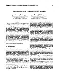
For SA the diamond property holds for the single-step relation, from which the diamond property for the transitive closure easily follows. On the other hand, it is almost obvious that the diamond property cannot hold for λv -calculus. The βv -reduction can copy redexes in the argument of a function, which prevents the existence of the common contractum in certain diamonds. For an example, consider the expression ((λx.(x x)) (λy.((λx.x) (λx.x)))), which contains the two overlapping and underlined βv -redexes. By reducing either one of them we get the expressions ((λx.(x x)) (λy.(λx.x))) and ((λy.((λx.x) (λx.x))) (λy.((λx.x) (λx.x)))). While both expressions contain redexes, the diagram in Figure 2.2 shows that the onestep reductions starting from these expressions do not lead to a common expression. Hence, the one-step relation does not satisfy the diamond property.

((λx.(xx))(λy.((λx.x)(λx.x)))) H ©© HH © H HH ©© j ¼ © ((λy.((λx.x)(λx.x))) ((λx.(xx))(λy.(λx.x))) (λy.((λx.x)(λx.x)))) ¡HH H ¡ HH ? ¡ HH ¡ HH ((λy.(λx.x)) ¡ H (λy.(λx.x)) HH ª ¡ ? j (λy.((λx.x) (λx.x)))

((λy.(λx.x)) (λy.((λx.x)(λx.x))))

((λy.((λx.x)(λx.x)))) (λy.(λx.x))

Figure 2.2: A Failure of the Diamond Property for Onestep v Reductions Since the problem of the one-step relation based on v is caused by reductions that multiply redexes, it is quite natural to consider an extension of the one-step reduction that contracts several non-overlapping redexes in parallel. If this extension satisfies the diamond property and its transitive-reflexive closure is the same as that of the one-step relation, then we should be able to prove the diamond theorem for the v-reduction.


40

The parallel closure of v, notation: Definition 2.5.4 (Parallel v-reduction: −→ −→ 1 ) , is a superset of v such that −→ −→ 1 1. M −→ −→ M; 1 2. (o b1 . . . bn ) −→ −→ δ(o, b1 , . . . , bn ) if δ is defined on o and b1 , . . . , bn ; 1 3. ((λx.M ) U ) −→ −→ N [x ← V ] if M −→ −→ N and U −→ −→ V (for all x ); 1 1 1 4. (M M 0 ) −→ −→ (N N 0 ) if M −→ −→ N and M 0 −→ −→ N 0; 1 1 1 5. (λx.M ) −→ −→ (λx.N ) if M −→ −→ N; 1 1 0 ) if for all i , M −→ 6. (o M1 . . . Mm ) −→ −→ (o M10 . . . Mm Mi0 . i −→ 1 1

And indeed, the parallel reduction does satisfy the diamond property. Lemma 2.5.5 (Diamond Property for −→ −→ 1 ) Let L, M , and N be SA expressions. If L −→ −→ M and L −→ −→ N then there exists an expression K such that M −→ −→ K and 1 1 1 K. N −→ −→ 1 Proof. The proof is an induction on the tree structure of the proof that L −→ −→ M and 1 proceeds by case analysis on the last step in this proof: L = M : Set K = N . (o b1 . . . bn ) −→ −→ δ(o, b1 , . . . , bn ): Since δ is a function there is no other possible reduc1 tion for L, i.e., L = N = M . ((λx.L0 ) U ) −→ −→ M 0 [x ← V ] because L0 −→ −→ M 0 , U −→ −→ V : There are two possiblities 1 1 1 for the second reduction path. Either the two parts of the application reduce separately or the application also reduces the βv -redex: ((λx.L0 ) U ) −→ −→ ((λx.Y 0 ) W ) because L0 −→ −→ N 0 , U −→ −→ W : In this case, L0 , M 0 , 1 1 1 0 and N satisfy the antecedent of the hypothesis and so do U, V , and W . Hence, there are expressions K 0 and X that complete the upper half of these two diamons. If we also knew that substitution and parallel reduction commute, we could conclude that K = K 0 [x ← X] was the desired expression because then ((λx.N 0 ) W ) −→ −→ K 0 [x ← X] and M 0 [x ← V ] −→ −→ K 0 [x ← X]. 1 1 ((λx.L0 ) U ) −→ −→ N 0 [x ← W ] because L0 −→ −→ N 0 , U −→ −→ W : As in the first sub1 1 1 0 0 0 case, L , M , and N and U, V , and W determine upper halves of diamonds, respectively. By induction hypothesis, each yields two lower halves of diamonds and related terms K 0 and X. And again, if substitution and parallel reduction commute, setting K = K 0 [x ← X] concludes the subcase.

2.5. CONSISTENCY

41

To complete this case, we are obliged to prove the commutation property. We postpone this proof since other cases also depend on it: see Lemma 2.5.6. −→ (M1 M2 ) because Li −→ −→ Mi : This case is symmetric to the previous case. (L1 L2 ) −→ 1 1 The proof of the preceding case can easily be adapted. (o L1 . . . Lm ) −→ −→ (o M1 . . . Mm ) because Li −→ −→ Mi for 1 ≤ ileqm: Two cases: 1 1 1. L1 , . . . , Lm are basic constants, N is the δ-contractum of L. Then M = L and K = N. 2. N = (o N1 . . . Nm ) An n-fold use of the inductive hypothesis yields the conclusion. −→ (λx.M 0 ) because L0 −→ −→ M 0 : First, it is clear that N = (λx.N 0 ). Second, (λx.L0 ) −→ 1 1 the induction hypothesis applies to L0 , M 0 , and N 0 and yields an expression K 0 so that we can set K = (λx.K 0 ). To finish the preceding proof, we need to show that substitutions in expressions that are related by parallel reduction do not affect the reduction step. N and U −→ −→ V then M [x ← U ] −→ −→ N [x ← V ]. Lemma 2.5.6 If M −→ −→ 1 1 1 Proof. The proof is an induction on M and proceeds by case analysis on the last step N: in the proof of M −→ −→ 1 M = N : In this special case, the claim says that if U −→ −→ −→ 1 V then M [x ← U ]−→ 1 M [x ← V ]. The proof of this specialized claim is an induction on the structure of M . It proceeds in the same manner as the proof Lemma 2.4.2. M = (o b1 . . . bn ), N = δ(o, b1 , . . . , bn ): Here, M and N are closed, so M [x ← U ] = M , N [x ← V ] = N . The result follows by the assumption of the case. M = ((λy.K) W ), N = L[y ← W 0 ] because K −→ −→ L, W −→ −→ W 0 : A simple calculation 1 1 shows that the claim holds: M [x ← U ]

=

((λy.K[x ← U ]) W [x ← U ])

−→ −→ 1

L[x ← V ][y ← W 0 [x ← V ]]

=

L[y ← W 0 ][x ← V ]

=

N [x ← V ]

(†)

Equation (†) is a basic property of the substitution function. We leave this step as an exercise.


42

−→ Ni : By the induction hypothesis, Mi [x ← M = (M1 M2 ), N = (N1 N2 ) because Mi −→ 1 U ] −→ −→ N [x ← V ] for both i = 1 and i = 2. Thus, i 1 M [x ← U ]

=

(M1 [x ← U ] M2 [x ← U ])

−→ −→ 1

(N1 [x ← V ] N2 [x ← V ])

=

(N1 N2 )[x ← V ]

=

N [x ← V ]

0 ) because M −→ Ni : The proof of this case is M = (o M1 . . . Mm ), N = (o M10 . . . Mm i −→ 1 an appropriate adaptation of that of the previous case.

M = (λx.K), N = (λx.L) because K −→ −→ L: The proof of this case is an appropriate 1 adaptation of that of the previous case. Exercise 2.5.1 Complete Case 1 of Lemma 2.5.6. Exercise 2.5.2 Prove that if y 6∈ FV (L) then K[x ← L][y ← M [x ← L]] = K[y ← M ][x ← L]. (Recall that M = N means M =α N .)

2.6

Observational Equivalence: The Meaning of Equations

Besides program evaluation the transformation of programs plays an important role in the practice of programming and programming language implementation. For example, if M is a procedure and we think that N is a procedure that can perform the same computation as M but faster, then we would like to know whether M is really interchangeable with N . For one special instance of this problem, the λv -calculus clearly provides a solution: If both expressions were programs and we knew M =v N , then eval v (M ) = eval v (N ) and we know that we can replace M by N . In general, however, M and N are sub-expressions of some program, and we may not be able to evaluate them independently. Hence, what we really need is a general relation that explains when expressions are “equivalent in functionality”. To understand the notion of “equivalent in functionality”, we must recall that the user of a programm can only observe the output and is primarily interested in the output. He usually does not know the text of the program or any aspects of the text. In other words, such an observer treats programs as black boxes that magically produce some value. It is consequently natural to say that the effect of an expression is the effect it has when it is a part of a program. Going even further, the comparison of two open

2.6. OBSERVATIONAL EQUIVALENCE: THE MEANING OF EQUATIONS

43

expressions reduces to the question whether there is a way to tell apart the effects of the expressions. Or, put positively, if two expressions have the same effect, they are interchangeable from the standpoint of an external observer. Definition 2.6.1 (Observational Equivalence) Two expressions, M and M 0 , are observationally equivalent, written: M 'v M 0 , if and only if they are indistinguishable in all contexts C such that C[M ] and C[M 0 ] are programs, eval v (C[M ]) = eval v (C[M 0 ]).

Observational equivalence obviously extends program equivalence: If programs M and N are observationally equivalent, then they are programs in the empty context and eval v (M ) = eval v (N ). But this is also the least we should expect from a theory of expressions with equivalent functionality. In addition, and as the name already indicates, observational equivalence is an equivalence relation. Finally, if two expressions are observationally equivalent, then embedding the expresssions in contexts should yield observationally equivalent expressions. After all, the added pieces are identical and should not affect the possible effects of the expressions on the output of a program. In short, observational equivalence is a congruence relation. Proposition 2.6.2 For all ISWIM expressions K, L, M, 1. M 'v M ; 2. if L 'v M and M 'v N then L 'v N ; 3. if L 'v M then M 'v L; and 4. if M 'v N then C[M ] 'v C[N ] for all contexts C . Proof. Points 1 through 3 are trivial. As for point 4, assume M 'v N and let C 0 [ ] be an arbitrary context such that C 0 [C[M ]] and C 0 [C[N ]] are programs. Then, C 0 [C[ ]] is a program context for M and N . By assumption M 'v N and therefore, eval v (C 0 [C[M ]]) = eval v (C 0 [C[N ]]), which is what we had to prove. It turns out that observational equivalence is the largest equivalence relation, that is, the one that equates the most expressions, and still satisfies the general criterion that we outlined above. Proposition 2.6.3 Let ≡ be a congruence relation such that M ≡ N for programs M, N implies eval v (M ) = eval v (N ). If M ≡ N then M 'v N .

44


Proof. We assume M 6'v N and show M 6≡ N . By assumption there exists a separating context C . That is, C[M ] and C[N ] are programs but eval v (C[M ]) 6= eval v (C[N ]). Therefore, C[M ] 6≡ C[N ]. But now by the assumptions about the congruence relation, M 6≡ N . The proposition shows that observational equivalence is the most basic, the most fundamental congruence relation on expressions. All other relations only approximate the accuracy with which observational equivalence identifies expressions. It also follows from the proposition that the λv -calculus is sound with respect to observational equivalence. Unfortunately, it is also incomplete, that is, the calculus cannot prove all observational equivalence relations. Theorem 2.6.4 (Soundness, Incompleteness) If λv ` M = M 0 then M 'v M 0 . The inverse direction does not hold. Proof. By definition, λv is a congruence relation. Moreover, eval v is defined based on λv such that if λv ` M = N and both are programs, then eval v (M ) = eval v (N ). For the inverse direction, we give a counter-example and sketch the proof that it is a counter-example. Consider the expressions (Ω (λx.x)) and Ω. Both terms diverge and are observationally equivalent. But both reduce to themselves only and therefore cannot be provably equal in λv . To complete the proof of the Incompleteness Theorem, we still lack some tools. We will return to the proof in the next chapter, when we have developed some basic more knowledge about the calculus.

Notes Landin: design of iswim Plotkin: design and analysis of iswim calculus Curry: good treatment of substitution Despite claims to the contrary in the literature, na¨ıve substitution does not capture the notion of dynamic binding in Lisp. Cartwright [] offers an explanation. Barendregt: comprehensive study of Church’s λ-calculus as a logical system; numerous techniques applicable to this calculus though the book does not cover lcal as a calculus for a programming language conventions on treatment of terms!

Chapter 3

Standard Reduction The definition of the ISWIM evaluator via an equational proof system is elegant and flexible. A programmer can liberally apply the rules of the equational system in any order and at any place in the program. He can pursue any strategy for such a calculation that he finds profitable and can switch as soon as a different one appears to yield better results. For example, in cases involving the fixed point operator, the right-toleft direction of the βv -axiom is useful whereas in other cases the opposite direction is preferable. However, this flexibility of the calculus is clearly not a good basis for implementing the evaluator eval v as a computer program. Since we know from the Church-Rosser Theorem that a program is equal to a value precisely when it reduces to a value, we already know that we can rely on reductions in the search for a result. But even the restriction to reductions is not completely satisfactory because there are still too many redexes to choose from. An implementation would clearly benefit from knowing that picking a certain reduction step out of the set of possible steps guaranteed progress; otherwise, it would have to search along too many different reduction paths. The solution of the problem is to find a strategy that reduces a program to an answer if it is equal to one. In other words, given a program, it is possible to pick a redex according to a fixed strategy such that the reduction of this redex brings the evaluation one step closer to the result if it exists. The strategy is known as Curry-Feys Standardization. The strategy and its correctness theorem, the Curry-Feys Standard Reduction Theorem, are the subject of the first section. The standard reduction strategy basically defines a textual machine for ISWIM. In contrast to a real computer, the states of a textual machine are programs, and the machine instructions transform programs into programs. Still, the textual machine provides the foundation for a first implementation of the evaluator. A systematic elimination of inefficiencies and overlaps naturally leads to machines with more efficient representations of intermediate states. Every step in this development is easy to justify and to formalize. Another use of the textual machine concerns the analysis of the behavior of pro45

CHAPTER 3. STANDARD REDUCTION

46

grams. For example, all program evaluations either end in a value, continue for ever, or reach a stuck state due to the misapplication of a primitive. Similarly, if a closed subexpression plays a role during the evaluation, it must become the “current” instruction at some point during the evaluation. Background Reading: Plotkin, Felleisen & Friedman

3.1

Standard Reductions

Even after restricting our attention to reductions alone, it is not possible to build a na¨ıve evaluator because there are still too many choices to make. Consider the following program: (((λxy.y) (λx.((λz.zzz) (λz.zzz)))) d 7e ). Both underlined sub-expressions are redexes. By reducing the larger one, the evaluation process clearly makes progress. After the reduction the new program is ((λy.y) d 7e ), which is one reduction step away from the result, d 7e . However, if the evaluator were to choose the inner redex and were to continue in this way, it would not find the result of the program: ((λxy.y) (λx.((λz.zzz) (λz.zzz))) d 7e ) −→v ((λxy.y) (λx.((λz.zzz) (λz.zzz) (λz.zzz)))) d 7e ) −→v ((λxy.y) (λx.((λz.zzz) (λz.zzz) (λz.zzz) (λz.zzz)))) d 7e ) −→v . . . The problem with the second strategy is obvious: it does not find the result of the program because it reduces sub-expressions inside of λ-abstractions but leaves the outer applications of the program intact. This observation also hints at a simple solution. A good evaluation strategy based on reductions should only pick redexes that are outside of abstractions. We make this more precise with a set of two rules: 1. If the expression is an application and all components are values, then, if the expression is a redex, it is the next redex to be reduced; if not, the program cannot have a value. 2. If the expression is an application but does not only consist of values, then pick one of the non-values and search for a potential redex in it. The second rule is ambiguous because it permits distinct sub-expressions of a program to be candidates for further reduction. Since a deterministic strategy should pick a unique sub-expression as a candidate for further reduction, we arbitrarily choose to search for redexes in such an application from left to right:

3.1. STANDARD REDUCTIONS

47

20 . If the program is an application such that at least one of its sub-expressions is not a value, pick the leftmost non-value and search for a redex in there. By following the above algorithm we divide a program into an application consisting of values and a context. The shape of such a context is determined by our rules: it is either a hole, or it is an application and the sub-context is to the right of all values. Since these contexts play a special role in our subsequent investigations, we provide a formal definition. Definition 3.1.1 (Evaluation Contexts) The set of evaluation contexts is the following subset of the set of ISWIM contexts: E ::= [ ] | (V E) | (E M ) | (o V . . . V E M . . . M ) where V is a value and M is an arbitrary expression. To verify that our informal strategy picks a unique sub-expression from a program as a potential redex, we show that every program is either a value or it is a unique evaluation context filled with an application that solely consists of values. Lemma 3.1.2 (Unique Evaluation Contexts) Every closed ISWIM expression M is either a value, or there exists a unique evaluation context E such that M = E[(V1 V2 )] or M = E[(on V1 . . . Vn )] where V1 , . . . , Vn are values. Proof. The proof proceeds by induction on the structure of expressions. If M is not a value, it must be an application. Assume that it is a primitive application of the shape: (on N1 . . . Nn ) where N1 , . . . , Nn are the arguments. If all arguments are values, i.e., Ni ∈ Vals, we are done. Otherwise there is a leftmost argument expression, say Ni for some i, 1 ≤ i ≤ n, that is not a value. By inductive hypothesis, the expression Ni can be partitioned into a unique evaluation context E 0 and an application of the right shape, say L. Then E = (on N1 . . . Ni−1 E 0 Ni+1 . . . Nn ) is an evaluation context and M = E[L]. The context is unique since i is the minimal index such that N1 , . . . , Ni−1 ∈ Vals and E 0 is unique by inductive hypothesis. The case for arbitrary applications proceeds analoguously. It follows from the lemma that if M = E[L] where L is an application consisting of values then L is uniquely determined. If L is moreover a βv or a δ redex, it is the redex that according to our intuitive rules 1 and 20 must be reduced. Reducing it produces a new program, which can be decomposed again. In short, to get an answer for a program: if it is a value, there is nothing to do, otherwise decompose the program into an evaluation context and a redex, reduce the redex, and start over. To formalize this idea, we introduce a special reduction relation.


48

Definition 3.1.3 (Standard Reduction Function) The standard reduction function maps closed non-values to expressions: M 7−→v N iff for some E, M ≡ E[M 0 ], N ≡ E[N 0 ], and (M 0 , N 0 ) ∈ v. We pronounce M 7−→v N as “M standard reduces to N .” As usuall, M 7−→∗v N means M reduces to N via the transitive-reflexive closure of the standard reduction function.

By Lemma 3.1.2 the standard reduction relation is a well-defined partial function. Based on it, our informal evaluation strategy can now easily be cast in terms of standard reduction steps: a program can be evaluated by standard reducing it to a value. Theorem 3.1.4 (Standard Reduction) For any program M , M −→ −→v U for some ∗ −→v U . In particular, if value U if and only if M 7−→v V for some value V and V −→ U ∈ BConsts then M −→ −→v U if and only if M 7−→∗v U . One way to exploit this theorem is to define an alternative evaluator. The alternative eval function maps a program to the normal form of the program with respect to the standard reduction relation, if it exists. Definition 3.1.5 (eval sv ) The partial function eval sv : Λ0 −→ A is defined as follows: ½ b if M 7−→∗v b s eval v (M ) = closure if M 7−→∗v λx.N

It is a simple corollary of Theorem 3.1.4 that this new evaluator function is the same as the original one. Corollary 3.1.6 eval v = eval sv Proof. Assume eval v (M ) = b for some b ∈ BConsts. By Church-Rosser and the fact that constants are normal-forms with respect to v, M −→ −→v b. By Theorem 3.1.4, M 7−→∗v b and thus, eval sv (M ) = b. Conversely, if eval sv (M ) = b then M 7−→∗v b. Hence, M =v b and eval v (M ) = b. A similar proof works for the case where eval v (M ) = closure = eval sv (M ). In summary, (M, b) ∈ eval v if and only if (M, b) ∈ eval sv . Proof of the Standard Reduction Theorem The proof of the Standard Reduction Theorem requires a complex argument. The difficult part of the proof is clearly the left to right direction since the right to left direction is implied by the fact that the standard reduction function and its transitive-reflexive closure are subsets of the reduction relation proper. A na¨ıve proof attempt could proceed by induction on the


49

number of one-step reductions from M to U . Asssume the reduction sequence is as follows: M = M0 −→v M1 −→v . . . −→v Mm = U. For m = 0 the claim vacuously holds, but when m > 0 the claim is impossible to prove by the simple-minded induction. While the inductive hypothesis says that for −→v U there exists a value V such that M1 7−→∗v V , it is obvious that for many M1 −→ pairs M0 , M1 it is not the case that M0 7−→∗v M1 . For example, the reduction step from M0 to M1 could be inside of a λ-abstraction and the abstraction may be a part of the final answer. The (mathematical) solution to this problem is to generalize the inductive hypothesis and the theorem. Instead of proving that programs reduce to values if and only if they reduce to values via the transitive closure of the standard reduction function, we prove that there is a canonical sequence of reduction steps for all reductions. To state and prove the general theorem, we introduce the notion of a standard reduction sequence. A standard reduction sequence generalizes the idea of a sequence of expressions that are related via the standard reduction function. In standard reduction sequences an expression can relate to its successor if a sub-expression in a λ-abstraction standard reduces to another expression. Similarly, standard reduction sequences also permit incomplete reductions, i.e., sequences that may not reduce a redex inside of holes of evaluation context for the rest of the sequence. Definition 3.1.7 (Standard Reduction Sequences) The set of standard reduction sequences is a set of expression sequences that satisfies the following four inductive conditions: 1. Every basic constant b ∈ BConsts is a standard reduction sequence. 2. Every variable x ∈ Vars is a standard reduction sequence. 3. If M1 , . . . , Mm is a standard reduction sequence, then so is λx.M1 , . . . , λx.Mm . 4. If M1 , . . . , Mm and N1 , . . . , Nn are standard reduction sequences, then so is (M1 N1 ), (M2 N1 ), . . . , (Mm N1 ), (Mm N2 ), . . . , (Mm Nn ). 5. If Mi,1 , . . . , Mi,mi are standard reduction sequences for 1 ≤ i ≤ m and mi ≥ 1 then (om M1,1 M2,1 . . . Mm,1 ), (om M1,2 M2,1 . . . Mm,1 ), ..., (om M1,m1 M2,1 . . . Mm,1 ), (om M1,m1 M2,2 . . . Mm,1 ), ..., (om M1,m1 M2,M2 . . . Mm,mm ) is a standard reduction sequence.


50

6. If M1 , . . . , Mm is a standard reduction sequence and M0 7−→v M1 , then M0 , M1 , . . . , Mm is a standard reduction sequence.

Clearly, the standard reduction sequences consisting of a single term are all ISWIM expressions. We can now formulate the claim that is provable using a reasonably simple induction argument. The general idea for such a theorem is due to Curry and Feys, who proved it for Church’s pure λ-calculus. Theorem 3.1.8 (Plotkin) M −→ −→v N if and only if there is a standard reduction sequence L1 , . . . , Ll such that M = L1 and N = Ll . Proof. From right to left, the claim is a consequence of the fact that if K precedes L in a standard reduction sequence then K reduces to L, a property that obviously follows from the definition. To prove the left-to-right direction, assume M −→ −→v N . By the definition of the reduction relation, this means that there exist expressions M1 , . . . , Mm such that M −→v M1 −→v . . . −→v Mm −→v N. The critical idea is now the following: Since the parallel reduction relation extends the one-step relation, it is also true that M1 −→ −→ . . . −→ −→ Mm −→ −→ N. M −→ −→ 1 1 1 1 Moreover, such a sequence of parallel reduction steps can be transformed into a standard reduction sequence, based on the algorithm in the proof of Lemma 3.1.10. The proof of the main lemma relies on a size function for derivations of parallel reductions, that is, the argument that two terms are in the parallel reduction relation. The size of such derivations is approximately the number of v-redexes that an ordinary reduction between terms would have had to perform. Definition 3.1.9 (Size of M −→ −→ 1 N ) The size of the derivation that M parallel reduces to N , M −→ −→ N , is defined inductively according to the last derivation step and the 1 size of subderivations:

3.1. STANDARD REDUCTIONS M −→ −→ M 1 (o b1 . . . bn ) −→ −→ δ(o, b1 , . . . , bn ) 1 (λx.M )U −→ −→ N [x ← V ] 1 because M −→ −→ N is of size sM 1 U −→ −→ V is of size sU 1 (M N ) −→ −→ (M 0 N 0 ) 1 because M −→ −→ M 0 is of size sM 1 N −→ −→ N 0 is of size sN 1 0 ) (o M1 . . . Mm ) −→ −→ (o M10 . . . Mm 1 because Mi −→ −→ Mi0 is of size sMi 1 (λx.M ) −→ −→ (λx.N ) 1 because M −→ −→ N is of size sM 1

51 0 1 sM + #(x, N ) × sU + 1

sM + sN

Σm i=1 sMi

sM

#(x, M ) denotes the number of free x in M . Now we are ready to prove the main lemma. Lemma 3.1.10 If M −→ −→ 1 N and N, N2 , . . . , Nn is a standard reduction sequence, then there is a standard reduction sequence L1 , . . . , Ll such that M = L1 and Ll = Nn . Proof. The proof is a lexicographic induction on the length of the given standard N and the structure of M . It reduction sequence (n), the size of the derivation M −→ −→ 1 proceeds by case analysis on the last step in the derivation of M −→ −→ N: 1 M = N : This case is trivial. M = (o b1 . . . bm ), N = δ m (f, b1 , . . . , bm ): A δ-step that transforms the outermost application is also a standard reduction step. By combining this with the standard reduction sequence from N to Nn yields the required standard reduction sequence from M to Nn . L, U −→ −→ V : M is also a βv -redex, M = ((λx.K) U ), N = L[x ← V ] because K −→ −→ 1 1 which as in the previous case, implies that a βv -step from M to K[x ← U ] is a standard reduction step. By the assumptions and Lemma 2.5.6, the latter expression also parallel reduces to L[x ← V ]. Indeed, we can prove a stronger version of Lemma 2.5.6, see Lemma 3.1.13 below, that shows that the size of this derivation is strictly smaller than the size of the derivation of ((λx.K) U ) −→ −→ 1 L[x ← V ]. Thus, the induction hypothesis applies and there must be a standard

52

CHAPTER 3. STANDARD REDUCTION reduction sequence L2 , . . . , Ll such that K[x ← U ] = L2 and Ll = Nn . Since M 7−→v K[x ← U ], the expression sequence M, L2 , . . . , Ll is the required standard reduction sequence.

M = (M 0 M 00 ), N = (N 0 N 00 ) because M 0 −→ −→ N 0 , M 00 −→ −→ N 00 : Since the standard re1 1 duction sequence N, N2 , . . . , Nn could be formed in two different ways, we must consider two subcases. N 7−→v N2 : This case relies on the following Lemma 3.1.11, which shows that N and N 7−→v N2 then there exists an expression K such that if M −→ −→ 1 M 7−→v K and K −→ −→ −→ 1 N2 . Now, K −→ 1 N2 and N2 , N3 , . . . , Nn is a standard reduction sequence that is shorter than the original one. Hence, by the induction hypothesis there exists a standard reduction sequence L2 , . . . , Ll such that K = L2 and Ll = Nn . Moreover, M 7−→v K, and hence M, L2 , . . . , Ll is the desired standard reduction sequence. otherwise: N 0 , . . . , Nk0 and N 00 , . . . , Nj00 are standard reduction sequences such that N, N2 , . . . , Nn is identical to (N 0 N 00 ), . . . , (Nk0 N 00 ), (Nk0 N200 ), . . . , (Nk0 Nj00 ). By the assumptions and the induction hypothesis, which applies because M 0 and M 00 are proper subterms of M , there exist standard reduction sequences L01 , . . . , L0l1 and L001 , . . . , L00l2 such that M 0 = L01 and L0l1 = Nk0 and M 00 = L001 and L00l2 = Nj00 . Clearly, these two sequences form a single reduction sequence L1 , . . . , Ll such that L1 = (L01 L001 ) = (M 0 M 00 ) and Ll = (L0l1 L00l2 ) = (Nk0 Nj00 ) = Nn , which is precisely what the lemma demands. 0 )becauseM −→ M = (o M1 . . . Mm ), N = (o N10 . . . Nm Ni : Again, the standard reduci −→ 1 tion sequence starting at N could be the result of two different formation rules. The proofs in both subcases though are completely analoguous to the two subcases in the previous case so that there is no need for further elaboration.

M = (λx.K), N = (λx.L) because K −→ −→ L: By the definition of standard reduction 1 sequences, all of the expressions Ni are λ-abstractions, say, Ni = λx.Ni0 . Hence, K −→ −→ L and L, N20 , . . . , Nn0 is a standard reduction sequence. Since K is a 1 proper sub-expression of M , the induction hypothesis applies and there must be a standard reduction sequence L01 , . . . , L0l such that K = L01 and L0l = Nn0 . By taking Li = λx.L0i , we get the desired standard reduction sequence. These are all possible cases and we have thus finished the proof. Lemma 3.1.11 If M −→ −→ N and N 7−→v L then there exists an expression N ∗ such 1 −→ L. that M 7−→∗v N ∗ and N ∗ −→ 1 Proof. The proof is a lexicographic induction on the size of the derivation of M −→ −→ 1 N and the structure of M . It proceeds by case analysis on the last step in the parallel reduction derivation.


53

M = N : In this case, the conclusion vacuously holds. M = (o b1 . . . bm ), N = δ m (o, b1 , . . . , bm ): Since the result of a δ-step is a value, it is impossible that N standard reduces to some other term. L, U −→ −→ V : M is also a βv -redex, M = ((λx.K) U ), N = L[x ← V ] because K −→ −→ 1 1 and therefore M 7−→v K[x ← U ]. Next, by Lemma 2.5.6 L[x ← V ], K[x ← U ] −→ −→ 1 and the derivation of this parallel reduction is smaller than the derivation of M −→ −→ 1 N by Lemma 3.1.13. By induction hypothesis, there must be an expression −→ L[x ← V ]. Hence we can prove the desired N ∗ such that K[x ← U ] 7−→v N ∗ −→ 1 conclusion as follows: M 7−→v K[x ← U ] 7−→v N ∗ −→ −→ L[x ← V ]. 1 −→ N 0 , M 00 −→ −→ N 00 : Here we distinguish M = (M 0 M 00 ), N = (N 0 N 00 ) because M 0 −→ 1 1 three subcases according to the standard reduction step from N to L: N = ((λx.K 0 ) N 00 ) where N 00 ∈ Values: That is, N is a βv -redex and L is its contractum. By the assumed parallel reductions and Lemma 3.1.12 below, there exist (λx.K) and N ∗∗ such that M 0 7−→∗v (λx.K) −→ −→ (λx.K 0 ) and 1 00 ∗∗ 00 ∗ M 7−→v N −→ −→ N . Hence, 1 (M 0 M 00 ) 7−→∗v ((λx.K) M 00 ) 7−→∗v ((λx.K) N ∗∗ ) 7−→v K[x ← N ∗∗ ] −→ −→ 1

K 0 [x ← N 00 ],

which is precisely what the lemma claims. N = (E[K] N 00 ): Then, L = (E[K 0 ] N 00 ) where (K, K 00 ) ∈ v and −→ E[K] 7−→E [K 0 ]. M 0 −→ 1 By the induction hypothesis, which applies because M 0 is a proper subexpression of M , this means that there exists an expression N1∗ such that −→ E[K 0 ], M 0 7−→∗v N1∗ −→ 1 which implies that −→ (E[K 0 ] N 00 ). (M 0 M 00 ) 7−→∗v (N1∗ M 00 ) −→ 1 In other words, N ∗ = (N1∗ M 00 ).


54

N = (N 0 E[K]) and N 0 ∈ Values: In this case, L = (N 0 E[K 0 ]) where (K, K 00 ) ∈ v and −→ E[K] 7−→E [K 0 ]. M 00 −→ 1 The induction hypothesis again implies the existence of an expression N2∗ such that −→ E[K 0 ]. M 00 7−→∗v N2∗ −→ 1 Since M 0 may not be a value, we apply the following lemma to get a value N1∗ such that −→ N 0. M 0 7−→∗v N1∗ −→ 1 Putting it all together we get, (M 0 M 00 ) 7−→∗v (N1∗ M 00 ) 7−→∗v (N1∗ N2∗ )

7−→v (N1∗ N2∗ ) −→ −→ 1

(N 0 E[K 0 ]).

And thus, N ∗ = (N1∗ N2∗ ) in this last subcase. 0 )becauseM −→ M = (o M1 . . . Mm ), N = (o N10 . . . Nm Ni : The proof is analoguous to i −→ 1 the preceding one though instead of a βv step the first subcase is a δ-step. That is, all Ni0 are basic constants and N standard reduces to a value. Since Lemma 3.1.12 shows that a term that parallel reduces to a basic constant also standard reduces to it, the rest of the argument is straightforward.

L: This case is again impossible because the M = (λx.K), N = (λx.L) because K −→ −→ 1 standard reduction function is undefined on values. This completes the case analysis and the proof. Lemma 3.1.12 Let M be an application. ∗ −→ 1. If M −→ −→ 1 (λx.N ) then there exists an expression λx.L such that M 7−→v (λx.L)−→ 1 (λx.N ).

N where N = x or N = c then M 7−→∗v N . 2. If M −→ −→ 1 Proof. Both implications follow from an induction argument on the size of the derivation for the parallel reduction in the antecedent. 1. Only a parallel δ or a parallel βv reduction can transform an application into a λ-abstraction. Clearly, δ reductions are also standard reductions and therefore the result is immediate in this case. Parallel βv redexes are standard redexes.


55

Thus, M = ((λy.M 0 ) U ), which parallel reduces to (λx.N ) = N 0 [y ← V ] because −→ N 0 and U −→ −→ V by Lemma 2.5.6. Hence, M 0 −→ 1 1 −→ N 0 [y ← V ] = λx.N. ((λy.M 0 ) U ) 7−→v M 0 [y ← U ] −→ 1 By Lemma 3.1.13, we also know that the latter derivation is shorter than the original parallel reduction step and therefore, by inductive hypothesis, ((λy.M 0 ) U ) 7−→v M 0 [y ← U ] 7−→∗v N. 2. Again, the only two parallel reductions that can transfrom a redex in the shape of an application into a constant or variable are δ and the βv (parallel) reductions. Thus the argument proceeds as for the first part. Lemma 3.1.13 If M −→ −→ N has size sM and U −→ −→ V has size sN then (i) M [x ← 1 1 U ] −→ −→ N [x ← V ] and (ii) size s of the derivation of the latter is less than or equal to 1 sM + #(x, N ) × sU . Remarks: (1) This lemma is a strengthening of Lemma 2.5.6. For completeness, we repeat the proof of the original lemma and add components about the size of the parallel reduction derivation. (2) The lemma implies that the size of the derivation of ((λx.M ) U ) −→ −→ N [x ← V ] is 1 strictly larger than the size of the derivation of M [x ← U ] −→ −→ N [x ← V ]. 1 Proof. The proof is an induction on M and proceeds by case analysis on the last step in the derivation of M −→ −→ N: 1 −→ M = N : In this special case, the claim says that if U −→ −→ 1 V then M [x ← U ]−→ 1 M [x ← V ]. As to the claim about size: the assumption implies that sM = 0, and therefore it must be true that s ≤ #(x, M ) × sU . The derivation of this specialized claim is an induction on the structure of M :

M = c: M [x ← U ] = c −→ −→ c = M [x ← V ]; 1 size: s = 0; V = M [x ← V ]; M = x: M [x ← U ] = U −→ −→ 1 size: s = sU = #(x, M ) × sU ; y = M [x ← V ]; M = y 6= x: M [x ← U ] = y −→ −→ 1 size: s = 0; (λy.K[x ← V ]) = M [x ← V ] by M = (λy.K): M [x ← U ] = (λy.K[x ← U ]) −→ −→ 1 induction hypothesis for K ; size: s = #(x, K) × sU = #(x, M ) × sU ;


56

(K[x ← V ] L[x ← V ]) = M = (K L): M [x ← U ] = (K[x ← U ] L[x ← U ]) −→ −→ 1 M [x ← V ] by induction hypothesis for K , L; size: s = #(x, K) × sU + #(x, L) × sU = #(x, M ) × sU . M = (o b1 . . . bm ), N = δ(o, b1 , . . . , bm ): Here, M and N are closed, so M [x ← U ] = M , N [x ← V ] = N , and the result follows directly from the assumption. Size: s = 0. M = ((λy.K) W ), N = L[y ← W 0 ] because K −→ −→ L, W −→ −→ W 0 : A simple calculation 1 1 shows that the claim holds: M [x ← U ]

substitution lemma

=

((λy.K[x ← U ]) W [x ← U ])

−→ −→ 1

L[x ← V ][y ← W 0 [x ← V ]]

=

L[y ← W 0 ][x ← V ]

=

N [x ← V ]

(†)

Equation (†) follows from a simple induction on the structure of L. The size of the derivation is calculated as follows. Let us assume the following conventions about sizes: sK : s0K : sW : s0W :

K −→ −→ L 1 K[x ← U ] −→ −→ L[x ← V ] 1 0 W −→ −→ W 1 W [x ← U ] −→ −→ W 0 [x ← V ] 1

By induction hypothesis, s0K

s0W

≤ sK + #(x, L) × sU

≤ sW + #(x, W 0 ) × sU

Hence, the size for the entire derivation is s = s0K + #(y, L) × s0W + 1

≤ sK + #(x, L) × sU + #(y, L) × (sW + #(x, W 0 ) × sU ) + 1

= sK + #(y, L) × sW + 1 + (#(y, L) × #(x, W 0 ) + #(x, L)) × sU = sM + #(x, N ) × sU

M = (M1 M2 ), N = (N1 N2 ) because Mi −→ −→ Ni : By the induction hypothesis, Mi [x ← 1 U ] −→ −→ Ni [x ← V ] for both i = 1 and i = 2. Thus, 1 M [x ← U ]

=

(M1 [x ← U ] M2 [x ← U ])


57 −→ −→ 1

(N1 [x ← V ] N2 [x ← V ])

=

(N1 N2 )[x ← V ]

=

N [x ← V ]

For the size argument, we again begin by stating some conventions: −→ Ni si : Mi −→ 1 0 si : Mi [x ← U ] −→ −→ Ni [x ← V ] 1 Thus, by induction hypothesis, s0i ≤ si + #(x, Ni ) × sU . The rest follows from a simple calculation: s = s01 + s02 ≤ s1 + #(x, N1 ) × sU + s2 + #(x, N2 ) × sU = s1 + s2 + (#(x, N1 ) + #(x, N2 )) × sU = sM + #(x, N ) × sU

0 )becauseM −→ M = (o M1 . . . Mm ), N = (o N10 . . . Nm Ni : The proof of this case proi −→ 1 ceeds as the preceding one.

L: The proof of this case is also an approM = (λx.K), N = (λx.L) because K −→ −→ 1 priate adaptation of the proof for the application case. These are all possible cases and we have thus finished the proof. First, it

The reward of proving the standard reduction theorem is a proof of Theorem 3.1.4, provides a powerful tool the correctness proof for the textual machine. Theorem 3.1.4 For any program M , M −→ −→v U for some value U if and only if ∗ M 7−→v V for some value V and V −→ −→v U . In particular, if U ∈ BConsts then M −→ −→v U if and only if M 7−→∗v U . Proof. To prove the left to right direction, assume that M −→ −→v U and that M is not a value. It follows from the Standard Reduction Theorem that there exists a standard reduction sequence L1 , . . . , Ll such that M = L1 and Ll = U . By

for proving and disproving equations in the λv -calculus. Second, we can now show that evaluation is indeed equivalent to standard reduction steps.


58

induction on the length of the sequence, there exists an index i such that Li is the first value in the sequence and M = L1 7−→∗v Li . −→v U . Moreover, constants can only be the end of a standard Set V = Li ; trivially, Li −→ reduction sequence of values if the standard reduction sequence is a singleton. Hencem the second part of the theorem concerning basic constants obviously holds. In summary, we have now shown that the specification of the evaluation function based on the equational system is equivalent to an evaluator based on the standard reduction function. Since the latter is a truly algorithmic specification, we can now implement the evaluator easily. Exercise 3.1.1 Implement the standard reduction function 7−→v as a procedure standard that maps ISWIM programs to ISWIM programs. Implement eval sv based on the standard . Pick some simple benchmarks and determine their running time on the machine. Hint: Make sure that the computations in the test programs do not dominate the execution of the transition function.

3.2 need to say that the machines are functions

Machines

Every evaluation cycle in our textual machine performs three steps: 1. It tests whether the program is a value; if so, the machine stops. 2. If the program is an application, the machine partitions the program into an evaluation context, E , and an application, (U V ) or (o V1 . . . Vm ), whose subterms are values. 3. If the application is a βv or δ redex, the machine constructs the contractum M and fills the evalutaion context E with the contractum M . The result of such a step is the program E[M ], which is the next machine state. Now the evaluation cycle starts over. An obvious problem with this machine is the repeated partitioning of a program into an evaluation context and a redex. Clearly, the evaluation context of the (n + 1)st step is often the same as, or at least, is closely related to the one for the nth step. For example, consider the evaluation of (1+ ((λx.((λy.((λz.x) d 3e )) d 2e )) d 1e )),

3.2. MACHINES

59

which is a fairly typical example: (1+ ((λx.((λy.((λz.x) d 3e )) d 2e )) d 1e )) 7−→v (1+ ((λy.((λz.d 1e ) d 3e )) d 2e )) 7−→v (1+ ((λz.d 1e ) d 3e )) 7−→v (1+ d 1e ) 7−→v

d e

2.

The redexes in each intermediate state are underlined, the evaluation context is the part of the term that is not underlined. The evaluation context for the first three states is (1+ [ ]). But the machine has to recompute the evaluation context at every stage.

3.2.1

The CC Machine

The appropriate method for dealing with this repeated computation is to separate states into the “current subterm of interest” and the “current” evaluation contexts. Putting the former into the hole of the latter yields the complete program. We will refer to the “term of interest” as the control string and the evaluation contexts simply as contexts. The machine is appropriately called CC machine. In addition to the tasks of the textual machine, the CC machine is responsible for searching the next redex. Initially only the entire program can be the control string; the initial evaluation context must be the empty context. The search instructions implement rules 1 and 20 from the beginning of this chapter. That is, if the control string is not an application that consists of values, the leftmost non-value becomes the control string, the rest becomes a part of the evaluation context. For example, if the control string is ((M N ) L) and the evaluation context is E[ ], then the machine must search for the redex in (M N ) and must remember the shape of the rest of the program. Consequently the next state of the machine must have (M N ) as the control string component and must refine the current context E[ ] to a context of the shape E[([ ] L)]. Put succinctly, the CC machine must have a state transition of the form h(M N ), E[ ]i 7−→ hM, E[([ ] N )]i if M 6∈ Vals. Search rules for other shapes of applications that do not solely consist of values are needed, too. Once the control string becomes a redex, the CC machine must naturally simulate the actions of the textual machine to be a faithful implementation. Thus it must have the following two instructions: h(o b1 . . . bm ), E[ ]i 7−→ hV, E[ ]i where δ(o, b1 , . . . , bm ) = V h((λx.M )V ), E[ ]i − 7 → hM [x ← V ], E[ ]i

(cc.δ) (cc.β)


60

The result of one of these transitions might be a state that pairs a value with an evaluation contexts. In the textual machine this corresponds to a step of the form E[R] 7−→v E[V ]. Now the textual machine would actually divide the second program into a redex R0 and an evaluation context E 0 [ ] that is distinct from E[ ]. But the textual machine clearly does not pick random pieces from the evaluation context to form the next redex. If E[ ] = E ∗ [((λx.M ) [ ])] then E 0 [ ] = E ∗ [ ] and R0 = ((λx.M ) V ), that is, the new redex is formed of the innermost application in E[ ], and E 0 [ ] is the rest of E[ ]. For a faithful simulation of the textual machine, the CC machine needs a set of instructions that exploit the information surrounding the hole of the context when the control string is a value. In the running example, the CC machine would have to make a transition from hV, E ∗ [((λx.M ) [ ])]i to h((λx.M ) V ), E ∗ []i. Now the control string is an application again, and the search process can start over. Putting it all together, the evaluation process on a CC machine consists of shifting pieces of the control string into the evaluation context such that the control string becomes a redex. Once the control string has turned into a redex, an ordinary contraction occurs. If the result is a value, the machine must shift pieces of the evaluation context back to the control string.

Definition 3.2.1 (CC machine) State space: Λ0 × EConts

3.2. MACHINES

61

State transitions: Redex h(M N ), E[ ]i if M 6∈ Vals h(V M ), E[ ]i if M 6∈ Vals h(o V1 . . . Vi M N . . .), E[ ]i if M 6∈ Vals, for all i ≥ 0 h((λx.M ) V ), E[ ]i h(o b1 . . . bm ), E[ ]i

Contractum 7 → hM, E[([ ] N )]i −

cc 1

7−→ hM, E[(V [ ])]i

2

7−→ hM, E[(o V1 . . . Vi [ ] N . . .)]i

3

− 7 → hM [x ← V ], E[ ]i 7−→ hV, E[ ]i where δ(o, b1 , . . . , bm ) = V hV, E[(U [ ])]i 7−→ h(U V ), E[ ]i hV, E[([ ] N )]i 7−→ h(V N ), E[ ]i hV, E[(o V1 . . . Vi [ ] N . . .)]i 7−→ h(o V1 . . . Vi V N . . .), E[ ]i

βv δv

The evaluation function: eval cc v (M )

½ =

b closure

4 5 6

if hM, [ ]i 7−→∗cc hb, [ ]i if hM, [ ]i − 7 →∗cc hλx.N, [ ]i

By the derivation of the CC machine, it is almost obvious that it faithfully implements the textual machine. Since evaluation on both machines is defined as a partial function from programs to answers, a formal justification for this claim must show that the two functions are identical. The following theorem formulates this idea and proves it. Theorem 3.2.2 eval sv = eval cc v s Proof. We need to show that if (M, a) ∈ eval cc v then (M, a) ∈ eval v and vice versa. By the definition of the two evaluation functions, this require a proof that

M 7−→∗v V if and only if hM, [ ]i 7−→∗cc hV, [ ]i. A natural approach to the proof of this claim is an induction of the length of the given transition sequence. However, since intermediate states have non-empty evaluation contexts in the context component, we will need a slightly stronger induction hypothesis: For all evaluation contexts E[ ], terms M , and values V , E[M ] 7−→∗v V if and only if hM, E[ ]i 7−→∗cc hV, [ ]i.


62

The hypothesis clearly implies the general theorem. Thus the rest of the proof is a proof of this intermediate claim. The proof for each direction is an induction on the length of the reduction sequence. To prove the left to right direction of the claim, assume E[M ] 7−→∗v V . If the reduction sequence is empty, the conclusion is immediate, so assume there is at least one step: E[M ] 7−→v E 0 [N ] 7−→∗v V where (L, N ) ∈ v for some L. By inductive hypothesis, hN, E 0 [ ]i 7−→∗cc hV, [ ]i. To conclude the proof, we must show that hM, E[ ]i 7−→cc hN, E 0 [ ]i. Depending on the shape of M and E[ ], there are four possibilities: M = E 00 [L]: Then, E 0 [ ] = E[E 00 [ ]]. By Lemma 3.2.3 below, hM, E[ ]i 7−→∗cc hL, E[E 00 [ ]]i and, hence, by a (cc.δ) or (cc.βv ) transition, hL, E[E 00 [ ]]i − 7 →cc 00 hN, E[E [ ]]i. E[ ] = E 0 [((λx.N 0 ) [ ])], M ∈ Vals: A first step puts the redex into the control position, which enables a (cc.βv ) reduction: hM, E 0 [((λx.N 0 ) [ ])]i 7−→cc h((λx.N 0 ) M ), E 0 [ ]i 7−→cc hN 0 [x ← M ], E 0 [ ]i. Since the assumptions imply that N = N 0 [x ← M ], this proves the conclusion. E[ ] = E 00 [([ ] K)], M ∈ Vals: Depending on the nature of K , there are two different scenarios: 1. If K ∈ Values then L = (K M ), which implies the conclusion. 2. If K 6∈ Values then there exists an evaluation context E 000 [ ] such that K = E 000 [L]. Hence, E 0 [] = E 00 [(M E 000 [L])] and hM, E 00 [([ ] K)]i 7−→cc h(M K), E 00 [ ]i 7−→cc hK, E 00 [(M [ ])]i 7−→∗cc hL, E 00 [(M E 00 [ ])]i by Lemma 3.2.3 7−→∗cc hN, E 00 [(M E 00 [ ])]i =

hN, E 0 [ ]i.

E[ ] = E 0 [(o b1 . . . [ ] . . . bn )], M ∈ BConsts: Appropriate adaptations of the proofs of the second and third case prove the conclusion.

3.2. MACHINES

63

For the right to left direction, assume hM, E[ ]i 7−→∗cc hV, [ ]i. The proof is a again an induction on the number of transition steps. If there are none, M ∈ Vals and E[ ] =, which implies the claim. Otherwise, there is a first transition step: hM, E[ ]i 7−→cc hN, E 0 [ ]i 7−→∗cc hV, [ ]i. By inductive hypothesis, E 0 [N ] 7−→∗v V . The rest of the proof depends on which kind of transition the CC-machine made to reach the state hN, E 0 [ ]i. If the first transition was one of (cc.1), . . . , (cc.6), then E[M ] = E 0 [N ], and the conclusion follows. If it is a (cc.βv ) or a (cc.δ) transition, then E[M ] 7−→v E 0 [N ]. Put together with the inductive hypothesis, E[M ] 7−→v E 0 [N ] 7−→∗v V. Lemma 3.2.3 For all evaluation contexts E[ ], if M = E 0 [L] and L is a v-redex, then hM, E[ ]i 7−→∗cc hL, E[E 0 [ ]]i. Proof. The proof is an induction on the structure of E 0 . If E 0 [ ] = [ ] then the conclusion is immediate. Otherwise, E 0 [ ] has one of the following three shapes: E 0 [ ] = (E 00 [ ] N ), E 0 [ ] = (V E 00 [ ]), or E 0 [ ] = (o V1 . . . Vn E 00 [ ] N . . .). In each case, the machine can move the pieces surrounding E 00 [ ] to the context component, e.g., h(E 00 [L] N ), E[ ]i 7−→cc hE 00 [L], E[([ ] N )]i. Since E 00 [ ] is a component of E 0 [ ], the conclusion follows from the inductive hypothesis. Exercise 3.2.1 Implement the CC-transition function 7−→cc that maps CC-states to CC-states. Implement evaluation contexts as an extension of ISWIM expressions. Define eval cc v based on the transition function. Benchmark the same programs that you used for the test of eval sv (see Exercise 1). Explain the timings.

3.2.2

Simplified CC Machine

The CC machine faithfully immitates the textual machine by performing all of the work on the control string. Consider the following example: ((λx.x) ((λx.x) d 5e )), consisting of an application of two applications, which evaluates as follows: h((λx.x) ((λx.x) d 5e )), [ ]i 7−→cc h((λx.x) d 5e ), ((λx.x) [ ])i 7−→cc hd 5e , ((λx.x) [ ])i


64

At this point, the CC-machine is forced to construct an application such that one of the application rules can put the second application in the control string register: . . . 7−→cc h((λx.x) d 5e ), [ ]i 7−→cc hd 5e , [ ]i. The next to last step is only needed because the CC machine only exploits information in the control string position. One way to simplify the CC-machine is to combine the rules for values with the reduction of redexes such that the last two steps become one step. A similar simplification is possible when the value returned belongs into the function position. A simple variation of the first example shows how the machine again moves information into the control string even though the next step is clear: h(((λx.x) (λx.x)) ((λx.x) d 5e )), [ ]i 7−→cc h((λx.x) (λx.x)), ([ ] ((λx.x) d 5e ))i 7−→cc h(λx.x), ([ ] ((λx.x) d 5e ))i. Now the machine constructs an application only to move on to the evaluation of the argument expression: 7−→cc h((λx.x) ((λx.x) d 5e )), [ ]i 7−→cc h((λx.x) d 5e ), ((λx.x) [ ])i ... Instead of constructing the application, the machine could always put the argument into the control register and put the value for the function position into the evaluation context. If the argument is a value, the modified machine can perform a reduction. If not, the current CC machine would have reached this state, too. Once we have a machine that combines the recognition of a value with the reduction of a redex, when possible, we can also omit the specialized treatment of applications. The current CC machine has three distinct transitions for dealing with applications and three more for dealing with primitive applications. Side-conditions ensure that only one transition applies to any given application. These separate rules are only necessary because the machine performs all the work on the control string and uses the control stack only as a simple memory. Together with the perviously suggested simplifications, we can eliminate the side-conditions, the reduction rules, and the rule cc.2, which only exists to move arguments from evaluation contexts into the control start calling string position. things registers The simplified CC machine has fewer transitions and no side-conditions. Given a state finding the applicable transition rule is easy. If the control string is an application, shift a fixed portion to the evaluation context and concentrate on one sub-expression. If it is a value, check the innermost application of the evaluation context. If the hole is in the last position of the application, perform a reduction, otherwise swap information between the control string register and the evaluation context register.

3.2. MACHINES

65

Definition 3.2.4 (Simplified CC machine) State space: Λ0 × EConts State transitions: Redex h(M N ), E[ ]i h(o M N . . .), E[ ]i hV, E[((λx.M ) [ ])]i hV, E[([ ] N )]i hb, E[(o b1 . . . bi [ ])]i

Contractum scc hM, E[([ ] N )]i 1 hM, E[(o [ ] N . . .)]i 2 hM [x ← V ], E[ ]i 3 hN, E[(V [ ])]i 4 hV, E[ ]i 5 where δ(o, b1 , . . . , bi , b) = V hV, E[(o V1 . . . Vi [ ] N L . . .)]i 7−→ hN, E[(o V1 . . . Vi V [ ] L . . .)]i 6

The evaluation function: eval scc v (M )

7 → − 7−→ 7−→ 7−→ 7−→

½ =

b closure

if hM, [ ]i 7−→∗scc hb, [ ]i if hM, [ ]i 7−→∗scc hλx.N, [ ]i

The CC machine and the simplified version define the same evaluation function. scc Theorem 3.2.5 eval cc v = eval v

Proof. The proof of this theorem is analoguous to the proof of Theorem 3.2.2. That is, unfolding the definition of the two evaluation functions leads to the proof obligation that hM, [ ]i 7−→∗cc hV, [ ]i if and only if hM, [ ]i 7−→∗scc hV, [ ]i. The correct stregthening of this claim to an inductive hypothesis extends it to arbitrary intermediate states: For all evaluation contexts E[ ], terms X, and values V , hM, E[ ]i 7−→∗cc hV, [ ]i if and only if hM, E[ ]i 7−→∗scc hV, [ ]i. The key idea for the proof of the intermediate claim is that for any given program, the CC-machine and the SCC-machine quickly synchronize at some state provided the initial state leads to a result. More precisely, given hM, E[ ]i such that E[M ] = E 0 [L] and L is a v-redex, there exists a state hN, E 00 []i such that 00 + 00 hM, E[ ]i 7−→+ cc hN, E []i and hM, E[ ]i 7−→scc hN, E []i.

By definition, M is either a value or an expression that contains a redex. Moreover, if M is a value, the evaluation context must contain an innermost application: E[ ] = E 0 [(o V1 . . . Vm [ ]N1 . . . Nn )], E[ ] = E 0 [(V [ ])], or E[ ] = E 0 [([ ] N )]. Hence, the initial state hM, E[ ]i falls into one of the following four possibilities:


66

M = E 0 [L]: The CC-machine evaluates the initial state as follows: hE 0 [L], E[ ]i 7−→∗cc hL, E[E 0 [ ]]i 7−→cc hN, E[E 0 [ ]]i. The SCC machine eventually reaches the same state, but the intermediate states depend on the shape of the redex L. If L = ((λx.L0 ) L00 ), then the SCC-machine reaches hL00 , E[E 0 [((λx.L0 ) [ ])]]i as the next to last state; otherwise, the next to last state is hb, E[E 0 [(o b1 . . . bi [ ])]]i where L = (o b1 . . . bi b). M ∈ V als, E[ ] = E 0 [((λx.L0 ) [ ])]: Here the CC-machine creates a redex in the control component and reduces it: hM, E 0 [((λx.L0 ) [ ])]i 7−→cc h((λx.L0 ) M ), E 0 []i 7−→cc hL0 [x ← M ], E 0 []i. The SCC-machine avoids the first step and immediately goes into the same state. M ∈ V als, E[ ] = E 0 [([ ] N )]: If N ∈ V als, the proof of this case proceeds along the lines of the second case. Otherwise, hM, E 0 [([ ] N )]i 7−→cc h(M N ), E 0 [ ]i, 7−→cc hN, E 0 [(M [ ])]i. Again, the SCC-machine skips the intermediate state. M ∈ V als, E[ ] = E 0 [(o V1 . . . Vm [ ] N1 . . . Nn )]: The transition sequences depend on the shape of the sequence N1 , . . . , Nn . There are three possible cases: 1. If the sequence N1 , . . . , Nn is empty, M, V1 , . . . , Vm must be basic constants and δ(o, V1 , . . . , Vm , V ) = U for some value U . It follows that hM, E 0 [(o V1 . . . Vn [ ])]i 7−→cc h(o V1 . . . Vn M ), E 0 [ ]i 7−→cc hU, E 0 [ ]i. As in the previous case, the SCC-machine reaches the final state by skiping the intermediate state. 2. If N1 , . . . , Nn is not empty but N1 , . . . Nn ∈ Vals, then hM, E 0 [(o V1 . . . Vm [ ] N1 . . . Nn )]i 7−→cc h(o V1 . . . Vm M N1 . . . Nn ), E 0 [ ]i 7−→cc hU, E 0 [ ]i. Now, the SCC-machine needs to perform a number of additional steps, which serve to verify that the additional arguments are values: hM, E 0 [(o V1 . . . Vm [ ] N1 . . . Nn )]i 7−→scc hN1 , E 0 [(o V1 . . . Vm M [ ] N2 . . . Nn )]i 7−→∗scc . . .

7−→∗scc hNn , E 0 [(o V1 . . . Nn−1 [ ])]i 7−→scc hU, E 0 [ ]i.

3.2. MACHINES

67

3. If N1 , . . . , Nn is not empty and Ni 6∈ Vals then both machines reach the intermediate state hNi , E 0 [(o V1 . . . Vn N1 . . . Ni−1 [ ] Ni+1 . . .)]i after an appropriate number of steps. The rest of the proof is a straightforward induction on the number of transition steps. Assume hM, E[ ]i 7−→∗cc hV, [ ]i. If M = V, E[ ] = [ ], the conclusion is immediate. Otherwise, E[M ] must contain a redex since the machine reaches a final state. By the above, there must be an intermediate state hN, E 0 [ ]i that both machines reach after some number of steps. By the inductive hypothesis, both machines also reach hV, [ ]i from this intermediate state. The proof of the opposite direction proceeds in the same fashion. Exercise 3.2.2 Implement the SCC-transition function 7−→cc as a procedure standard that maps SCC-states to SCC-states. Implement eval scc v . Check whether the simplified machine is faster or slower on your benchmarks.

3.2.3

CK Machine

Any description of an evaluation on the CC or simplified CC machine refers to the innermost application of the evaluation context. That is, the application that directly contains the hole. When the control string is an application, a new innermost application is created. When the control string turns into a value, the next step is determined by considering this innermost application. In short, the transitions always access the evaluation context from the inside and in a last-in, first-out fashion. Transition steps depend on the precise shape of the first element but not on the rest of the data structure. The observation suggests that the evaluation context register should be a list of applications with a hole: K ::= Ks∗ Ks ::= (V [ ]) | ([ ] N ) | (o V . . . V [ ] N . . .) For readability and for ease of implementation, we tag each case of this construction and invert the list of values in a primitive application: K ::=

mt | hfun, V, Ki | harg, N, Ki | hnarg, hV, . . . , V, oi, hN, . . .i, Ki

This data structure is called a continuation code.


68 Definition 3.2.6 (CK machine) State space:

Λ0 × KCodes

where the set KCodes is defined by the grammar: K ::=

mt | hfun, V, Ki | harg, N, Ki | hnarg, hV, . . . , V, oi, hN, . . .i, Ki

State transitions: Redex h(M N ), Ki h(o M N . . .), Ki hV, hfun, (λx.M ), Kii hV, harg, N, Kii hb, hnarg, hbi . . . b1 oi, hi, Kii

Contractum ck hM, harg, N, Kii 1 hM, hnarg, hoi, hN, . . .i, Kii 2 hM [x ← V ], Ki 3 hN, hfun, V, Kii 4 hV, Ki 5 where δ(o, b1 , . . . , bi , b) = V hN, hnarg, hV, V 0 , . . .i, hL, . . .i, Kii 6

7−→ 7−→ 7−→ 7−→ 7−→

hV, hnarg, hV 0 . . . oi, hN, L, . . .i, Kii 7−→ The evaluation function: eval ck v (M )

½ =

b closure

if hM, mti 7−→∗ck hb, mti if hM, mti 7−→∗ck hλx.N, mti

Given an SCC-state it is trivial to find a corresponding CK-state and vice versa based on a bijection between the set of evaluation contexts and the set of continuation codes: KC : KCodes  −→ EvalConts [ ]    0 E [([ ] N )] KC(K) = E 0 [(V [ ])]    0 E [(o V1 . . . Vi [ ] N . . .)] where E 0 [ ] = KC(K 0 )

if if if if

K K K K

= mt = harg, N, K 0 i = hfun, V, K 0 i = hnarg, hVi , . . . , V1 , oi, hN, . . .i, K 0 i

CK : EvalConts  −→ KCodes mt    hfun, N, K 0 i CK(E[ ]) = harg, V, K 0 i    hnarg, hVi , . . . , V1 , oi, hN, . . .i, K 0 i where K 0 = CK(E 0 [ ])

if if if if

E[ E[ E[ E[

]=[ ] ] = E 0 [([ ] N )] ] = E 0 [(V [ ])] ] = E 0 [(o V1 . . . Vi [ ] N . . .)]

3.2. MACHINES

69

Based on this bijection between CC and CK states, it is easy to prove the correctness of the evaluation function based on the CK machine. ck Theorem 3.2.7 eval scc v = eval v

Proof. Based on the translations between states, it is easy to check that 1. if hM, E[ ]i 7−→scc hN, E 0 [ ]i then hM, CK(E[ ])i 7−→ck hN, CK(E 0 [ ])i; 2. if hM, Ki 7−→ck hN, K 0 i then hM, KC(K)i 7−→scc hN, KC(K 0 )i. By trivial inductions on the length of the transition sequences, it follows that hM, [ ]i 7−→∗scc hV, [ ]i if and only if hM, mti 7−→∗ck hV, mti, which implies the theorem. Exercise 3.2.3 Modify the SCC-transition function 7−→cc of exercise 2 into an implescc mentation of the CK-transition function. Measure the speed-up of eval ck v over eval v .

3.2.4

CEK Machine

Starting with the textual machine, the reduction of a βv -redex requires the substitution of a value for all occurrences of an identifier. When the result of the substitution operation is not a value, it becomes the control string until it is reduced to a value. Then the machine traverses many of the applications that the substituition operation just traversed. To avoid this repeition of work, we delay the substitution until needed. That is, every expression in the machine is replaced by a pair whose first component is an open term and whose second component is a function that maps all free variables to their correponding expressions. The pair is called a closure and the function is an environment. Of course, environments cannot map varibales to expressions because this would re-introduce expressions into the machine, but must map variables to closures. Definition 3.2.8 (Environments; Closures) The sets of environments and closures are defined by mutual induction: 1. An environment is a finite function from variables to value closures. If x1 , . . . , xn are distinct variables and cl 1 , . . . , cl n are value closures (for n ≥ 0), then {hx1 , cl1 i, . . . , hxn , cln i} is an environment. Given E = {x1 , . . . , xn }, E(xi ) = cli and E ’s domain, written: Dom(E) is {x1 , . . . , xn }.


70

2. Let M be an ISWIM expression and let E be an environment such that FV (M ) ⊆ Dom(E). Then, hM, Ei is a closure. If M ∈ Values, then it is a value closure. If E is an environment and x a variable, then shadowing x in E, notation: E \ x, yields the environment that is like E but lacks a definition for x : df

E \ x ⇔ {hy, E(y)i | y ∈ Dom(E), y 6= x}. If E is an environment, x a variable, and cl a closure, then the update of E at x to cl , notation: E[x ← cl ], yields an environment that now maps x to cl : df

E[x ← cl ] ⇔ (E \ x ) ∪ {hx , cl i}.

Based on the notions of closures and environments, it is easy to reformulate the CK machine into a machine that works on control strings with environments and continuation codes: the CEK machine.

Definition 3.2.9 (The CEK machine) State space: Closures × EKCodes where the set EKCodes of CEK continuation codes is defined by the grammar: K ::=

mt | hfun, vcl, Ki | harg, cl, Ki | hnarg, hv, . . . , v, oi, hcl, . . .i, Ki

with vcl ranging over value closures and cl over closures.

3.2. MACHINES

71

State transitions: Redex hh(M N ), Ei, Ki hh(o M N . . .), Ei, Ki

Contractum 7−→ hhM, Ei, harg, hN, Ei, Kii 7−→ hhM, Ei, hnarg, hoi, hhN, Ei, . . .i, Kii 7−→ hhM, E 0 [x ← hV, Ei]i, Ki

hhV, Ei, hfun, h(λx.M ), E 0 i, Kii if V 6∈ Vars hhV, Ei, harg, N, Kii if V 6∈ Vars hhb, Ei, hnarg, hhbi , Ei i . . . hb1 , E1 i oi, hii, Ki

7−→ hN, hfun, hV, Ei, Kii

7−→ hV, Ki where δ(o, b1 , . . . , bi , b) = V 0 0 hhV, Ei, hnarg, hcl , . . .i, hhN, E i, cl, . . .i, Kii 7−→ hhN, E 0 i, hnarg, hhV, Ei, cl0 , . . .i, hcl, . . .i, Kii if V 6∈ Vars hhx, Ei, Ki 7−→ hcl, Ki where E(x) = cl

cek 1 2 3 4 5 6

7

The evaluation function: ½ eval cek v (M ) =

b closure

if hM, mti 7−→∗ck hb, mti if hM, mti 7−→∗ck hhλx.N , Ei, mti

Given a CEK-state it is again straightforward to find a corresponding CK-state. The basic idea is to replace every closure in the state by the closed term that it represents: unload : Closures −→ Λ0 unload (hM, Ei) = M [x1 ← unload (cl1 )] . . . [xn ← unload (cln )] where E = {hx1 , cl1 i, . . . , hxn , cln i} Since closures also occur inside of CEK-continuation codes, the translation of CEKstates into CK-states requires an additional traversal of CEK-continuation codes to replace these closures: KK : KCodes  −→ EKCodes [ ] if K = mt     if K = harg, cl, K 0 i  harg, unload (cl), K ∗ i if K = hfun, cl, K 0 i hfun, unload (cl), K ∗ i KK(K) =  0 ∗  hnarg, hunload (cl ), . . . oi, hunload (cl), . . .i, K i    if K = hnarg, hcl0 , . . . oi, hcl, . . .i, K 0 i where K ∗ = KK(K 0 )


72

Unfortunately it is impossible to define inverses of these functions: given a closed term, there are many closures that map back to the same term. As a result, the simple proof method of the preceding adequacy theorems for verifying the equality between the SCC-evaluator and the CK-evaluator fails here. However, as in the preceding subsections, it is still the case that the CEK-machine can simulate any given sequence of CK-states if the initial state of the two machines are equivalent. cek Theorem 3.2.10 eval ck v = eval v

Proof. Given the translation from CEK-states it is easy to check that for any intermediate state hcl, Ki in the sequence of CEK-states, there is a state hcl0 , K 0 i such that hcl, Ki 7−→∗ck hcl0 , K 0 i and

hunload (cl), KK(K)i 7−→ck hunload (cl0 , KK(K 0 ))i.

Hence, hhM, ∅i, mti 7−→∗ck hhV, Ei, mti implies hM, mti 7−→ck hunload (hV, Ei), mt)i, which proves the right-to-left direction. The left-to-right direction requires a stronger induction hypothesis than the rightto-left direction or the inductions of the preceding adequacy theorems because of the lack of a function from CK-states to CEK-states. In addition to the intial state of the transition sequence of the CK-machine, we need to know the initial state of the CEK-machine: For every CK-state hM1 , K1 i and CEK-state hhM10 , Ei, K10 i such that M1 = unload (hM10 , Ei) and K1 = KK(K10 ), if hM1 , K1 i 7−→∗ck hV, mti then for some closure cl with unload (cl) = V , hhM10 , Ei, K10 i 7−→∗ck hcl, mti. The theorem follows from specializing the two initial states to hM, mti and hhM, ∅i, mti. The proof of the claim is by induction on the length of the transition sequence in the CK-machine. It proceeds by case analysis of the initial state of the CK-machine: M1 = (L N ): The CK-machine performs a (ck.1) instruction: h(L N ), K1 i 7−→ck hL, harg, N, K1 ii. By assumption, hM10 , Ei = h(L0 N 0 ), Ei such that L = unload (hL0 , Ei) and N = unload (hN 0 , Ei) since unload preserves the shape of applications in the translation process. Hence, hh(L0 N 0 ), Ei, K10 i 7−→ck hhL0 , Ei, harg, hN 0 , Ei, K10 ii. Clearly, KK(harg, hN 0 , Ei, K10 i) = harg, N, K1 i. Thus the inductive hypothesis applies and proves the claim for this case.

3.2. MACHINES

73

M1 ∈ Values, K1 = hfun, (λx.N ), K2 i: Here the CK-transition sequence begins as follows: hM1 , hfun, (λx.N ), K2 ii 7−→ck hN [x ← M1 ], K2 i. Given the definition of unload , there are two kinds of CEK-states that can map to the given CK-state: M10 6∈ Vars: Here the CEK-step directly corresponds to the CK-step: hhM10 , Ei, hfun, h(λx.N ), E 0 i, K2 ii 7−→ck hhN, E 0 [x ← hM10 , Ei]i, K2 i. M10 ∈ Vars, unload (E(M10 )) = M1 : If the value is a variable, the CEK-machine first looks up the value of the variable in the environment before it performs an appropriate transition: hhM10 , Ei, hfun, h(λx.N 0 ), E 0 i, K2 ii 7−→ck E(M10 ), hfun, h(λx.N ), E 0 i, K2 i 7−→ck hhN, E 0 [x ← E(M10 )]i, K2 i.

In both cases, the assumptions state unload (hM10 , Ei) = M1 . Hence, to finish the case, we must show that unload (hN 0 , E 0 [x ← cl]i) = N [x ← unload (cl)] where cl = hM10 , Ei. From the definition of unload , if E = {hx1 , cl1 i, . . . , hx1 , cl1 i}, unload (hλx.N 0 , E 0 i) = λx.N 0 [x1 ← unload (cl1 )] . . . [xn ← unload (cln )] = λx.N, which implies N 0 [x1 ← unload (cl1 )] . . . [xn ← unload (cln )] = N. By the Substitution Lemma,

subst lemma

N [x ← unload (cl)] = N 0 [x1 ← unload (cl1 )] . . . [xn ← unload (cln )][x ← unload (cl)] = unload (hN 0 , E[x ← cl]i). The rest follows again by induction on the length of the CK-transition sequence. The proof of the other cases are analoguous to preceding one. Exercise 3.2.4 Implement the CEK-transition function and the CEK-evaluator. Measure the speed-up of eval cek over eval ck v v . Exercise 3.2.5 Choose a concrete representation for the environment component, e.g., a stack, and introduce instructions for extending environments and looking up values.


74

3.3

The Behavior of Programs

The Standard Reduction Theorem is also useful for the analysis of the behavior of programs.

3.3.1

Observational Equivalence

Two expressions are of the same kind if both are values or both are applications (nonvalues). Lemma 3.3.1 (Activity Lemma) Let M be a closed expression and let C be a context. If eval v (C[M ]) exists, then (i) either eval v (C[M 0 ]) exists for all closed expressions M 0 that are of the same kind as M ; or (ii) for all closed expressions M 0 that are of the same kind as M , there is some evaluation context E such that (a) if M is an application, then C[M 0 ] 7−→∗v E[M 0 ]; (b) if M is a λ-abstraction, then for some value U , C[M 0 ] 7−→∗v E[(M 0 U )]; (c) if M is a constant, then for some primitive o and basic constants b1 , . . . , bm , C[M 0 ] 7−→∗v E[(o b1 . . . M 0 . . . bm )]. Proof. Intuitively, the proof proceeds by induction on the number of standard reduction steps in the reduction: C[M ] 7−→∗v V. However, because M may be duplicated during βv -reductions, the induction hypothesis needs to be strengtened. The stronger claim is subject of the following lemma. The formulation of an appropriate induction hypothesis for the Activity Lemma requires the notion of a multi-hole context. Definition 3.3.2 (ISWIM Multi-Hole Contexts) Let [ ]i for all i ∈ N be new members of the alphabet distinct from variables, constants, λ, ., and (, ). The set of multi-hole contexts is a set of ISWIM expressions with some holes: C ::=

[ ]1 | . . . | [ ]i | . . . |M | (C C) | (λx.C) | (on C . . . C)

3.3. THE BEHAVIOR OF PROGRAMS

75

where M ∈ Λ, x ∈ Vars. C, C 0 , and similar letters range over multi-hole contexts. If there is no need to index the holes individually, we use the notation C[·, . . . , ·] to indicate that C ranges over context with m holes.; otherwise, we write C[ ]1 . . . [ ]m . Filling the holes of a multi-hole context is like filling the hole of a single-hole context. The stronger version of the lemma re-states the claim for m expressions and contexts with m holes. Lemma 3.3.3 Let M1 , . . . , Mm be closed expressions and let C be a context with m holes. If eval v (C[M1 , . . . , Mm ]) exists, then 0 ]) for all closed expressions M 0 , . . . , M 0 that are of (i) either eval v (C[M10 , . . . , Mm m 1 the same kind as M1 , . . . , Mm , respectively; or 0 that are of the same kind as M , . . . , M , (ii) for all closed expressions M10 , . . . , Mm 1 m respectively, there is some evaluation context E such that for some i , 1 ≤ i ≤ m,

(a) if Mi is an application, then 0 ] 7−→∗v E[Mi0 ]; C[M10 , . . . , Mm

(b) if Mi is a λ-abstraction, then for some value U , 0 ] 7−→∗v E[(Mi0 U )]; C[M10 , . . . , Mm

(c) if Mi is a constant, then for some primitive o and basic constants b1 , . . . , bm , 0 ] 7−→∗v E[(o b1 . . . M 0 . . . bm )]. C[M10 , . . . , Mm

Proof. The proof is an induction on the number of standard reduction steps for the original program. If C[M1 , . . . , Mm ] is a value, part (i) of the conclusion clearly applies. Consequently, assume that C[M1 , . . . , Mm ] 7−→v K 7−→∗v V for some expression K and value V . By Lemma 3.1.2, the program can be partitioned into an evaluation context E 0 and a redex (P Q) such that E 0 [(P Q)] = C[M1 , . . . , Mm ], or into an evaluation context E 0 and a redex (o c1 . . . cm+1 ) such that E 0 [(o c1 . . . cm+1 )] = C[M1 , . . . , Mm ]. We deal with the first case; the proof of the second case proceeds in an analogous how about the manner: second case?


76

1. Some expression Mi contains, or is equal to, the redex (P Q). Since (P Q) is an application and E 0 an evaluation context, this is only possible if Mi is an application. If this is the case, the first clause of part (ii) of the lemma’s 0 of the correct kind, conclusion holds: for any expressions M10 , . . . , Mm 0 ]m E[ ] = C[M10 ]1 , . . . , [ ]i , . . . , [Mm 0 is an evaluation context. The key to this claim is that the expressions M10 , . . . , Mm are of the same kind as the expressions M1 , . . . , Mm , respectively. If

E 0 [ ] = E1 [(Mj E2 [ ])] where Mj , 1 ≤ j ≤ m, is a value, and E1 and E2 are evaluation contexts, then if Mj0 were an application, E would not be an evaluation context. 2. None of the expressions M1 , . . . , Mm contains the redex, but the redex contains some of these expressions. Now we must consider two subcases: (a) Some λ-abstraction Mi is P . Now the second clause of part (ii) holds: for 0 , all closed expressions M10 , . . . , Mm 0 E[ ] = C[M10 , . . . , [ ]i , . . . Mm ]

and U differs from Q only in occurrences of holes of C. Again, as in the pre0 ceding case, E is an evaluation context because the expressions M10 , . . . , Mm are of the right kind. Similarly, if Q = Mj , for some j , 1 ≤ j ≤ m, then if Mj0 were not a value, U wouldn’t be a value.

(b) The value P is a λ-abstraction, λx.P 0 , that may contain some of the expressions M1 , . . . , Mm . Now: C[M1 , . . . , Mm ] = E 0 [((λx.P 0 ) Q)] 7−→v E 0 [P 0 [x ← Q]]

0 are of the right As in the first subcase, since the expressions M10 , . . . , Mm kind, 0 C[M10 , . . . , Mm ] = E 00 [((λx.P 00 ) Q0 )] 7−→v E 00 [P 00 [x ← Q0 ]]

for some evaluation context E 00 , expression P 00 , and value Q0 that differ accordingly from E 0 , P 0 , and Q respectively. Since the expressions M1 , . . . , Mm are closed, there is some context C 0 of n holes and a sequence of indices 1 ≤ j1 , . . . , jn ≤ m such that E 0 [P 0 [x ← Q]] = C 0 [Mj1 , . . . , Mjn ] and

E 00 [P 00 [x ← Q0 ]] = C 0 [Mj01 , . . . , Mj0n ].

3.3. THE BEHAVIOR OF PROGRAMS

77

The intermediate program satisfies the antecedent of our claim, the reduction C 0 [Mj1 , . . . , Mjn ] 7−→∗v V is shorter, and therefore the induction hypothesis applies. Equipped with the Activity Lemma, we are ready to finish Theorem 2.6.4 with the following lemma. It shows the observational equivalence of two expressions that are not provably equal. Lemma 3.3.4 Ω 'v (Ω (λx.x)) Proof. Let C[ ] be a context such that C[Ω] and C[(Ω (λx.x))] are programs. Assume that eval v (C[Ω]) exists. By the Activity Lemma, it could be the case that for all closed expressions M there is some evaluation context such that C[M ] 7−→∗v E[M ]. But this contradicts the assumption that C[Ω] exists because E[Ω] is a diverging program. Hence, eval v (C[M ]) exists for all closed expressions M and in particular for M = (Ω (λx.x)). Conversely, assume that eval v (C[(Ω (λx.x))]) exists, then by an argument along the same lines, eval v (C[Ω]) exists. Clearly, if one of the programs returns an abstraction, then so does the other, and both return the same basic constant. In short, eval v (C[(Ω (λx.x))]) = eval v (C[Ω]). This proves that Ω 'v (Ω (λx.x)) because C is arbitrary.

3.3.2

Uniform Evaluation

Another question that can now be tackled is the following: what kind of behavior can we expect from a machine given an arbitrary program? The evaluator can diverge for two different reasons. First, every intermediate state of the evaluation may have a successor state. That is, the program is looping. Second, the evaluation may reach an intermediate state for which the standard reduction function is undefined: M1 7−→v M2 7−→v . . . 7−→v Mm such that 7−→v is undefined for Mm and Mm is not an answer. For this to be the case, Mm must contain an application consisting of values in the hole of an evaluation contexts such that neither the βv nor the δ reduction applies, i.e., Mm = E[(U V )] or Mm = E[(o V1 . . . Vn )]

where U is not a basic constant where some Vi is a λ-abstraction or δ(o, V1 , . . . , Vn ) is undefined

some more interesting observationl equivalences? M ' Ω if M is stuck


78

Adopting a machine-oriented view, programs for which 7−→v is undefined are called stuck states. Stuck states play an important role in the analysis of machines and other programming language tools. A precise understanding of the stuck states of any given programming language is therefore crucial. We first give a formal definition of ISWIM stuck states. Definition 3.3.5 (Stuck Applications; Stuck Programs) An application M is stuck if 1. M = (om b1 . . . bm ) iff δ(om , b1 , . . . , bm ) is undefined; or 2. M = (om b1 . . . (λx.N ) . . . bm ); or 3. M = (b V ) (for b ∈ BConsts). A program M is stuck if M = E[N ] for some evaluation context E and a stuck appliction N. Indeed, a program in pure ISWIM can only evaluate to a value, a stuck program, or diverge. Lemma 3.3.6 If M is a program (closed expression), then either 1. M 7−→∗v V for some value V ; 2. M 7−→∗v N for some stuck program N ; 3. for all N such that M 7−→∗v N there exists an L such that N 7−→v L. Proof. Assume there exists an N such that M 7−→∗v N and 7−→v is undefined for N . That is, M1 7−→v M2 7−→v M3 7−→v . . . 7−→v Mm = N. By the Unique Evaluation Context Lemma (Lemma 3.1.2), N is either a value, or there is an evaluation context E[ ], possibly a primitive o, and values U, V, V1 , . . . , Vn such that N = E[(U V )] or N = E[(on V1 . . . Vn )]. If the applications in the hole are redexes, we have a contradiction to our assumption. Consequently, U is neither a λ-abstraction nor a primitive but is a basic constant. Similarly, some Vi must not be a basic constant or δ(on , V1 , . . . , Vn ) is not defined. Hence, N is a stuck program. In conclusion, programs either diverge, or reduce to a Need a lemma value or to a stuck state. that says The following chapter will address a uniform, language-based treatment of stuck beta/delta do states. not introduce free variables

Notes The general idea for such a theorem is due to Curry and Feys [ref: Curry&Feys], who proved it for Church’s pure λ-calculus.

Chapter 4

Functional Extensions and Alternatives 4.1

Complex Data in ISWIM

The set of Cons ISWIM expressions, called Λ, contains the following expressions: M

::=

x | (λx.M ) | (M M ) | b | (on M . . . M ) | (cons M M ) | carM | cdrM

The set of Cons ISWIM values, Vals c ⊆ Λ, is the collection of basic constants (b ∈ BConsts), variables (x ∈ Vars), λ-abstractions in Λ, and pairs of values: V ::= b | x | λx.M | (cons V V ). In addition to V , U, V, W, X also range over values. Also, Vals 0 = {V ∈ Vals | FV (V ) = ∅}. (car (cons V U )) car V (cdr (cons V U )) cdr U Exercise: vectors of values, Exercise: other constructors Question: facilities for defining new constructors?

4.2

Complex Data and Procedures as Recognizable Data

Definition 4.2.1 (Extended δ-function) A δ-function f for the set of function symS bols n∈N FConsts n is a family of partial (n + 1)-ary functions, f n , for each n where 79

CHAPTER 4. FUNCTIONAL EXTENSIONS AND ALTERNATIVES

80

FConsts n 6= ∅, such that f n maps an n-ary functional constant and n basic constants to a closed value: . . × Vals }0 −→ Vals 0 . f n : FConsts n × |Vals 0 × .{z n

If f (o, V1 , . . . , Vn ) does not exist, we also say o is undefined for b1 , . . . , bn . Now definable: number? : Vals −→ Vals procedure? : Vals −→ Vals car : Vals −→ Vals ...

4.3 4.3.1

Call-By-Name ISWIM and Lazy Constructors Call-By-Name Procedures ((λx.M ) N )βM [x ← N ]

Otherwise the song remains the same show that the observational theory is not a sub-theory of the strict theory

4.3.2

Lazy Constructors

The set of Cons ISWIM values, Vals c ⊆ Λ, is the collection of basic constants (b ∈ BConsts), variables (x ∈ Vars), λ-abstractions in Λ, and pairs of values: V ::= b | x | λx.M | (cons M M ). In addition to V , U, V, W, X also range over values. Also, Vals 0 = {V ∈ Vals | FV (V ) = ∅}. (car (cons M N )) car M (cdr (cons M N )) cdr N

Chapter 5

Simple Control Operations An ISWIM program might diverge for two distinct reasons. First, a program’s standard reduction sequence may have a successor for every intermediate state. This situation corresponds to a genuine infinite loop in the program, which, in general, cannot be detected. Second, a program’s standard reduction sequence may end in a stuck state, that is, a program that is not a value and has no successor. One typical example is the application of the division primitive to 0; another one is the use of a numeral in function position. An interpreter that diverges when a program reaches a stuck state leaves the programmer in the dark about the execution of his program. The interpreter should instead signal an error that indicates the source of the trouble. One way to specify the revised interpreter for ISWIM is to add the element “error” to the set of answers and to add a single clause to the definition of the evaluator:  if M 7−→∗v b  b closure if M 7−→∗v λx.N eval (M ) =  error if M 7−→∗v N and N is stuck. By Lemma 3.3.6, which shows that the three enumerated cases plus divergence are the only possible ways for the evaluation of a program to proceed, we know that the extended evaluator is still a partial function from programs to answers. However, beyond programming errors, it is often necessary to terminate the execution of a program in a controlled manner. For example, a program may encode an input-output process for a certain set of data but may have to accept data from some larger set. If the input data for such a program are outside of its proper domain, it should signal this event and terminate in a predictable manner. In plain ISWIM, a programmer can only express the idea of signaling an error by writing down an erroneous expression like (/ d 1e d 0e ). What is needed is a linguistic tool for programmers to express error termination directly. We solve this problem by adding error constructs to the syntax of ISWIM. In the extended language a programmer can 81

CHAPTER 5. SIMPLE CONTROL OPERATIONS

82

explicitly write down “error” with the intention that the evaluation of error terminates the execution of the program. We treat this extended version of ISWIM in the first section of this chapter. Once a language contains constructs for signaling errors it is also natural to add constructs that detect whether an error occurred during the evaluation of a subprogram such that the program can take remedial action. These constructs are highly desirable in practice and are provided by many programming languages. Indeed, these constructs are often used to exit from loops once the result has been detected or to implement some form of backtracking. After examining errors and error handlers, we take a brief look at simple control constructs like try and fail and Lisp’s catch and throw.

5.1

Errors

Since a program can encounter many different types of error situations, we add an undetermined set of errors to ISWIM. Each element of this set plays the role of a syntactic construct. We assume that the set is non-empty but make no other restrictions for now. Definition 5.1.1 (Error ISWIM: Syntax ) Let Errors be a set of terminals that does not overlap with Vars, BConsts, or FConsts, the sets of variables, basic and function constant symbols. The symbol error ranges over the elements of Errors but it is also used as if it were an element of Errors. The set of Error ISWIM expressions, Λe , is the extension of Λ with the elements of Error : M ::= x | (λx.M ) | (M M ) | b | (on M . . . M ) | error

for error ∈ Errors

The notions of context, syntactic compatibility (see Definitions 2.1.2 and 2.1.3, and Proposition 2.1.4) and syntactic equality are adapted mutatis mutandis from Λ.

5.1.1

Calculating with Error ISWIM

Roughly speaking, if a sub-expression raises an error signal, the error should eliminate any computation that would have beeen executed if the evaluation of the sub-expression had not raised an error signal. A precise specification of the behavior of error in terms of calculation rules requires an analysis of how error interacts with other syntactic constructions. Thus, take application as an example. If a function is applied to error, the appliction must be terminated. We can express this with the following informal notions of reduction ((λx.M ) error) −→ error;

(o error) −→ error.

The rule also clarifies that error is not an ordinary value; otherwise applications like ((λx.d 5e ) error) would reduce to d 5e . The case for error in function position is similarly

5.1. ERRORS

83

straightforward. When error occurs in function position, there is no function to be applied so the application also reduces to error: (error M ) −→ error. Next we need to consider the situation when error occurs as the body of a procedure body. Since a procedure like λx.error may never be invoked, the error should not propagate through the abstraction. The hidden error should only become visible when the λ-abstraction is applied to a value. Technically speaking, λx.error is irreducible. Given that the evaluation context surrounding a redex represents the rest of the computation, a natural formalization of the behavior of error says that it erases evaluation contexts. Thus, we introduce the following error reduction: E[error] −→ error

(error)

In addition to occurrences of error in the original program, stuck expressions should now reduce to some error value. Consider the application of some basic constant b to an arbitrary value V . It should reduce to an error that signals that b cannot be used as a procedure: (b V ) −→ errorb . The question is whether the generated error should also depend on the nature of V . Suppose an application of b to U for V 6= U reduces to a distinct error, say, error0b . Then, if it is also the case that V −→ −→ U , the calculus proves errorV = (b V ) = (b U ) = errorU . That is, the two distinct errors are provably equal even though they are not identical and were assumed to be distinct. Implementations of programming languages avoid this problem by signaling an error that only depends on the basic constant in the function position and not on the argument: After all, the argument may actually be the intended one. If the set of errors is rich Following the same reasoning, an application of a primitive operation to a value enough, we can other than a constant must also reduce to an error, independent of the actual argureserve one ments. For example, applying the addition primitive to any abstraction yields the error error per basic constant constant to signal this kind (+ (λxy.x) 0) −→ error+ of error.

and (+ (λxy.y) 0) −→ error+ , independent of the argument. Finally, we need to consider the application of primitive operations to a bad set of basic constants. Since the application is unique and the error message depends on the constant, we demand that the δ functions return appropriate error messages for bad


84

inputs of a function. Thus, the interpretation of good and bad data is combined in a single definition. We can now give a formal definition of the calculus and the evaluator for Error ISWIM . Definition 5.1.2 (The Error ISWIM Calculus and Evaluator ) The set of Error ISWIM values, Vals e , is the collection of basic constants (b ∈ BConsts), variables (x ∈ Vars), and λ-abstractions: V ::= b | x | λx.M. The set of evaluation contexts for Error ISWIM is the following set of contexts: E ::= [ ] | (V E) | (E M ) | (o V . . . V E M . . . M ) where V is a value and M is an arbitrary expression. For Error ISWIM a δ-function f is a family of total (n + 1)-ary functions, f n , for each n where FConsts n 6= ∅, such that f n maps an n-ary functional constant and n basic constants to a closed value or an error element: f n : FConsts n × BConsts × .{z . . × BConsts} −→ Vals 0 ∪ Errors. | n

An application M is faulty if 1. M = (om b1 . . . bm ) and f m (om , b1 , . . . , bm ) ∈ Errors; or 2. M = (om V1 . . . (λx.N ) . . . Vm ); or 3. M = (b V ) (for b ∈ BConsts). The basic notions of reduction for Error ISWIM are: δ : (om b1 . . . bm )δV iff f m (om , b1 , . . . , bm ) = V : Vals 0 βv : ((λx.M ) V )

βv

M [x ← V ]

δerror : Fix an error element errorb for each basic constant b and an error constant erroro for each primitive operation o. Then, M δerror error iff one of the following three conditions holds: • (b V )δerror errorb ; • (om V1 . . . (λx.N ) . . . Vm )δerror erroro ; • (om b1 . . . bm )δerror error iff f m (om , b1 , . . . , bm ) = error. error : E[error] error error

5.1. ERRORS

85

The complete notion of reduction is the union of these relations: e = βv ∪ δ ∪ error ∪ δerror

(e)

The one-step e-reduction −→e is the compatible closure of e. Next, −→ −→e is the e-reduction; it is the reflexive, transitive closure of −→e . Finally, =e is the smallest equivalence relation generated by −→e . If M1 =e M2 , we also write λv -e ` M1 = M2 to emphasize the fact that the calculus is an equational proof system. The set of Error ISWIM answers is the set of basic constants plus the symbols closure and error: A = BConsts ∪ Errors ∪ {closure}. The partial function eval e : Λ0e −→ A is defined   b closure eval e (M ) =  error

as follows: if M =e b if M =e λx.N if M =e error

Next we need to check that the addition of error does not destroy the key properties of the evaluator. To begin with, we would like to know that the evaluator and thus the programming language are still functional. That is, our goal is to establish a consistency theorem for Error ISWIM. Theorem 5.1.3 (Consistency) The relation eval e is a partial function. The proof of this theorem has the same structure as the proof of Theorem 2.5.1, the corresponding theorem for eval v . We first prove a Church-Rosser property, that is, we showq that provably equal results reduce to some common contractum. The theorem follows from Church-Rosser property. The proof of the property relies on the fact that the diamond property holds for the underlying reduction. The diamond property for δ and βv extended to the larger syntax obviously holds; an adaptation of the proof for ISWIM to Error ISWIM is straightforward. But the calculus for Error ISWIM also includes reductions that create and move error. Fortunately, it is possible to combine the diamond theorems for different reductions on the same language, a method that we will use to establish the diamond property for e. We first deal with the extension of the ISWIM calculus to the larger syntax. Let w = δ ∪ βv , i.e., the extension of v to Λe , the full set of Error ISWIM expressions. The notation −→w and −→ −→w denote the one-step reduction and its transitive-reflexive closure, respectively. Lemma 5.1.4 (Diamond Property for −→ −→w ) Let L, M , and N be Error ISWIM expressions. If L −→ −→w M and L −→ −→w N then there exists an expression K such that −→w K. M −→ −→w K and N −→


86

Next we turn to the analysis of the two new notions of reduction. Let f = error ∪ δerror . Unlike v or w, this notion of reduction never duplicates expressions or creates new opportunities to reduce sub-expressions. We should therefore expect that the onestep relation satisfies the diamond property, though unfortunately, it does not hold. Consider the reduction from E[error] to error. If E[error] also reduces to E 0 [error] for some evaluation context E 0 [ ], then E 0 [error] directly reduces to error. Hence it is not the one-step reduction −→f but its reflexive closure −→0f that satisfies the diamond property. Lemma 5.1.5 (Diamond Property for −→ −→f ) Let L, M , and N be Error ISWIM −→f N then there exists an expression K such that expressions. If L −→ −→f M and L −→ M −→ −→f K and N −→ −→f K. Proof. Following the discussion leading up to this lemma, we first prove the claim for a subset of the relation: If L −→0f M and L −→0f N then there exists an expression K such that M −→0f K and N −→0f K. The lemma clearly follows from this claim. The proof proceeds by case analysis of the reduction from L to M : L is faulty; M = error: Clearly, if L is faulty and L −→f N then N is faulty. Hence, K = error is the desired fourth expression. L = E[error]; M = error: It is easy to check that any f-reduction applied to E[error] yields an expression of the shape E 0 [error] for some evaluation context E 0 [ ], which implies that the reduction error applies to N . L = M : Set K = N . L = C[L0 ], M = C[error], (L0 , error) ∈ f : If N = C 0 [L0 ] for some context C 0 [ ], then K = C 0 [error] because C[L0 ] −→f C 0 [L0 ] implies that for all N 0 , C[N 0 ] −→f C 0 [N 0 ]. Otherwise N = C 0 [error] by the definition of compatibility, in which case K = M = N. Exercise 5.1.1 Prove: If L is faulty and L −→f N then N is faulty and reduces to the same error element. Exercise 5.1.2 Prove: If L = E[error] and L −→f M then there exists an evaluation context E 0 [ ] such that M = E 0 [error]. After establishing that each of the notions of reduction w and f on Λe satisfy the diamond property, we need to show that these results can be combined. Intuitively, the combination of w and f should have the diamond property because the two notions

5.1. ERRORS

87

of reduction do not interfere with each other. That is, if two reductions apply to a term, the redexes do not overlap and the reduction of one redex may destroy but not otherwise affect the other redex. Technically speaking, the two one-step reductions commute. −→s be relations on some Definition 5.1.6 (Commuting Reductions) Let −→ −→r and −→ set A. The relations commute if for all a, b, and c, a −→ −→r b

and

a −→ −→s c

and

c −→ −→r d.

implies the existence of d such that b −→ −→s d

If we can show that the one-step relations based on w and f commute, the commutation for their transitive closures clealry follows. However, the one-step relations do not commute. Consider the expression ((λf.(f (f d 0e ))) (λx.(1+ (λx.x)))). Reducing the underlined δerror -redex first yields ((λf.(f (f d 0e ))) (λx.error1+ )) −→e ((λx.error1+ ) ((λx.error1+ ) d 0e )); but reducing the βv -redex first requires two δerror -reductions to reach the same state: ((λx.(1+ (λx.x))) ((λx.(1+ (λx.x))) d 0e )) −→e ((λx.error1+ ) ((λx.(1+ (λx.x))) d 0e )) −→e ((λx.error1+ ) ((λx.error1+ ) d 0e )). Fortunately, it is still possible to extend a commutation result for the one-step relations to the full reductions when only one direction needs multiple steps. The proof of the following lemma illustrates the idea. −→f commute. Lemma 5.1.7 The reductions −→ −→w and −→ Proof. The first step of the proof shows that for all L, M, N ∈ Λe such that L −→w M and L −→f N there exists a K ∈ Λe such that M −→ −→f K and N −→0w K. The proof of the claim is an induction on the derivation of L −→w M : L = ((λx.L0 ) V ), M = L0 [x ← V ]: Only two subcases are possible because a value cannot reduce to error:


88

N = ((λx.L00 ) V ), L0 −→f L00 : If we can show that M [x ← V ] −→f M 0 [x ← V ] if M −→f M 0 , then we can take K = L00 [x ← V ]. N = ((λx.L0 ) V 0 ), V −→f V 0 : If we can show that M [x ← V ] −→ −→f M [x ← V 0 ] if V −→f V 0 , then we can take K = L0 [x ← V 0 ]. LδM : Then, by definition of δ and δerror , it is impossible that L −→f N . L = C[L0 ], M = C[M 0 ], (L0 , M 0 ) ∈ w: If C[L0 ] −→f C[L00 ], the claim follows from the inductive hypothesis. Otherwise, C[L0 ] −→f C 0 [L0 ] and K = C 0 [M 0 ] is the correct choice. The rest follows by a simple induction on the length of the two reduction sequences. Based on the preceding lemma and the two diamond lemmas, we can now prove that the reduction generated by e satisfies the crucial diamond lemma. Lemma 5.1.8 (Diamond Property for −→ −→e ) Let L, M , and N be Error ISWIM −→e N then there exists an expression K such that expressions. If L −→ −→e M and L −→ −→e K. M −→ −→e K and N −→ Proof. For the cases where L = M or L = N , the lemma obviously holds. Thus assume L 6= M, L 6= N . The proof is an induction on the product of the reduction steps from L to M and L to N . Pick an M1 6= L and an N1 6= L such that the reduction steps from L to M1 and N1 are either f or w steps. Four cases are possible: −→w N1 : Here the lemma follows by the commutation property for the L −→ −→f M1 , L −→ two reductions. L −→ −→w M1 , L −→ −→f N1 : Again, the lemma is a consequence of the commutation property. −→f N1 : The dimaond property for −→ −→f implies the lemma. L −→ −→f M1 , L −→ L −→ −→w M1 , L −→ −→w N1 : This case holds due to the dimaond property for −→ −→w .

5.1.2

Standard Reduction for Error ISWIM

As discussed in Chapter 3, a specification of the evaluator based on a calculus does not lend itself to a good implementation. A better specification defines a strategy that picks a unique redex from a program and rewrites the program until it turns into an answer. For ISWIM the correct strategy selects the leftmost-outermost redex, reduces it, and continues the evaluation with the resulting program. Technically, the deterministic ISWIM evaluator partitions the program into an evaluation context E and a v-redex M . If N is the contractum of M , the next state in the evaluation sequence is E[N ], i.e., E[M ] 7−→v E[N ].

5.1. ERRORS

89

The strategy works because for every program that is not a value, there is a unique partitioning of the program into an evaluation context and a v-redex. Our goal in this section is to prove that the ISWIM strategy also works for Error ISWIM. By a straightforward adaptation, the four kinds of standard reduction steps should be E[(om b1 . . . bm )] 7−→e E[V ]

if f m (om , b1 , . . . , bm ) = V

E[((λx.M ) V )] 7−→e E[M [x ← V ]] E[M ] 7−→e E[error]

if M δerror error

0

E[E [error]] 7−→e E[error] The last standard reduction transition in this set obviously introduces a redundant transition into the textual machine. The resulting program is immediately the redex for the same kind of standard reduction step. It is therefore better to simplify this transition so that these two steps are merged into one: E[error] 7−→e error Definition 5.1.9 (Standard Reduction Function for Error ISWIM ) The standard reduction function for Error ISWIM maps closed non-values to expressions: M 7−→e N iff for some E, M ≡ E[M 0 ], N ≡ E[N 0 ], and (M 0 , N 0 ) ∈ δ ∪ βv ∪ δerror M ≡ E[error], and N = error The partial function eval se : Λ0e −→ A is defined as follows:  if M 7−→∗e b  b s closure if M 7−→∗e λx.N eval e (M ) =  error if M 7−→∗e error

As we know from the previous chapters, the definition specifies a function only if the partitioning of a program into an evaluation context and a redex is unique. For the literal meaning of redex, namely, e-redex, this property no longer holds because E[error] is a redex for every evaluation context E[ ]. However, if, in this context only, redex means error or one of the other redexes, we can prove the desired property. Definition 5.1.10 (Standard Redex ) The set of Error ISWIM standard redexes is generated by the grammar R ::= (V1 V2 ) | (om V1 . . . Vm ) | error where V1 , . . . , Vn are values and om is a primitive operator.


90

Lemma 5.1.11 (Unique Evaluation Contexts for Error ISWIM) Every closed Error ISWIM expression M is either a value, or there exists a unique evaluation context E and a standard redex R such that M = E[R]. Proof. The proof is similar to that of Lemma 3.1.2. The lemma validates that the new specification of the evaluator, eval se , is a partial function. But, we really want to know that the new evaluator function is equal to the old one and can be used in its place. This is also true, though we will not prove it here. Theorem 5.1.12 eval e = eval se Exercise 5.1.3 Adapt the proof of Theorem 3.1.8 to prove Theorem 5.1.12. Exercise 5.1.4 Extend the implementation of Exercise 1 to Error ISWIM. Exercise 5.1.5 If Errors contains only one element, a feasible alternative for propagating error through applications is the following notion of reduction: A[error] error error. Here A ranges over the set of application contexts: A ::= [ ] | (M A) | (A M ) | (om M1 . . . A . . . Mm ). Check that the theorems in the preceding two subsections still hold. What is unusual about the standard reduction function? What breaks when Errors contains at least two elements?

5.1.3 upward compatible?

The relationship between Iswim and Error ISWIM

The extension of a programming language almost immediately raises the question whether programs of the original language are executed correctly. Given a fixed set of constants and primitive operations, including a fixed δ-function, Error ISWIM is an extension of ISWIM that affects the behavior of diverging programs but not that of terminating ones. More precisely, an execution of a terminating ISWIM program on the Error ISWIM evaluator yields the same answer as an execution on the ISWIM evaluator; and the execution of diverging programs may terminate with an error signal. Theorem 5.1.13 Let M be an ISWIM program. Then, 1. eval v (M ) = a implies that eval e (M ) = a; 2. eval e (M ) = a and a 6= error implies that eval v (M ) = a; 3. eval e (M ) ∈ Errors implies that eval v (M ) diverges; and

5.1. ERRORS

91

4. if eval e (M ) is undefined, then eval v (M ) is undefined. Proof. For the proof of the first claim assume λv ` M = V . Since v interpreted on Λe is a strict subset of e, it is clearly true that λv -e ` M = V . For the proof of the second claim, recall that by Theorem 5.1.12, eval e = eval se . Hence, assume M 7−→∗e V . The assumption implies V 6= error. But then none of the standard reduction steps from M to V can be a step based on δerror or error. We prove this statement by induction on the length of the standard reduction sequence from M to V . If M = V , we are done. Thus assume M 7−→e M1 7−→∗e V. We know that M = E[M 0 ] for some evaluation context E and an e-redex M 0 . If M 0 δerror error or M 0 = error, then M 7−→e error, contradicting V 6= error. Hence, M 7−→v M1 and by inductive hypothesis M1 7−→∗v V . In summary, eval v (M ) = a. The last two claims follow from the observation that if for some ISWIM program M , M 7−→∗e N then M 7−→∗v N and N is in ISWIM if the standard transition reduces a βv or a δ redex. Hence, if M 7−→∗e error then M 7−→∗v E[N ] 7−→e E[error] 7−→e error for some evaluation context E and a faulty application N . Hence, eval v (M ) is undefined. Finally, if M 7−→∗e N implies that N 7−→e L, then all transitions are according to δ or βv , and thus eval v (M ) is undefined. A similar question concerning the relationship between the two languages is whether program transformations that are valid for ISWIM are also valid in the extended setting. Technically speaking, we are asking whether an observational equivalence about two ISWIM expressions is still an observational equivalence in Error ISWIM. Not surprisingly, the answer is no. Reducing all stuck expressions to error means that all stuck expressions are provably equal, which clearly is not true for languages like Error ISWIM. We begin with the formal definition of observational equivalence for Error ISWIM. Definition 5.1.14 (Observational Equivalence for Error ISWIM ) Two Error ISWIM expressions, M and M 0 , are observationally equivalent, written: M 'e M 0 , if and only if eval e (C[M ]) = eval e (C[M 0 ]) in all contexts C for which C[M ] and C[M 0 ] are programs. The following theorem formalizes the discussed relationship between the observational equivalence relations of ISWIM and Error ISWIM. Theorem 5.1.15 Let M and N be ISWIM expressions. Then, 1. M 'e N implies M 'v N ; but

92

CHAPTER 5. SIMPLE CONTROL OPERATIONS 2. M 'v N does not imply M 'e N .

Proof. The first part is obvious. Any ISWIM context that observationally separates two ISWIM expressions is also an Error ISWIM context. For the second part, recall Proposition ??, which showed (λf x.((f x) Ω)) 'v (λf x.Ω). But in Error ISWIM the two expressions are clearly distinguishable with C = ([ ] (λx.error) (λx.x)). Whereas eval e (C[(λf x.((f x) Ω))]) = error, eval e (C[(λf x.Ω)]) does not exist. The proof of the theorem reveals why Error ISWIM can distinguish more ISWIM expressions than ISWIM itself. Some expressions that used to be observationally equivalent to divergence are now equal to errors. But this also means that the only way such expressions can be distinguished is via programs that eventually return errors. Theorem 5.1.16 If M, N ∈ Λ are such that M 'v N and M 6'e N , then there exists a context C over Error ISWIM such that C[M ] and CN are programs and one of the following conditions hold: 1. there are errors errorM and errorN with errorM 6= errorN and eval (C[M ]) = errorM and eval (C[N ]) = errorN ; 2. there is an error errorM and eval (C[M ]) = errorM and eval (C[N ]) diverges; 3. there is an error errorN and eval (C[M ]) diverges and eval (C[N ]) = errorN . Proof. Let M, N ∈ Λ be such that M 'v N and M 6'e N . Assume, without loss of generality, that M and N can be distinguished by observing answers distinct from errors. For example, there may exist an Error ISWIM context C such that C[M ] and C[N ] are programs and for some basic constants bM and bN , eval (C[M ]) = bM , eval (C[N ]) = bN , and bM 6= bN . Since C is an Error ISWIM context, it may contain several error elements. However, these error elements clearly cannot play any role in the evaluation because once a program is an evaluation context filled with some error ∈ Errors, the answer must be

5.1. ERRORS

93

error. Thus, let C 0 be like C except that all occurrences of error elements are replaced by Ω. But then, by the following lemma, eval (C[M ]) = eval (C 0 [M ]) = bM and

eval (C[N ]) = eval (C 0 [N ]) = bN ,

which means that some ISWIM context can already observe differences between M and N : M 6'v N . This contradiction to the assumptions of the lemma proves that the context C cannot exist. Exercise 5.1.6 Check the following case in the proof of Theorem 5.1.16. Assume C is an Error ISWIM context such that eval (C[M ]) = bM for some basic constant bM and eval (C[N ]) = errorN . We are left to prove that if a program has a proper answer, occurrences of error elements in the program can be ignored. The corresponding lemma is a version of the Activity Lemma (Lemma 3.3.1) for Error ISWIM. Lemma 5.1.17 Let C be an m-hole context over Error ISWIM. If eval(C[error1 , . . . , errorm ]) = a and a 6= error, then eval (C[Ω, . . . , Ω]) = a. Proof. By assumption, C[error1 , . . . , errorm ] 7−→∗e V for some value V 6= error. We will prove by induction on the length of the reduction sequence that C[Ω, . . . , Ω] reduces to a value. If the original program is a value, the claim clearly holds. Thus, assume that for some program M , C[error1 , . . . , errorm ] 7−→e M 7−→∗e V. By the definition of standard reduction, there must be some evaluation context E and standard redex R such that C[error1 , . . . , errorm ] = E[R]. The standard redex R cannot be an error element and it cannot be a δerror redex because both would contradict the assumption. But then R reduces to some contractum N such that for some n-ary context C 0 , M = C 0 [errori1 , . . . , errorin ] where i1 , . . . , in is a (possibly repetitive) permutation of 1, . . . , m. This clearly means that C[Ω, . . . , Ω] 7−→e C 0 [Ω, . . . , Ω]


94 and, by inductive hypothesis,

C[Ω, . . . , Ω] 7−→e V 0 for some value V 0 . Moreover, if V was a basic constant, then V 0 = V and if V was a λ-abstraction then so is V 0 . Hence, eval (C[Ω, . . . , Ω]) = a. Exercise 5.1.7 Use the proof of Theorem 5.1.15 to show that Error ISWIM can reveal the order in which a procedure invokes its parameters that are procedures. Hint: Separate the cases where Errors = {error} and Errors ⊇ error1 , error2 with error1 6= error2 . Exercise 5.1.8 Use Theorem 5.1.3 to prove that for any ISWIM expressions M and N , λv ` M = N implies λv -e ` M = N . Conclude that for all M, N ∈ Λ, λv -e ` M = N implies M 'v N . Hint: Use the Church-Rosser Theorem (2.5.2) for the λv -calculus. Also prove that λv -e ` M = N implies M 'e N . Hint: Compare Theorem 2.6.4. stuck states in ISWIM are equivalent to Omega (prove in 3!)

5.2

Error Handlers: Exceptions

In addition to constructs for signaling errors, many programming languages provide facilities for dealing with errors that arise during the evaluation of a sub-expression. Such constructs are referred to as error handlers or exception handlers. A typical syntax for error handlers is (handle B with H) where the expression B is the (proteceted) body and H is the handler . The evaluation of such an expression starts with the body. If the body returns some value, the value becomes the answer of the complete expression. If the evaluation of the body signals an error, the handler is used to determine a result. Error handlers are useful in many situations. For example, the evaluation of an arithmetic expression may signal a division-by-zero error or an overflow error, yet it may suffice to return a symbolic constant ’infinity if this happens. Similarly, if there are two methods for computing a result but the first and faster one may signal an error, a program can attempt to compute the answer with the first and primary method but in such a way that when an error occurs, control is transferred to the secondary method of computation. Provided error’s come with additional information, the error handler’s action may also depend on what kind of error occured. Indeed, this option increases the usefulness of error handlers dramatically because the handler not only knows that an error

5.2. ERROR HANDLERS: EXCEPTIONS

95

occurred but also what kind of error occurred. One easy way to implement this idea is to assume that errors are like primtive operations that are applied to a value. Here we assume that the errors are applied to basic constants, and that the basic constant in an error application is the information that a handler receives. Definition 5.2.1 (Handler ISWIM: Syntax ) Let error, handle, and with be new terminal tokens, distinct from all elements in Vars, FConsts, and BConsts. The set of Handler ISWIM expressions, Λx , is: M

::=

x | (λx.M ) | (M M ) | b | (on M . . . M ) | (error b) | (handle M with λx.M )

The set of contexts for Handler ISWIM contains the following expressions with holes: C ::=

[ ] | (M C) | (C M ) | (λx.C) | (on M1 . . . Mi C Mi+1 . . . Mn ) for 0 ≤ i ≤ n | (handle C with λx.M ) | (handle M with λx.C)

For an illustration of the versatility of error handlers, we consider a procedure that multiplies the elements of a list of numbers. A na¨ıve version of the procedure traverses the list and multiplies the elements one by one: Π = Yv (λπ. λl. (if0

(null? l) d 1e (∗ (car l) (π (cdr l)))))

In Handler ISWIM, the procedure can check for an occurrence of d 0e in the list and can exit the potentially deep recursion immediately because the result is going to be d e 0 . Exiting can be implemented by raising an error that is handled by a surrounding handler: Π0 = λl.(handle (Π0 l) with λx.x) where

Π0 = Yv (λπ. λl. (if0 (if0

d e (null? l) 1 (car l) (error 0) (∗ (car l) (π (cdr l)))))

In this example, signaling an error indicates that the proper result was found and thus speeds up the ordinary computation.


96

5.2.1

Calculating with Handler ISWIM

The calculus for Handler ISWIM must clearly incorporate the basic axioms for procedures and primitive operations of the Error ISWIM calculus. Also errors should still eliminate pending computations except for error handlers. However, the notion of a pending computation has changed and now depends on the behavior of handle expressions. During the evaluation of the protected body, the rest of the evaluation temporarily means the rest of the evaluation of the body. If this evaluation process returns a value, this value is the result of the entire handle expression. Othwerwise, if the second evaluation signals an error, the error is not propagated but instead the handler is applied to the basic constant associated with the error. The formal characterization of this sketch is straightforward. Returning a value from the evaluation of the body, corresponds to a notion of reduction that returns the first sub-expression of a handler expression when both sub-expressions are values: (handle U with λx.M ) −→ U. A notion of reduction that describes the error handling component of the behavior says that if the first sub-expression turns into an error element, its corresponding basic constant becomes the argument of the handler: (handle (error b) with λx.M ) −→ ((λx.M ) b). No other reductions dealing with handle expressions are needed. The second notion of reduction also points out that the hole of an evaluation context, which represents the pending computation of a redex, cannot be inside the body of a handle expression: Otherwise error propagation through evaluation contexts would circumvent error handlers. The notions of reduction for error elements have the same shape as the ones for Error ISWIM. The following definition introduces the calculus for Error ISWIM. It should be understood as an extension of Definition 5.1.2 Definition 5.2.2 (The Handler ISWIM Calculus and Evaluator ) The set of values in Handler ISWIM and the set of evaluation contexts are as follows: V

::=

E ::=

b | x | λx.M [ ] | (V E) | (E M ) | (o V . . . V E M . . . M )

Given a total δ-function f whose range includes expressions of the shape error b, the basic notions of reduction are δ, βv , δerror , and error plus the relations that deal with handle expressions: δ : (om b1 . . . bm )δV iff f m (om , b1 , . . . , bm ) = V : Vals 0

5.2. ERROR HANDLERS: EXCEPTIONS βv : ((λx.M ) V )

βv

97

M [x ← V ]

δerror : Fix an error element errorb for each basic constant b and an error constant erroro for each primitive operation o. Then, M δerror error iff one of the following three conditions holds: • (b V )δerror error errorb ; • (om V1 . . . (λx.N ) . . . Vm )δerror error erroro ; • (om b1 . . . bm )δerror error b iff f m (om , b1 , . . . , bm ) = error b. error : E[error b]

error error b

return : (handle V with λx.M )

return

handle : (handle (error b) with λx.M )

V

handle

((λx.M ) b).

The complete notion of reduction is the union of these relations: h = δ ∪ βv ∪ error ∪ δerror ∪ handle ∪ return

(h)

All other concepts of the Error ISWIM calculus, e.g., reduction and provable equality, are adapted mutatis mutandis. The evaluator maps programs to basic constants, basic constants tagged with error, and closure:  if M =h b  b closure if M =h λx.N eval h (M ) =  error b if M =h error b

It is easy to show that the calculus defines an evaluator function. Theorem 5.2.3 The relation eval h is a partial function. Proof. The relations handle and return trivially satisfy the diamond property on Λh . It is also straightforward to show that the proof of the dimaond property for the notion of reduction e extends to the full syntax. If the reduction based on e commutes with the one based on handle and return, we have the diamond property for the full language. To prove the commutativity of handle and return with the old reductions, assume C[(handle (error b) with λx.M )] −→ C[((λx.M ) b)] : Then, a reduction step according to one of δ, βv , δerror , or error either modifies the context C or the handler V : C[(handle (error b) with λx.M )] −→ C 0 [(handle error b with λx.M )] : The common contractum for C 0 [(handle error b with λx.M )] and C[((λx.M ) b)] is C 0 [((λx.M ) b)].


98

C[(handle (error b) with λx.M )] −→ C[(handle (error b) with λx.M 0 )] : Here the expressions reduce to C[(handle (error b) with λx.M 0 )]. In both cases, the reductions to the common contractum always require one step, which shows that the one-step reduction relations and hence their transitive closures commute. C[(handle U with λx.M )] −→ C[U ] : In this case a reduction can affect C, U , and V , which requires an analysis of three subcases. Otherwise the proof of this case proceeds as the first one. The consistency of the calculus and the functionhood of eval h directly follow from the diamond property according to the familiar proof strategy.

5.2.2

A Standard Reduction Function

The definition of a deterministic evaluation function for Handler ISWIM can no longer rely on the simple algorithm for ISWIM and Error ISWIM. If the leftmost-outermost redex of a program occurs inside of the body of a handle expression, the program cannot be the result of filling an evaluation context with the redex because evaluation contexts do not contain the bodies of handlers. For example, there is no evaluation context E such that the expression (handle ((λx.x) d 0e ) with λx.x) is the result of filling E with the underlined redex. Unlike in ISWIM or Error ISWIM, evaluation contexts in Handler ISWIM no longer represent the entire rest of a computation relative to a redex but only the rest of the computation up to the closest handle expression. A representation of the entire rest of the computation must include the pending handle expressions as well. We call this extension of the set of evaluation contexts the set of standard contexts. Definition 5.2.4 (Standard Contexts and Redexes) The set of standard contexts for Error ISWIM is defined by the following grammar (for 1 ≤ i ≤ m): S ::=

[ ] | (SM ) | (V S) | (om V1 . . . Vi−1 S Mi+1 . . . Mm ) | (handle S with V )

where M is arbitrary, V, V1 , . . . , Vn are values, and om is a primitive operator. Based on the notion of a standard context, the new standard reduction algorithm could proceed almost like the one for ISWIM and Error ISWIM: 1. Unless the program is already a value or an error expression, partitioning a program into a standard context S and an h-redex R.

5.2. ERROR HANDLERS: EXCEPTIONS

99

2. Reduce R to C and construct the program S[R]. 3. Start over. Put more formally, M 7−→h N iff for some S, M ≡ S[M 0 ], N ≡ S[N 0 ], and (M 0 , N 0 ) ∈ h. Unfortunately, this definition does not yield a function. For example, if E and E 0 are evaluation contexts and S is a standard context, then S[E[E 0 [error b]]] 7−→h S[E[error b]] as well as

S[E[E 0 [error b]]] 7−→h S[error b].

Indeed, the definition of a standard reduction function for Error ISWIM involved the same problem, but we solved it without much ado by demanding that the standard reduction function eliminate the entire program if the standard redex is error. For Handler ISWIM this simplistic solution does not work. Instead of eliminating all of the standard context, an error expression only erases as much of its surrounding evaluation context as possible without deleting a handle expression. Thus, if the entire standard context is an evaluation context, an error expression terminates the evaluation; otherwise it only removes the evaluation context in the body of the closest handle expression: E[error b] 7−→h (error b) S[(handle E[error b] with V )] 7−→h S[(handle (error b) with V )] The complete definition follows. Definition 5.2.5 (Standard Reduction Function) The set of Handler ISWIM standard redexes is defined as R ::=

(V1 V2 ) | (on V1 . . . Vn ) | (error b) | (handle V with λx.M ) | (handle (error b) with λx.M )

Given a δ-function f , the standard reduction function maps closed non-values to expressions: S[(om b1 . . . bm )] 7−→h S[V ]

if f m (om , b1 , . . . , bm ) = V

S[((λx.M ) V )] 7−→h S[M [x ← V ]] E[error b] 7−→h error b S[M ] 7−→h S[error b]

if M δerror error b

S[(handle U with V )] 7−→h S[U ] S[(handle E[error b] with V )] 7−→h S[(handle (error b) with V )] S[(handle (error b) with V )] 7−→h S[(V b)]


100

The partial function eval sh : Λ0e −→ A is defined as follows:   b s closure eval e (M ) =  error b

if M 7−→∗e b if M − 7 →∗e λx.N if M − 7 →∗e (error b)

The correctness proof of this new specification of the evaluator consists of the usual steps. First, we need to show that it is a partial function. This follows from the usual “Unique Partitioning Lemma”. Lemma 5.2.6 (Unique Standard Contexts) Every closed Handler ISWIM expression M is either a value, or there exists a unique standard context S and a standard redex R such that M = S[R]. Second, we must show that the evaluator based on the standard reduction function is equal to the evaluator based on the calculus. We state the theorem without proof. Theorem 5.2.7 eval h = eval sh is it interesting?

Proof.

5.2.3

Observational Equivalence of Handler ISWIM

Observational equivalence of Handler ISWIM is defined as usual. Definition 5.2.8 (Observational Equivalence for Handler ISWIM ) Two Handler ISWIM expressions, M and M 0 , are observationally equivalent, written: M 'h M 0 , if and only if eval h (C[M ]) = eval h (C[M 0 ]) for all contexts C such that C[M ] and C[M 0 ] are programs. It is obvious that any ISWIM expressions that can be distinguished in Error ISWIM can also be distinguished in Handler ISWIM. Moreover, the result of these distinguishing programs does not have to be an error anymore. With error handlers, all error results can be turned into basic constants. Theorem 5.2.9 For M, N ∈ Λ, M 'e N implies M 'h N . Moreover, Theorem 5.1.16 does not hold for Handler ISWIM.

5.3. TAGGED HANDLERS

101

Proof. The first part is trivial. For the second part, assume that C is a distinguishing context in Error ISWIM for M and N . Take C 0 = (handle C with (λx.x)) Handlers are useless unless an error occurs. Some use of the activity lemma can probably do this!

as the distinguishing context in Handler ISWIM. Conjecture I: For M, N ∈ Λe , M 'e N iff M 'h N . Conjecture II: Let Je = {(M, N ) | M, N ∈ Λ, M 'v N, M 6'e N } Jh = {(M, N ) | M, N ∈ Λ, M 'v N, M 6'h N } Then, Je = Jh . Note: Conjecture I implies Conjecture II. Exercise 5.2.1 Here is an alternative evaluator of Handler ISWIM:  if M =h b  b closure if M =h λx.N eval 0h (M ) =  b if M =h error b It differs from the original evaluator in that it maps all programs to basic constants or closure. In particular, the modified evaluator ignores the difference between errors and basic constants. Check that the modified evaluator is still a function. Show that the two observational equivalence relations, defined by eval h and eval 0h , respectively, differ.

5.3

Tagged Handlers

The use of error handlers for signaling the end of a sub-computation and circumventing the ordinary flow of evaluation raises the question whether this programming methodology is safe. Since error handlers accept all kind of errors and pass the associated information to their handler, it may happen that an error element intended for one handler is intercepted by a different handler. And indeed, this is easily possible in Handler ISWIM. Suppose a procedure f accepts another procedure g as an argument. Furthermore, assume that g’s implementor uses error 0 to exit whenever the result is known but an evaluation according to ordinary rules would be much slower. A typical call pattern may be: (handle (f (λx. · · · error 0 · · ·)) with (λx.x)). But the implementor of f , perhaps a different person than the implementor of g, may want to protect the algorithm in f against errors that can occur in sub-computations: f = λg. · · · (handle (/ d 1e (g x)) with (λx.d 10000000000e )).

102


Now if the application of g to x signals an error to speed up the execution of the program, the error will not reach the error handler at the application site of f but only the error handler at the application site of g. A first step towards eliminating this interference problem is the separation of the information that reports what error occurred and the information that connects an error with an error handler. In other words, a handler expression requires the specification of an additional value, called a label , and each error element is associated with one of these labels. For the moment, we assume that such a label is an ordinary ISWIM value. If the label on an error and on an error handler are equal, the two are associated, i.e., if this error is the result of the protected body, then the error handler will be applied to the basic constant associated with the error. Since error elements now carry two pieces of information, a label and a basic constant, and since the label is used first, we switch to the following syntax for errors: (error L b) where L is a value, which we call a label. The construct for installing a handler also requires a small modification: (handle L : M with λx.N ). The value L is also called a label , M is the body, and λx.N is the error handler. Adapting the basic notions of reduction to this modified syntax and the behavior is easy. The relation return stays the same. (handle L : V with λx.N ) −→ V. When the body of a handler expression does not raise any error signals, there is no need to handle an error. However, the relation for modeling error handling changes. Before an error handler is applied to the basic constant that comes with an error, the labels on the error and the error handler must be compared. We emphasize this division of concerns by separating the notion of reduction for handling errors into two pieces: (handle L : (error L0 b) with λx.N ) −→ ((λx.N ) b)

if L = L0

(handle L : (error L0 b) with λx.N ) −→ (error L0 b)

if L 6= L0

The formulation of these relations looks simple but appearances are deceiving. Both relations rely on a comparison of arbitrary values, which is clearly a problem in the presence of procedures as values. There are two obvious, vastly different methods for comparing procedures. The first method would check whether they are the same mathematical function. Due to the infinite domains and ranges of these functions, this check is clearly not computable, which means that the semantics cannot be implemented. The second method would check whether the procedures are textually identical. Even

5.3. TAGGED HANDLERS

103

though this approach could in principle be implemented, it is expensive to traverse a large piece of program text, or a closure of an appropriately modified CEK-machine, just to determine whether an error handler should be invoked or not. A simple solution of the comparison problem is to restrict the comparison of labels to the comparison of basic constants and to ignore procedures as labels. That is, we demand that error handlers are used only if the labels are both basic constants and identical. The introduction of this restriction is a typical example for the effects of translating informal language definitions into formal specifications. The translation reveals vagueness and forces clarifications. The following definition summarizes the modified language developed so far; the definition is sketchy because the language is not quite the desired one and because the final language specification is beyond the scope of the current chapter. Definition 5.3.1 (TH ISWIM: Syntax and Calculus) The sets of expression, values, and evaluation contexts for TH ISWIM are: M

::=

x | (λx.M ) | (M M ) | b | (on M . . . M ) | (error V b) | (handle V : M with λx.M )

V

::=

E ::=

x | (λx.M ) | b [ ] | (V E) | (E M ) | (o V . . . V E M . . . M ).

The set of contexts is similar to the set of Handler ISWIM contexts. In addition to δ, βv , δerror , and error, the calculus for TH ISWIM is based on the following two notions of reduction: return: (handle L : V with λx.N )

return

handle: (handle c : (error c0 b) with λx.N ) BConsts;

V; handle

propagate: (handle L : (error L0 b) with λx.N ) BConsts, L0 6∈ BConsts, or L 6= L0 .

((λx.N ) b) if c = c0 for c, c0 ∈

propagate (error L0 b) if L 6∈

If the underlying language of primitive data contains numerals and lists, the above example of a function that multiplies the elements of a list of numbers has now the following shape: Π0 = λl.(handle d 13e : (Π0 l) with λx.x)


104 where

Π0 = Yv (λπ. λl. (if0 (if0

d e (null? l) 1 (car l) (error d 13e d 0e ) (∗ (car l) (π (cdr l)))))

The numeral d 13e serves as the label for the exit point. The equality predicate in the tagged handler is numerical equality. Exercise 5.3.1 The evaluator for the extension of Error ISWIM with tagged handlers is defined in the usual manner:  if M =th b  b closure if M =th λx.N eval th (M ) =  if M =th errorb errorb where =th is the calculus for tagged error handlers. Prove that eval th is a function. too difficult!

Exercise 5.3.2 The addition of tagged error handlers to Handler ISWIM is superfluous if the set of errors is finite and if a general equality predicate for basic constants exists. Assume that Errors = {b, b1 , . . . , be }. Show that replacing every instance of (handle b : M with N ) with handle M with ((λh.λx. (if0 (= b x) (h b) (if0 (= b1 x) errorb1 ... (if0 (= bn x) errorbe ) . . .)))) N) in a prorgam does not affect the final result of the program. Unfortunately, tagged handlers only reduce the risk of interference but do not eliminate it. Different programmers may still accidentally pick the same label for two different error handlers, which may result in one catching errors intended for the other. What Handler ISWIM needs in addition to tagged handlers is a facility to define unique values. Since the problem of creating unique values is closely related to the problem of allocating reference cells with an indefinite life-time, we defer the problem of defining an interference-free error handler until we have designed a calculus of reference cells in the next chapter. Exercise 5.3.3 Catch and Throw Once an error construct contains two pieces of information, it is really a control construct for circumventing the conventional flow of control. The developers of Lisp realized this confusion between errors and control

5.4. CONTROL MACHINES

105

constructs at an early stage and introduced the control constructs catch and throw. For circumventing the pending computations a program throws a value to a destination with a certain label . Dually, a program can catch the thrown value of a sub-expression if the labels agree. The concrete syntax for the catching construct is (catch L M ) where L is a label value and M , which is the body of the construct; for the former, we use (throw L M ) where L also evaluates to a label and M evaluates to the value to be thrown. Define a Catch and Throw calculus for each of the following choices: 1. The label sub-expressions of catch and throw are values. 2. The label sub-expressions are arbitrary expressions. In each case, the comparison of labels may ignore variables and procedures. Find examples that distinguish the two choices. The intention is that a throw expression, whose sub-expressions are values, eliminates pending computations; a catch expression whose body is a throw expressions may stop the throw.

5.4

Control Machines

As we could see in Chapter 2, a textual abstract machine like the standard reduction function, is a good tool for understanding and analyzing the mechanical behavior of programs. It is more algorithmic than a calculus, yet it avoids the use of auxiliary data structures like activation records, stacks, etc. For a good implementation, though, is still too abstract, hiding too many inefficiencies. Starting from the standard reduction function for Handler ISWIM, we briefly sketch the changes to the CC-machine for ISWIM that are necessary to accomodate errors and error handlers.

5.4.1

The Extended CC Machine

Recall the seven basic standard transitions: S[(om b1 . . . bm )] 7−→h S[V ]

if f m (om , b1 , . . . , bm ) = V

S[((λx.M ) V )] 7−→h S[M [x ← V ]] E[error b] 7−→h error b S[M ] 7−→h S[error b]

if M δerror error b

S[(handle U with V )] 7−→h S[U ] S[(handle E[error b] with V )] 7−→h S[(handle (error b) with V )] S[(handle (error b) with V )] 7−→h S[(V b)]


106

The basic difference between this standard reduction function and the one for ISWIM is that the latter distinguishes two notions of the rest of a computation. In Handler ISWIM an evaluation context represents the rest of the computation up to the closest handle expression and a standard redex denotes the rest of the entire computation relative to some standard redex. A na¨ıve adaptation of the strategy of Chapter 3 suggests a separation of the standard context from the control string to avoid the repeated partitioning task. Machine states for the revised CC-machine are pairs consisting of closed expressions and standard contexts. The instructions shift information from the control string to the context until a standard redex is found. If the standard redex is a δ- or a βv -redex, the machine proceeds as before. If the redex is a δerror -redex, the machine places an appropriate error expression in its control register. Finally, if the control string is an error expression, then the machine erases an appropriate portion of the standard context: up to the closest handler, if it exists, or the entire context otherwise. The following definition extends Definition 3.2.1. Definition 5.4.1 (CC machine for Handler ISWIM ) State space: Λ0 × SConts State transitions: Redex hM, S[ ]i

7−→

h(error b), E[ ]i h(handle M with λx.N ), S[ ]i hV, S[(handle [ ] with U )]i h(error b), S[(handle E with V )]i h(error b), S[(handle [ ] with V )]i

− 7 → 7−→ 7−→ 7−→ 7−→

Contractum herror b, S[ ]i provided M δerror (error b) h(error b), [ ]i hM, S[(handle [ ] with λx.N )]i hV, S[ ]i h(error b), S[(handle [ ] with V )]i h(V b), S[ ]i

cc h1 h2 h3 h4 h5 h6

The evaluation function:

  b cc closure eval h (M ) =  error b

if hM, [ ]i 7−→∗cc hb, [ ]i if hM, [ ]i 7−→∗cc hλx.N, [ ]i if hM, [ ]i 7−→∗cc herror b, [ ]i

For a proof of correctness of this machine it suffices to check that the six new transitions faithfully implement the five new standard reduction transitions. This check is a straightforward exercise. Theorem 5.4.2 eval sh = eval cc h


107

Exercise 5.4.1 Prove Theorem 5.4.2. Exercise 5.4.2 Prove that it is possible to eliminate h2 by wraping the initial program in a handler error x necessary!

5.4.2

The CCH Machine

One major bottleneck of the na¨ıve CC-machine for Handler ISWIM is obvious. Even though the machine maintains the standard context as a separate data structure, the transition implementing error must perform a complex analysis of this data structure. More precisely, it must partition the standard context to determine the “current” evaluation context, that is, the largest possible evaluation context surrounding the hole. This traversal of the standard context, however, is a repetition of the traversal that the machine performed in teh search of the redex. If it kept the current evaluation context around as a separate data structure, the error instruction could simply replace the current evaluation context with an empty context. The idea of separating the “current” evaluation context from the rest of the standard context suggests that the entire standard context be represented as a stack of evaluation contexts. Each element is the evaluation context between two currently active handle expressions. In order to handle errors correctly, the evaluation contexts should be paired with their respective handlers. When the machine encounters a handle expression, it pushes the current evaluation context and the new handler on the stack: h(handle M with λx.N ), E, Hi 7−→ hM, [ ], hλx.N, EiHi. When the body of a handle expression is eventually reduced to a value, the machine pops the stack hV, [ ], hV, EiHi 7−→ hV, E, Hi; that is, it throws away the current handler and reinstalls the surrounding evaluation context. The instruction for handling errors is analoguous. The CC instructions for plain ISWIM expressions basically stay the same. They do not use the additional register in any way and do not alter it. We call the new machine the CCH machine, where the H stands for handler stack.

Definition 5.4.3 (CCH machine for Handler ISWIM ) State space: Λ0 × EConts × (Vals 0 × EConts)∗


108 State transitions:

Redex h(M N ), E[ ], Hi if M 6∈ Vals h(V M ), E[ ], Hi if M 6∈ Vals h(o V1 . . . Vi M N . . .), E[ ], Hi if M 6∈ Vals, for all i ≥ 0 h((λx.M ) V ), E[ ], Hi h(o b1 . . . bm ), E[ ], Hi

Contractum − 7 → hM, E[([ ] N )], Hi

cch 1

7−→ hM, E[(V [ ])], Hi

2

7−→ hM, E[(o V1 . . . Vi [ ] N . . .)], Hi

3

7−→ hM [x ← V ], E[ ], Hi 7−→ hV, E[ ], Hi where δ(o, b1 , . . . , bm ) = V hV, E[(U [ ])], Hi 7−→ h(U V ), E[ ], Hi hV, E[([ ] N )], Hi 7−→ h(V N ), E[ ], Hi hV, E[(o V1 . . . Vi [ ] N . . .)], Hi 7−→ h(o V1 . . . Vi V N . . .), E[ ], Hi hM, E, Hi 7−→ herror b, E, Hi if M δerror (error b) h(error b), E, Hi 7−→ h(error b), [ ], Hi h(handle M with λx.N ), E, Hi 7−→ hM, [ ], hλx.N, EiHi hV, [ ], hU, EiH]i 7−→ hV, E, Hi h(error b), E, Hi 7−→ h(error b), [ ], Hi h(error b), [ ], hU, EiHi 7−→ h(U b), E, Hi

βv δv 4 5 6 h1 h2 h3 h4 h5 h6

The evaluation function:   b cch closure eval h (M ) =  error b

if hM, [ ]i 7−→∗cch hb, [ ]i if hM, [ ]i 7−→∗cch hλx.N, [ ]i if hM, [ ]i 7−→∗cch herror b, [ ]i

For a correctness proof of the CCH machine, we must find a relationship between the states of the extended CC machine and those of the CCH machine. The idea for the conversions is the above-mentioned representation invariant: the standard context of a CC machine state is represented as a stack of handlers and evaluation contexts. Conversely, given such a stack, we can simply create a single standard context that creates the stack. Based on this idea, it is easy to prove the equivalence between the two machines. cc Theorem 5.4.4 eval cch h = eval h

Exercise 5.4.3 Prove Theorem 5.4.4.


109

Exercise 5.4.4 Implement the extended CC and CCH machines. Measure the improvement. Exercise 5.4.5 Derive extended CK and CEK machines based on the CCH machine. Exercise 5.4.6 Design a modified CCH machine that reserves another register for the current error handler. Prove its equivalence with the above CCH machine.

History pragmatic development calculus of control constructs: Felleisen & Friedman, . . . & Hieb . . . & Wright [1986a, 1986b, 1987, 1992, 1995]; Cartwright & Felleisen [1992] simple versions: known but not published machines: Talcott, Felleisen & Friedman proof techniques: Barendregt Chapter 3.2 and 3.3, especially the commuting CR problem. See historical references there. errors and errset: Lisp 1.5, but also see ML and other languages for error and exception handlers. catch & throw: Lisp

110


Chapter 6

Imperative Assignment unique objects

Most programming languages include assignment statements for changing the value of exception identifiers or operators for mutating the state of data structures. Indeed, the core of handling a la early high-level programming languages was a set of assignment facilities plus some ML primitive functional capabilities like while- and for-loops. Adding assignments or mutation operators to languages with higher-order procedures and complex data structures provides a whole new set of interesting programming paradigms. In such a language, programs can create, manipulate, and alter cyclic data structures and recursive nests of procedures. Similarly, they compose an opaque bundle consisting of data structures and procedures for changing the data structures such that other parts of the program can only inspect or change the state of this bundle according to some strictly enforced, yet programmer-specified protocol. This paradigm is the basis of object-oriented programming. In the first section, we treat assignable variables as they are found in Scheme [ref: rrrs]. In the second section, we collect garbage. In the third section, we look at Schemeand ML-style reference cells and briefly address objects. In the last section, we discuss parameter-passing: assignments add an extra dimension to this aspect of a language.

6.1

Assignable Variables

When a language provides assignment statements for identifiers, the nature of identifier no longer resembles that of mathematical variables. While variables always represent some fixed value, assignable identifiers denote a varying association between names and values. We call the association of an identifier with a current value as its state and refer to the execution of assignments as state changes.1 The rest of this section introduces a syntax for State ISWIM, a language with assignment statements for ordinary program identifiers. The language also includes syntax to express the association between identifiers and values explicitly. Afterwards we gradually introduce the semantics of 1

Reflects the major use: to model the changing state of an object in the real world.

111

CHAPTER 6. IMPERATIVE ASSIGNMENT

112

the language, define a calculus for State ISWIM, and analyze its relationship to the λv -calculus.

6.1.1

Syntax

To add assignable identifiers and assignments to ISWIM, we extend the syntax with two classes of expressions. The first one is the assignment statement (:= x M ), where the variable x is called the assigned identifier and M is called the right-hand side. An assignment evaluates the right-hand side and changes the value that the left-hand side identifier represents: from now on until the next assignment or until the end of the program evaluation, the identifier represents the new value. Any reference to this identifier where the program expects a value will produce this new value. The value of the right-hand side of an assignment is also the result of the entire assignment. The purpose of the second new facility is to represent a set of associations between identifiers and values. These expressions are similar to begin-blocks in Algol 60 and letrec-expressions in Scheme. We call them ρ-expressions [ref: TCSr]. A ρ-expression has the shape ρ{(x1 , V1 ); . . . ; (xn , Vn )}.M where x1 , . . . , xn are variables, V1 , . . . , Vn are values, and M is an arbitrary expression. It binds the variables x1 , . . . , xn in both M and V1 , . . . , Vn , that is, the bindings are mutually recursive. A ρ-expression provides a tool for representing in a syntactic manner what value some given identifier stands for in some expression. Formally, a ρ-expression is most easily explained as an abbreviation of an ISWIM expression with assignments. Specifically, it is equivalent to the application of a procedure with parameters x1 through xn to some arbitrary initial values (I ). The procedure first assigns values Vi to the identifiers xi , respectively, and then evaluates M : ((λx1 , . . . , xn .((λd1 , . . . , dn , d.d) (:= x1 V1 ) . . . (:= xn Vn ) M ))I . . . I). We add ρ-expressions for convenience but also to express the fact that in languages with assignments (and assignable operators) the association of identifiers to values constitutes a primitive action that deserves a syntactic counterpart. The extension of ISWIM with assignments and ρ-expressions is called State ISWIM . Definition 6.1.1 (State ISWIM ) Let :=, ρ, {, and }, be new terminal symbols. Then, State ISWIM is the following extension of ISWIM: M ::= V | x | (M M ) | (:= x M ) | ρ{θ}.M V ::= b | f | λx.M θ ::= ² | θ(x, V )

6.1. ASSIGNABLE VARIABLES

113

where x ∈ Vars, b ∈ BConsts and f ∈ FConsts as usual. In an assignment, (:= x M ), x is the left-hand side and M is the right-hand side. In a ρ-expression, ρθ.M , the list of identifier-value pairs, θ, is the declaration, M is the body. The list of identifiers x1 , . . . , xn in a declaration θ = (x1 , V1 ) . . . (xn , Vn ) are called the domain of the declaration, the values V1 , . . . , Vn are its range. For a ρ-expression to be a legal syntactic expression, a variable may occur at most once in its domain. Free and Bound Variables, ρ-Sets, Assigned Variables: Since State ISWIM introduces a new binding construct, ρ, we need to reconsider the conventions about free and bound variables. First, we extend Barendregt’s conventions for free and bound variables. That is, we identify all ρ-expressions that differ only through a systematic renaming of the bound variables: ρ{(x1 , V1 ) . . . (xn , Vn )}.M ≡ ρ{(y1 , V1 [x1 ← y1 ] . . . [xn ← yn ]) . . . (yn , Vn [x1 ← y1 ] . . . [xn ← yn ])}. M [x1 ← y1 ] . . . [xn ← yn ] where y1 , . . . , yn do not occur in V1 , . . . , Vn and M . Second, we also identify all ρ-expressions that differ only by the ordering of their identifier-value pairs: ρ{(x1 , V1 ) . . . (xn , Vn )}.M ≡ ρ{(xi1 , Vi1 ) . . . (xin , Vin )}.M, for all permutations i1 , . . . , in of 1, . . . , n. Put differently, we treat ρ-declarations as sets of pairs and sometimes even as finite functions. Thus, when we write ρθ ∪ {(x, V )}.M we imply that θ ∪ {(x, V )} is a valid set of declarations, i.e., that x does not occur in the domain of θ. Taking into account the above conventions, State ISWIM’s syntax can be specified in an alternative way using extended BNF notation: M

::= x | V | (M M ) | ρ{(x1 , V1 ) . . . (xn , Vn )}.M

V

::= b | f | λx.M.

We use set notation for declarations to emphasize that they are basically finite functions. The set of assigned variables in an expression M , denoted AV (M ), is the set of free variables in M that occur on the left-hand side of an assignment.


114

6.1.2

Reductions for Tiny

Clearly, a calculus for State ISWIM cannot be a simple extension of the λv -calculus, the calculus for ISWIM. In particular, βv , the central axiom of the ISWIM calculus, requires the substitution of a procedure parameter by the argument value. But a na¨ıve usage of this rule for State ISWIM would result in syntactically incorrect programs because left-hand sides of assignments would be replaced by values. Indeed, while it is almost obvious how assignments work on concrete computers, it is not at all clear how reductions, that is, changes of program text, can explain the effect of assignments at all. To develop some intuition into the problem, we temporarily ignore λ-abstractions and concentrate on a sub-language, Tiny, of State ISWIM, which is a simple, imperative language based on assignment, blocks, and statement sequences. In addition, the body of an Tiny ρ-expression may consist of a sequence of expressions. An evaluation of such a sequence proceeds from left to right, discarding all values except for the last one, which is the result of the entire ρ-expression. Finally, for the following examples, the language contains some arithmetic sub-language. A typical expression in Tiny would be M1 = ρ{(x, d 1e ) (y, d 2e ) (z, d 3e )}. (:= x d 4e ) (:= y x) (:= x (+ z y)) . The first assignment in the body is supposed to change the association between x and 1 such that x stands for d 4e . On an actual machine, such an assignment would alter the contents of a cell in the memory. In this example, we could consider the declarations of the ρ-expression as the relevant slice of the memory of such a machine. Then, one obvious way to model the assignment is to change the declaration and to replace the first assignment with its value, which in turn disappears according to the informal description above:

d e

M2 = ρ{(x, d 4e ) (y, d 2e ) (z, d 3e )}. red ρ{(x, d 4e ) (y, d 2e ) (z, d 3e )}. d e (:= y x) 4 (:= x (+ z y)) . (:= y x) (:= x (+ z y)) . The next assignment does not have a value on the right-hand side but the expression x . Hence, it is necessary to determine the value of x , which is currently d 4e as the declaration indicates. Since no other assignment can affect the association of x and d 4e before we need the value of x , it is safe to replace x with d 4e in this assignment: M3 = ρ{(x, d 4e ) (y, d 2e ) (z, d 3e )}. (:= y d 4e ) (:= x (+ z y)) .


115

Now the first assignment expression in M3 has a value on the right-hand side and we can proceed as for M1 : ρ{(x, d 4e ) (y, d 4e ) (z, d 3e )}. (:= x (+ z y)) . The final four steps are clear: to evaluate the expression (+ z y) we replace y with 4 and z with d 3e , add the two numerals, and reduce the assignment expression. The result is ρ{(x, 7) (y, d 4e ) (z, d 3e )}. 7.

d e

Since the body of the block has been reduced to a simple value, we can say that the program evaluated to 7. In summary, when assignment are in a “good” position with respect to the declaration of the assigned variable, and their right-hand side is a value, a reduction can take place that changes the declaration and eliminates the assignment expression. Similarly, when a ρ-declared identifier is in a “good” position, then a reduction can replace the identifier with its actual value. To formalize these first two notions of reduction, we must only fix what it means for a position to be “good.” In an ordinary machine, a “good position” for an assignment or an identifier lookup means that the respective expression is the next expression to be executed. Now recall that in our reduction-based “machine” for ISWIM the next expression to be reduced is in the hole of an evaluation context. Hence, the following definition of “good position” suggests itself naturally: An assignment or an identifier are in “good position” relative to some surrounding ρ-expression if the body is equivalent to an evaluation context with the assignment or identifier in its hole. Since a partitioning of expressions into evaluation contexts and subexpressions is unique, adopting this definition is feasible: at most one assignment in the body of a particular block can affect the declarations and at most one lookup can exploit the declaration, no imperative actions in a block can happen simultaneously. Formally, the two reduction rules for Imperative ISWIM are: ρθ ∪ {(x, V )}.E[x] red ρθ ∪ {(x, V )}.E[V ]

(D)

ρθ ∪ {(x, U )}.E[(:= x V )] red ρθ ∪ {(x, V )}.E[V ]

(σ)

where E ranges over evaluation contexts. For Tiny, evaluation contexts contain their hole in the first expression of the body of a ρ-expression. Moreover, since identifiers and even assignments can occur deeply nested in arithmetic expressions, evaluation contexts have approximately the same shape as in ISWIM. Their hole can occur in the function position of any application or in the argument position of applications whose function position is a value. Thus, for the moment, we can take the following set of evaluation contexts: E ::= ρθ.E 0 M2 . . . Mm


116

E 0 ::= [ ] | (:= x E 0 ) | (c E) | (E M ). To illustrate the generality of the definitions, we reduce the program ρ{(x, 0)}.((:= x 1+ ) (x d 1e )) to an answer: . . . red

ρ{(x, 1+ )}.(1+ (x d 1e ))

. . . red

ρ{(x, 1+ )}.(1+ (1+ d 1e ))

. . . red

ρ{(x, 1+ )}.(1+ d 2e )

. . . red

ρ{(x, 1+ )}.d 3e .

The underlined sub-expressions above indicate the contents of the hole of the respective evaluation contexts. While σ and D clearly form the core of a reduction system for Tiny, they do not suffice for the full sublanguage, which contains nested ρ-expressions. Consider the following example: ρ{(x, d 1e ) (y, d 2e ) (z, d 3e )}. (:= x d 4e ) ρ{(x, d 3e )}. (+ (:= y x) y) . The first assignment is reducible according to σ and results in the expression ρ{(x, d 4e ) (y, d 2e ) (z, d 3e )}. ρ{(x, d 3e )}. (+ (:= y x) y) . For the second assignment to become a redex, x must become a value, which a D reduction accomplishes: ρ{(x, d 4e ) (y, d 2e ) (z, d 3e )}. ρ{(x, d 3e )}. (+ (:= y x) y) . The D reduction took the value from the closest ρ-declaration because this is where the identifier x in the original expression was bound. To finish the evaluation, the assignment to y must affect the declaration in the outermost ρ-expression, but, given the preliminary definition of evaluation contexts, the redex is not a σ-redex. Two strategies suggest themselves naturally. First, we could extend the set of evaluation contexts such that the above expression contains a σ-redex. Second, we could add a notion of reduction that merges two ρ-expression when one is in a “good position” of the body of the other. In anticipation of the extension of Imperative ISWIM


117

to State ISWIM, we choose the second solution and define two notions of reduction, ρ∪ and ρlift , pronounced ρ-merge and ρ-lift, respectively: ρθ.ρθ0 .M red ρθ ∪ θ0 .M

(ρ∪ )

E[ρθ.M ] red ρθ.E[M ]

(ρlift )

Both relations rely on the naming conventions for variables. If E contains free variables from the domain of θ0 , they are automatically α-substituted appropriately. Moreover, if the domains of the two declarations overlap, the variable convention again demands that variables are renamed correctly. To resume the reduction of our running example, we first rewrite the expression as ρ{(x, d 4e ) (y, d 2e ) (z, d 3e )}. ρ{(w, d 3e )}. (:= y d 3e ) . Then, it reduces to ρ{(x, d 4e ) (y, d 2e ) (z, d 3e ) (w, d 3e )}. (:= y d 3e ) . Now, the assignment, together with the evaluation context, forms a σ-redex and the body of the resulting expression is a value: ρ{(x, d 4e ) (y, d 3e ) (z, d 3e ) (w, d 3e )}. d e 3 . As above, we say that the result of the program is d 3e .

6.1.3

Reductions for State ISWIM

Equipped with reductions for the Tiny, we can return to the question of reductions for full State ISWIM. To do so, we must adapt and extend the calculus for Tiny in two regards. First, the above definitions rely on the definition of a set of evaluation contexts. Is it possible to extend this set and to adapt the notions of reductions mutatis mutandis? Second, full State ISWIM has procedures and requires a replacement for βv , the central reduction rule for the functional core. The adaptation of the set of evaluation contexts to the larger language is easy. Since λ-abstractions denote procedures that force the evaluation of their arguments, they deserve the same treatment as functional constants. Technically speaking, there must be evaluation contexts of the form ((λx.M ) E) such that arguments to abstractions can be evaluated. Moreover, in the absence of multiple-bodied ρ-expressions it is unnecessary to a clause for specifying evaluation


118

contexts in the single body of a ρ-expression. Thus, the set of evaluation contexts for State ISWIM is E ::= [ ] | (V E) | (E M ) | (:= x E). Comparing the new definition of evaluation contexts to the one for pure ISWIM is illuminating. For the functional core language evaluation contexts only specify how to evaluate applications, which are the only tool to specify computations. Tiny adds assignment and hence a new syntactic form that requires a non-trivial evaluation rule. Given that assignments evaluate their right-hand side, it is natural to expect that the set of evaluation contexts contains additional contexts of the form (:= x E). However, State ISWIM also contains ρ-expressions, whose evaluation apparently requires membering the context. As indicated in the preceding subsection, our answer to this question is the ρ-lift rule, which moves ρ-expression out of the way when necessary. To illustrate the ρ-lift rule and its effect, and to prepare the introduction of the final reduction rule, we discuss a series of examples. The first example shows how to Machinesection think of ρ-expressions with λ-bodies as “closures” (see ) that are about to be applied. Take the expression ((ρ{(x, (λy.x))}.(λz.x)) d 3e ). By lifting the ρ-expression above the application, we get an ordinary application of a λ-expression to a value: ((ρ{(x, (λy.x))}.(λz.x) d 3e )). Applying βv yields ((ρ{(x, (λy.x))}.x, and the rest is an application of the dereference rule: ((ρ{(x, (λy.x))}.(λy.x). The result is another “closure”. The example shows how the ρ-declaration that surrounds the λ-expression may be perceived as a representation of its environment. To apply such an object it suffices to apply the body of the ρ-expression to the argument and to evaluate “under” the ρ-declaration. To take this analogy further, we next consider an example that applies a procedure to a ρ-expression with a λ-body: ((λx.x) (ρ{(x, (λy.x))}.(λz.x))). Again, lifting the declaration over the application and βv -reducing the application yields the result: . . . red red

(ρ{(x, (λy.x))}.((λx.x) (λz.x))) (ρ{(x, (λy.x))}.(λz.x))


119

The outcome is a “closure” whose body refers to free variables in the original “closure”. Now we are finally ready to return to the question of how to adapt the reduction rules of ISWIM to a language with assignment statements. As we discussed above, the question arises because the presence of assignments to parameter identifiers implies a changing association between identifier and value. At this point the role of ρ-expressions should be clear. Instead of substituting a value for a parameter, the reduction of an application creates a syntactic association between the parameter and the value and then continues to evaluate the body of the λ-expression under this new declaration. This reasoning suggests the following rule: ((λx.M ) V ) red ρ{(x, V )}.M .

(βσ )

If the reduction of M leads to a basic constant, the answer is obvious. If it becomes an abstraction, the ρ-lift rule realizes the correct behavior of the combined object as we have seen in the preceding examples. In summary, δ, ρlift , ρ∪ , D, and βσ constitute a complete evaluation system for State ISWIM programs. Example 1: Just to show how βσ can do almost everything ((λx.((λd.(1− x)) (:= x (1+ x))))d 0e ) red . . . red red

(ρ{(x, d 0e )}.((λd.(1− x)) (:= x (1+ x)))) (ρ{(x, d 0e )}.((λd.(1− x)) (:= x d 1e ))) (ρ{(x, d 1e )}.((λd.(1− x)) d 1e ))

. . . red

(ρ{(x, d 1e ) (d, d 1e )}.(1− x))

. . . red

(ρ{(x, d 1e ) (d, d 1e )}.d 0e )

Ideally we would like to show eventually that this is the identity function on numbers. It makse sense to discard the surrounding rho. Example 2: set!’s create recursive procedures

((λf.((λd.f ) (:= f (λy.f y))))(λy.y)) red . . . red

(ρ{(f, (λy.y))}.((λd.f ) (:= f (λy.f y)))) (ρ{(f, (λy.f y))}.((λd.f ) (λy.f y)))

red

(ρ{(f, (λy.f y)) (d, (λy.f y)}.f )

red

(ρ{(f, (λy.f y)) (d, (λy.f y)}.(λy.f y))

The result cannot survive w/o the rho. Example 3: Recursion:


120

The final example of this subsection demonstrates how imperative higher-order programs reduce to values in this calculus and shows the need for recursive ρ-declarations. The original program is the expression: ((λf. ((λd.(f d 8e )) (:= f (λx.(if0 x x (f d 0e )))))) d e 0)

((λf. ((λd.(f d 8e )) (:= f (λx.(if0 x x (f d 0e )))))) d e 0) red

(ρ{(f, d 0e )}. ((λd.(f d 8e )) (:= f (λx.(if0 x x (f d 0e ))))))

red

(ρ{(f, (λx.(if0 x x (f d 0e ))))}. ((λd.(f d 8e )) (λx.(if0 x x (f d 0e )))))

red

(ρ{(f, (λx.(if0 x x (f d 0e ))))}. (ρ{(d, (λx.(if0 x 0 (f d 0e ))))}. (f d 8e )))

red

(ρ{(f, (λx.(if0 x x (f d 0e ))))(d, (λx.(if0 x x (f d 0e ))))}. (f d 8e ))

The recursive function is set up. Now we can apply it red

(ρ{(f, (λx.(if0 x x (f d 0e ))))(d, (λx.(if0 x x (f d 0e ))))}. ((λx.(if0 x x (f d 0e ))) d 8e ))

The call to the recursive function sets up things in the env: red +

(ρ{(f, (λx.(if0 x x (f d 0e ))))(d, (λx.(if0 x x (f d 0e ))))(x, d 8e )}. (if0 x x (f d 0e )))

red +

(ρ{(f, (λx.(if0 x x (f d 0e ))))(d, (λx.(if0 x x (f d 0e ))))(x, d 8e )}. (f d 0e ))

red +

(ρ{ {(f, (λx.(if0 x x (f d 0e ))) }. (d, (λx.(if0 x x (f d 0e )))) (x, d 8e ) (x0 , d 0e ) (if0 x0 x0 (f d 0e )))

6.1. ASSIGNABLE VARIABLES red +

121

(ρ{ (f, (λx.(if0 x x (f d 0e )))) }. (d, (λx.(if0 x x (f d 0e )))) (x, d 8e ) (x0 , d 0e ) d e 0)

Summary: rho expressions are closures; lift and union rules plus beta-v show this for funcitonal programs. with beta-sigma, we get to do imperative things too. Next section this suffices!

6.1.4

Ooops

It turns out that replacing βv with βσ suffices to define a calculus for Tiny with the usual properties. That is, the calculus defines an evaluation function according to the usual definition and, according to this evaluator, a program either diverges or produces δ-stuck state a value or reduces to a δ-stuck state (which corresponds to an error). define eval. prove uniform evaluation lemma? Evaluation Contexts: E ::= [ ] | (V E) | (E M ) | (:= x E) Notions of Reductions: f v red δ(f, v) if δ(f, v) is defined ((λx.M ) V ) red ρ{(x, V )}.M ρθ ∪ {(x, V )}.E[x] red ρθ ∪ {(x, V )}.E[V ]

(δ) (βσ ) (D)

ρθ ∪ {(x, U )}.E[(:= x V )] red ρθ ∪ {(x, V )}.E[V ] ρθ.E[ρθ0 .M ] red ρθ ∪ θ0 .E[M ]

(σ) (ρ∪ )

Figure 6.1: Reductions for State ISWIM The semantics of the call-by-value/pass-by-worth language is the partial function, eval v w, from programs to answers, where an answer is either a value, or a ρ-expression whose body is a value. As discussed in the previous section, the program rewriting function first partitions a program into an evaluation context and a redex and then transforms it to a new program. A call-by-value evaluation context specifies the eager evaluation strategy: Ev ::= [ ] | (v Ev ) | (Ev e) | (:= x Ev ) The call-by-value/pass-by-worth language redexes are the following expressions: f v, (λx.e)v, x, (:= x v), and ρθ.e.


122

The program transformation function, red , and the semantics, eval v w, for the callby-value/pass-by-worth language, are defined in the second part of Figure 6.1. The first two rules, E.δ and E.βv , provide the call-by-value semantics for Λ; the others specify the effects of imperative constructs.

6.1.5

Church-Rosser and Standardization

6.1.6

λv -S-calculus: Relating λv -calculus to State ISWIM

(f v) red δ(f, v) if δ(f, v) defined. (λx.M )V red ρ{(x, V )}.M

(E.δ) (E.βσ )

ρθ ∪ {(x, V )}.Ev [x] red ρθ ∪ {(x, v)}.Ev [V ]

(E.Dv )

ρθ ∪ {(x, U )}.Ev [(:= x V )] red ρθ ∪ {(x, V )}.Ev [V ]

(σv )

Ev [ρθ.M ] red ρθ.Ev [M ] 0

0

ρθρθ .M ] red ρθ ∪ θ .M

(ρlift ) (ρ∪ )

ρ is Superfluous

6.2

Garbage

The machine rewrites the program until it produces an answer and then removes all unneeded ρ-bindings by applying “garbage collection” reductions to the answer. More technically, the garbage collection notion of reduction gc is the union of the following relations: ρθ0 ∪ θ1 .e red

ρθ1 .e if θ0 6= ∅ and FV (ρθ1 .e)∩ w (θ0 ) = ∅

ρ∅.e red

e

It is easy to verify that the notion of reduction gc is strongly normalizing and ChurchRosser. Therefore, all expressions have a unique gc-normal form (gc-nf). Furthermore, the gc-nf of an answer is also an answer.

6.3. BOXES

6.3 6.3.1

6.4

Boxes Objects

Parameter Passing Techniques

6.4.1

Call-By-Value/Pass-By-Reference

6.4.2

Copy-In/Copy-Out

6.4.3

Call-By-name

6.4.4

Call-By-Need for Call-By-Name

can we prove equivalence of the two implementations?

123

124


Chapter 7

Complex Control J, call/cc, we do: C, F exercises: call/cc semantics

7.1

Continuations and Control Delimiter

7.2

Fancy Control Constructs

F; prompt with handlers; examples: programming rewriting systems

125

126

CHAPTER 7. COMPLEX CONTROL

Chapter 8

Types and Type Soundess types for simple functional language; typed programs don’t go wrong types for imperative language: typed programs still don’t go wrong poly types

127