Predictor@Home: A “Protein Structure Prediction Supercomputer” Based on Public-Resource Computing M. Taufer1,2,3 , C. An 1,2 , A. Kerstens4 , C.L. Brooks III1,2,∗ 1
Dept. of Molecular Biology 2 Center for Theoretical Biological Physics The Scripps Research Institute University of California at San Diego La Jolla, California 92037, U.S. La Jolla, California 92093, U.S. 3
Dept. of Computer Science 4 Dept. of Cell Biology University of Texas at El Paso The Scripps Research Institute El Paso, Texas 79968, U.S. La Jolla, California 92037, U.S.
Abstract
form the basis for all chemical processing in living organisms, and protein sequence, the one-dimensional expression of the chemical diversity of molecular organization that Nature expresses in individual genes composing the genome, remains as one of the premier challenges to physicists, chemists, biologists and information and computer scientists today [1, 2, 3, 4, 5, 6]. This challenge is particularly critical as a result of our recent advances in the methodologies to elucidate all the genes of entire organisms, including the humane genome, to identify the partnering of these genes in controlling cellular processes, as in cellular networks, and the well-established link between a protein’s three dimensional structure and its biochemical function. Molecular scientists have made significant progress in addressing this challenge through the development of fundamental theories that describe the relationship between the chemical diversity of protein sequences and the energy landscape dictated by this diversity [7, 8, 9]. The energy landscape theory provides a framework not only for rationalizing and predicting/suggesting existing and new experiments but for the development of computationally based algorithms to predict the structure of unknown proteins based on their sequence alone [10]. This activity, known as protein structure prediction, is now an active area of research that brings together scientists with diverse training and expertise ranging from physics to computer science and biology. The objective of this activity is to develop, test and apply methods to directly link protein sequences to their three-dimensional structure [11]. In an effort to assist the development, assessment of progress, and critical review of this field an effort known as the Critical Assessment of techniques for protein Structure Prediction (CASP) was initiated about twelve years ago. The function of this effort is to provide target sequences for the blind prediction of protein structure to the community of
Predicting the structure of a protein from its amino acid sequence is a complex process the understanding of which could be used to gain new insight into the nature of protein function or provide targets for structure-based design of drugs to treat new and existing diseases. While protein structures can be accurately modeled using computational methods based on all atom physics-based force fields including implicit solvation, these methods require extensive sampling of native-like protein conformations for successful prediction, and consequently they are often limited by inadequate computing power. To address this problem, we developed Predictor@Home, a ”structure prediction supercomputer” powered by the Berkeley Open Infrastructure for Network Computing (BOINC) framework and based on the public-resource computing paradigm (i.e., volunteered computing resources interconnected to the Internet and owned by the public). In this paper, we describe the protocol we employed for protein structure prediction and the integration of these methods into a public-resource architecture. We show how Predictor@Home significantly improved our ability to predict protein structure by increasing our sampling capacity by 1-2.5 orders of magnitude. Keywords: Public-Resource Computing Paradigm, Protein Conformational Sampling, Monte Carlo Simulations, Molecular Dynamics.
1 Introduction Finding the connection between protein structure, the threedimensional disposition of chemical functionalities that comprise Nature’s palette of 20 natural amino acids which ∗ Correspondence
to: C. L. Brooks III; E-mail:
[email protected]
1
first identifies other proteins of known structure with some level of sequence identity to the unknown structure and then constructs a prediction for the unknown protein by homology. Both approaches utilize multi-scale optimization techniques to identify the most favorable structural models and are highly amenable to distributed computing. P@H is the first project of this type to utilize distributed computing for structure prediction. Predicting the structure of an unknown protein is a critical problem in enabling structure-based drug design to treat new and existing diseases. In this paper we present the protocol for protein structure prediction used by P@H as well as the P@H framework (Section 2) to implement such a protocol. We also address two major aspects: (1) what kind of and how much computational resources were utilized by P@H during its deployment for CASP6 (in Subsection 3.1) and (2) for what cases in protein structure prediction a public-resource system such as P@H, based on large protein conformational sampling, provides better results than a more traditional cluster-based system (Subsection 3.2).
protein structure predictors on a biannual basis, to serve as a platform for community review and discussion of advances in structure prediction methods. In previous CASP exercises we focused our efforts on addressing basic algorithmic and/or scientific questions related to the scoring of predicted protein structures and their refinement via all atom models. Retrospective analysis of our approaches and methods from these experiences suggested that when native-like protein conformations were sampled they could be identified with all atom physics-based force fields including implicit solvation [12, 13, 14]. During the most recent CASP edition (CASP6), we focused more directly on the question of conformational sampling, and whether, by augmentation of our earlier methods and algorithms by orders of magnitude more computing power, we could significantly improve our ability to predict protein structure. To achieve this objective we have assembled a ”structure prediction supercomputer” based on the publicresource computing paradigm (i.e., the deployed computing resources are volunteered computing resources interconnected to the Internet and owned by the public) in a project called Predictor@Home (P@H). Our world-community effort to address fundamental problems of protein structure prediction in P@H based on world-wide-web volunteer resources is similar to other efforts to search for extra-terrestrial intelligence in SETI@Home [15], to predict phenomena in Nature such as the climate in climatepredictor.net [16], to discover new drugs to treat diseases such as aids in FightAIDS@Home [17], or cancer in United Devices Cancer Research Project [18], or to explore the physical processes of protein folding in Folding@Home (F@H) [19]. Protein structure prediction should not be confused with protein folding: both approaches explore protein structure and folding, but with complementary aims. Protein folding studies and the characterization of the protein folding process are based on knowledge of the final folded protein structure (in Nature) and aim to understand the process of folding, beginning from an unfolded protein chain. The endpoint of these studies is a comparison between native proteins (in Nature). The outcome of the analysis of the folding process is critical for allowing theories for protein folding to make direct connections to experimental measurements of this process. The F@H project pioneered the use of distributed computing to study the folding process [20]. Understanding the folding process is of significance in understanding the origin of diseases that arise from protein mis-folding, such as Alzheimer’s disease and the Bovine Spongiform Encephalopathy (BSE), also known as Creutzfeldt-Jackob disease. On the other hand, protein structure prediction starts from a sequence of amino acids and attempts to predict the folded, functioning form of the protein either a priori, i.e., in the absence of detailed structural knowledge, or by homology with other known, but not identical, proteins. In the case of a priori folding or ”new fold” prediction, no homology information is available and a blind search based on the sequence alone is done. Homology modeling on the contrary
2 Protocol and Framework of P@H 2.1 Multi-Step Protein Structure Prediction During the CASP competition, new targets (amino acid sequences) are released to the participants almost every day together with a target submission deadline. Typically the active “lifetime” of the prediction period for any given sequence is 15-30 days and the prediction “season” lasted about three months. In all, 87 target sequences were released for prediction and 64 were ultimately solved by experimental techniques subsequently for comparative analysis and assessment by the CASP “assessors”. We utilized P@H to make prediction for 58 target sequences.
Figure 1. The multi-step pipeline for protein structure prediction deployed in P@H.
P@H approaches the structure prediction for these targets through a multi-step pipeline that is similar to protocols that have led to successful predictions in the past [12]. Fig2
to-access data repository. Therefore, on top of BOINC, we have integrated the P@H layer that provides effective strategies to sample and score structures along the multi-steps pipeline.
ure 1 presents the steps of this pipeline, which consist of (a) sequence analysis and identification of secondary structure and potential homology modeling templates; (b) conformational search and sampling; and (c) protein refinement, scoring and clustering. In the first step of this pipeline (protein structure conformational sampling), homology modeling and fold recognition templates are identified as significant hits from the BLAST [21] and SAM-T02 [22] servers. In addition, secondary structure is predicted by the PSIPRED [23] server. The results from template recognition are used to generate restraints for aligned residues during lattice-based MFold simulations; untemplated regions are sampled by a Monte Carlo (MC) conformational search with the MONSSTER [24] force field using any available secondary structure information from PSIPRED. Secondary structure is the only information used to guide folding “new fold” prediction targets by MFold. The MFold simulations consisted of 10-20 cycles of 10000-50000 MC steps between the ranges of effective temperature from T = 2.50 to T = 1.00 in reduced units (where T = 1.00 corresponds approximately to room temperature). In the refinement step (protein refinement), each sampled structure is subjected to an all-atom simulated annealing between 1000K and 300K using the molecular simulation package CHARMM [25, 26] and an intermediate accuracy all-atom force field. The lattice-based predictions provide inter-residue constraints implemented as NOE-like restraints based on side chain - side chain centers of mass contacts. Minimization is performed in the presence of the GBMV [27] solvent model to produce the final structure and energy value to be used in scoring. Scoring and ranking proceed via hierarchical clustering of the all-atom results based on the side chain contact-map [28].
Figure 2. The P@H/BOINC structure.
Figure 2 shows the new P@H daemons and the related system and data components built on top of the BOINC framework. P@H deploys the client-server based parallel computation paradigm that is part of the BOINC framework. Users store the input files of a MFold target in a file repository accessible to the P@H server. The P@H daemon taskIdentifierMFold identifies new MFold targets (files containing the information related to the new amino acid sequence) and creates a new entry for each of these targets in a database table (MFoldJobs). Each entry in the table contains the characteristics of the target (i.e., name of the sequence and its number of amino acids), the location of its input files, the status of the target (i.e., new target, target already under investigation, target no longer under investigation), and the number of tasks generated so far if any. Clients make a request for computation and receive several tasks at a time. At the same time, the P@H daemon wuGeneratorMFold continuously checks the queue of pending MFold tasks that are waiting for being distributed to clients and generates new MFold tasks if necessary (i.e., new tasks are generated if the number of tasks in the queue are under a certain limit as defined by the user) by using the list of targets in MFoldJob that are either new or still under investigation. For a given target, a different MC seed is randomly generated for each new task. Once the task has been generated, the distribution of its replications to clients is handled by the BOINC framework according to a specific policy that will be addressed in the next section. The returned MFold results are stored in the upload directory. The P@H daemon dataValidatorMFold identifies new results and validates them making sure that they are not affected by hardware malfunctions, incorrect software modifications, or malicious attacks [31]. Returned results are protein structures that need to be refined. The energy value of these structures is also returned, stored
2.2 P@H Framework To sample viable folded conformations, 3-10 thousand simulated annealing MFold tasks need to be distributed for each target, thereby increasing our sampling by 1-2.5 orders of magnitude over our past studies [12]. At the same time, the results returned from the MC simulations need to be refined, resulting in an additional load for the computing platform. To achieve such an extensive computing resource, we use public-resource computing. In particular we have extended the Berkeley Open Infrastructure for Network Computing (BOINC) framework to accommodate both protein structure conformational sampling and protein refinement. BOINC is a software platform for public-resource computing that provides built-in support for distributed computing on heterogeneous PCs connected to Internet or Intranet networks [29, 30]. A set of default daemons are provided with the BOINC code to implement the general generation and distribution of tasks as well as the collection of task results. However, the user is required to integrate and adapt some of the daemons to meet the specific requirements of their application, i.e., for the generation of computing tasks with specific characteristics, the validation of returned results using specific validation policies, and their storage in an easy3
starting state of a simulation to enclose the characteristics of the computing machine to the starting simulation conditions such as pressure, temperature, etc. Moreover, if HR is enabled in BOINC, it is possible to use strict equality to compare redundant results [31].
in a database table (MFoldEnergy) and can be used by P@H for addressing the refinement. The refinement phase deploys similar daemons as the conformational sampling phase. taskIdentifierCharmm identifies new protein structures waiting for refinement and stores their name, status and location of the related structure files into a database table (CharmmJobs); wuGeneratorCharmm generates new CHARMM tasks if needed; and dataValidatorCharmm validates the returned results (refined proteins) from the CHARMM simulations. The user can change the status of targets and proteins from under investigation to investigation completed and vice versa.
3 Computational Results 3.1 Resource Characterization From June 1 to August 31, 6786 users participated in the P@H project, providing a total compute time of about 12 billion seconds (the equivalent of 3,331,153 hours of computation or 380 years). Figure 3 shows the incremental compute time for protein conformational sampling and refinement computations over the CASP6 duration. As an
2.3 Data Integrity of Application Results Client failures occur occasionally and returned results may be affected by computational errors. Computational errors are a significant issue when computations are distributed on the Internet. These errors have three major sources: (1) hardware mismanagement when participants modify their PCs by increasing the clock rate and perhaps adding CPU cooling systems causing bit errors at the hardware level while computing floating-point calculations, (2) incorrect software modifications when the participants modify and recompile the code to run faster on particular architectures, and (3) malicious attacks when participants motivated by getting more ”computation credit” modify or replace the client software so that it returns incorrect results. One commonly used technique to address client failures and computational errors is ”replication computing” for which the same computation is performed on different PCs, and then the results are compared. However, fuzzy comparisons commonly applied by BOINC are not appropriate for molecular simulations based on MC or Molecular Dynamics (MD) methods. These simulations are highly sensitive to initial conditions, and may differ depending on the machine architecture, operating system, compiler, and compiler flags. Therefore, there is no a priori bound on the extent to which ”correct” results can differ [31, 32]. We have integrated in BOINC a novel validation approach called Homogeneous Redundancy (HR), in which the redundant instances of a computation are dispatched to numerically identical computers, allowing strict equality comparison of the results. HR has been deployed in P@H as the strategy for validation of molecular simulation results. We consider two machines numerically identical (homogenous) if the machine architecture, operating system, compiler, and compiler flags are the same. In large public-resource systems where the resources are highly heterogenous this is indeed a relevant aspect. Once the first replica of a task has been sent to a particular machine, other replicas of the same task are sent only to equivalent machines in the same homogenous set with the same OS (e.g., Linux, Windows) and the same processor vendor (e.g., Intel, AMD). Since it is common practice in public-resource computing to collect detailed system information from participating machines, this allows our policy to be implemented in a natural way. By applying the HR technique, we extend the concept of
14,000 m2
12,000,000,000
12,000
m1
8,000,000,000
8,000
p3 6,000,000,000
6,000
p2 4,000,000,000
4,000
time (sec)
host number
10,000,000,000 10,000
p1 2,000,000,000
2,000
0
host number
8/30/2004
8/20/2004
8/10/2004
7/31/2004
7/21/2004
7/11/2004
7/1/2004
6/21/2004
6/11/2004
6/1/2004
0
date
compute time
Figure 3. Number of hosts and compute time in seconds available to P@H over CASP6.
open-source code, BOINC is constantly under development: during CASP6 the code was extended to accommodate several application requirements of which one was the homogenous redundancy. This affected P@H and required some maintenance tasks on its server. In Figure 3 we can identify the three major intervals (p1 , p2 , and p3 ) during which the P@H server was down for maintenance. In the final phase of CASP6, the hardware infrastructure used for P@H uptime was no longer able to support the increasing number of users. During the interval m1 and m2 , user account creation was suspended to keep the load on the server under control and therefore the rate of increase of hosts significantly slowed down while the compute time continued to grow at an approximately linear rate. The increase in number of hosts during these two intervals was mainly due to new hosts provided by existing P@H users. In Figure 4 we characterize the computing power available to P@H at the end of CASP6 in terms of number of machines and compute time in seconds for different computer platforms used by our volunteers (i.e., Intel, AMD, Macintosh), in Figure 5 for different number of CPUs per machine (i.e., single and multi-processor machines), and in Figure 6 for different operating systems (i.e., Linux, Windows, and Darwin). Figure 4 shows that more than 62% 4
134
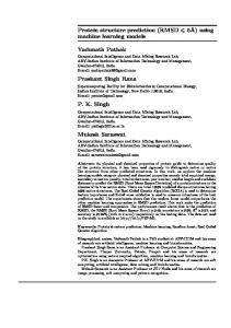
counted for more than 25%; 1% of the machines had more than two CPUs (four and eight CPUs) and provided about 5% of the computing time. Figure 6 shows that Windows OS machines (more than 87%) predominated over Linux OS machines (about 11%) and Darwin OS for Macintosh PCs (about 2%). The related total compute times showed similar values. Figure 7 shows the total number of MFold samples per target, where the numbers of amino acids for each target is reported in parenthesis. The red line in Figure 7 represents
97,108,218 230,274,379
244
3,429,779,088 4,761
8,597 8,234,990,334
number of machines Intel
compute time AMD
Macintosh
Unknown/Others
Figure 4. Number of machines and total compute time in seconds for different CPU vendors.
35,000 30,000
number of samples
590,077,072
148 2,065 3,083,553,951
8,318,520,996 11,523
number of machines
25,000 20,000 15,000 10,000 5,000 3,000
compute time n_cpu = 2
t0196 (116) t0197 (179) t0198 (235) t0199 (338) t0200 (255) t0201 ( 94) t0202 (249) t0203 (382) t0204 (351) t0205 (130) t0206 (220) t0208 (357) t0209 (239) t0210 (160) t0211 (144) t0212 (126) t0213 (103) t0214 (110) t0215 ( 76) t0216 (435) t0217 (261) t0218 (303) t0219 (330) t0221 ( 85) t0222 (373) t0223 (206) t0224 ( 87) t0228 (430) t0230 (104) t0232 (236) t0233 (362) t0234 (165) t0235 (499) t0237 (445) t0238 (244) t0239 ( 98) t0241 (237) t0243 ( 93) t0244 (301) t0247 (364) t0250 (234) t0251 (102) t0253 (194) t0254 (107) t0267 (159) t0268 (285) t0269 (250) t0270 (249) t0271 (161) t0272 (211) t0274 (159) t0275 (137) t0276 (184) t0277 (119) t0279 (261) t0280 (208) t0281 ( 70) t0282 (332)
0
n_cpu = 1
n_cpu > 2
targets
Figure 5. Number of machines and total compute time in seconds for different numbers of CPUs per PC.
245
Figure 7. Number of samples per target computed during CASP6.
230,274,379 1,166,359,365
1,552
11,914
10,595,518,275
number of machines Windows
the limit of 3,000 samples per target. For 81% of the targets we were able to run more than 3,000 samples, and for 48% we were able to overcome the 10,000 samples limit. For some targets (i.e., t0196, t0222, t0223, t0224, t0239, t0241, t0253 and t0254) we were forced to suspend the sampling before reaching the 3,000 samples because of constraints associated with the prediction submission deadlines. The current scheduling policy of BOINC does not allow us to prioritize any target over the others once their tasks have been generated and submitted. The submission of a large number of tasks whose average compute time is several hours (as it is the case for P@H) required the system to wait up to one day to get back results from the participants’ machines. The validation of results based on comparison of replicated tasks, adopted for security reasons, further increases the waiting time for final results. An extensive sampling for a given target required up to three/four days if not longer. In an attempt to keep the total time for an extensive sampling of a given target under control, we strongly decoupled the MC simulations and for each target we configured its tasks in terms of MC moves so that their length on the same type of machine needed approximately the same amount of time. For example, on an Intel single processor 1.6GHz machine running Windows OS, the compute time for a task lasted in average about 3 hours if no suspension of the computation was required or the computing resources were not heavily used by the user. On the other hand, the large number of hosts available allowed us to distribute in parallel thousands of independent tasks among participants’ machines. We did not relate the number of samples to the complexity and size of the targets but for each target we
compute time Linux
Darwin
Figure 6. Number of machines and total compute time in seconds for different OSs.
of the PCs participating in P@H deployed Intel technology and provided more than 67% of the total compute time, about 35% were based on AMD technology and supplied about 28% of the total compute time, and only a small percentage, less than 2%, used Macintosh (PowerPC) technology; the percentage of compute time provided by these machines was in the same range. The fourth class of vendors (Unknown/Others) comprised Sun machines which were not supported by P@H but tried to join the project during CASP6 and machines whose users decided not to provide the P@H server with the information related to the kind of technology they provided to the project. Such machines are classified by BOINC as unknown and their computation cannot be used by P@H because it requires a clear identification of the deployed technology for HR. In Figure 5 we can see that the compute time showed a certain tendency to scale linearly with the number of processors: 15% of the machines were dual-processors and their compute time 5
mation available. The ”Easy” category (E) contains all targets that are based on alignment with a related structure that has previously been solved as a template. Because of this wealth of information, these targets require the least amount of conformational sampling. ”Medium” targets (M) are loosely templated on an unrelated protein that may have similar structural characteristics. Targets with no template information rely solely on secondary structure prediction thus require the most sampling. Proteins of this type consisting of a single domain and a chain length under 300 residues are feasible to this approach and are considered ”Hard” (H), and those with lengths greater than 300 or those composed of multiple domains are considered ”Very Hard” (VH). The values in Table 1 underline how public-resource computing is able to advance our capability to accurately predict protein structure from sequence for reasonable targets that require extensive conformational sampling (in particular medium and hard targets).
tried to achieve as many samples as possible before the submission deadline was reached. Finally, for the largest targets with more than 440 amino acids, e.g., t0216, t0235, and t0237, MFold program limitations inhibited prediction calculations. The refinement of the sampled structures through MD simulations using the CHARMM code consisted of short independent tasks starting from the sampled conformations: on average the completion time for a task was much shorter than one hour. For example for fast machines such as an AMD Athlon 64 FX-51 processor, it ranged in average between 10 and 20 minutes. We observed that such short tasks affected the BOINC client and the network, as well as our server, with significant loads. The infrastructure limits forced us to move in several occasions the refinement computation to a cluster. From our experiments to date we learned that in general longer computational tasks are better suited for public-resource computing on the Internet, in excess of several hours preferably. However, longer tasks require the use of checkpointing techniques to allow the volunteer to “turn-off” their computer without wasting computation time and without having to reinitiate the entire calculation each time the computer is restarted. Moreover, checkpointing capability also allows participants to share their computing power among several projects powered by BOINC (i.e., P@H, SETI, climatepredictor). Therefore checkpoints have been introduced in both CHARMM and MFold.
3.2 P@H versus Cluster of PCs The benefit of the large amount of conformational sampling made available by a distributed network of public-resources was evaluated by comparison of best structures generated by P@H against results computed on a local cluster. The local cluster consisted of 64 computing nodes, each with dual 2.4 GHz Pentium Xeon processors and 1Gb of RAM, running RedHat 8.0 and interconnected with an 1 Gb Ethernet switch. Table 1 shows the accuracy of the best stuctures generated by P@H and by the local cluster calculated by comparison with the released CASP experimental structures. Available nodes on the cluster were used to run the same protein structure prediction protocol, generating 1001000 unique results for each target. The number of unique results (samples) using P@H are shown in the table for each target together with its number of amino acids (length). Some P@H targets in Figure 7 were later canceled by the CASP assessors because the experimentalists did not submit a structure before the deadline for assessment and therefore are not reported in the table. The measure used to calculate the accuracy of results is the GDT TS (Global Distance Test) score, defined as an average of the percent of residues under distance cutoffs of 1, 2, 4, and 8 Angstroms. As an average of percentages, GDT values range from 0 to 100, 0 corresponding to a poor prediction and 100 corresponding to a near-perfect prediction. The targets have been classified into 4 classes (type) based on their chain length and amount of restraint infor-
Figure 8. Comparison of final CASP protein structures obtained in laboratory with the structures obtained using the public-resources of P@H and a cluster.
6
target 196 197 198 199 200 201 202 203 204 205 206 208 209 211 212 213 214 215 216(a ) 222 223 224 228 230 a
type E H H VH M H VH M VH M VH M VH E H H H H VH M M H VH M
length 116 179 235 338 255 94 249 382 351 130 220 357 239 144 126 103 110 53 435 373 206 87 429 104
samples 2224 6463 12384 10405 10511 10629 10656 8646 8613 8607 12903 11006 11181 30690 15359 3807 3857 3878 1074 1349 1461 1314 10546 10621
P@H GDT 75.28 15.66 21.11 9.06 28.14 43.88 10.84 18.22 45.45 53.16 16.30 33.36 13.84 28.13 16.94 25.49 25.45 45.75 – 9.08 12.14 28.16 7.82 32.84
local GDT 70.22 17.77 17.50 8.12 28.03 27.13 9.34 17.40 44.78 48.54 15.94 31.47 10.35 37.68 16.94 20.63 25.68 42.92 – 8.73 12.14 28.16 7.52 27.94
target 232 233 234 235 238 239 241 243 244 247 267 268 269 271 272 274 275 276 277 279 280 281 282
type M E M M VH H M H M E M M M E H M M M E M H H M
length 236 362 165 499 244 98 237 93 301 364 175 285 250 161 211 159 137 184 119 261 208 70 332
samples 10551 7817 10182 1086 3810 1295 1162 5448 5858 7886 13160 13143 12176 11795 11758 11747 11740 11725 7562 7615 7548 7679 7572
P@H GDT 47.13 68.90 50.00 32.90 23.34 28.82 10.02 31.25 42.65 51.39 58.62 61.57 50.10 57.14 17.82 71.63 52.41 69.49 80.34 44.78 15.02 46.79 58.98
local GDT 45.00 71.16 48.70 32.90 23.34 28.82 8.97 26.70 42.40 46.88 55.13 51.33 44.42 59.78 11.57 67.31 49.63 65.63 76.71 44.09 15.02 27.86 57.59
too large for analysis, nonglobular structure
Table 1. Accuracy of the best structures generated by P@H (P@H GDT) and by a local cluster (local GDT) calculated by comparison with the released experimental structures. Low GDT values correspond to poor predictions while high values of GDT indicate good prediction. For each protein, the best GDT is reported in bold.
A representative example for each type of protein is shown in Figure 8. The top structures are the results from publicresource computing, local cluster computing, and experimental results for target t0271. Because it is an ”easy” target based on a good template, it does not require extensive sampling, and there is no improvement for the P@H structure (GDT 57.14) over the local cluster structure (GDT). T0205 is a ”medium” difficulty target with a significant improvement from P@H sampling (GDT 53.16) over local sampling (GDT 48.54). Target t0198 similarly benefits from increased sampling as a ”hard” target (GDT 21.11 vs 17.50). However, ”very hard” targets such as t0199 often do not get significantly better structures from P@H over local clusters (GDT 9.06 and 8.12, respectively) due to both extremely large conformational space and the limited ability of the sampling algorithm to deal with multi-domain proteins.
variety of heterogeneous machines with different compute speeds, architectures and operating systems interconnected to the Internet. Nevertheless we were able to guarantee the integrity and security of the returned data in an efficient way by deploying homogeneous redundancy and strict equality to compare the redundant results. From our observations we conclude that the benefit of a large amount of conformational sampling is visible for homology modeling targets, and especially for fold recognition targets as well as small targets with a complete absence of templated regions. For ”new fold” targets with more than 300 residues and composed of more than one domain, the extensive sampling afforded by P@H does not yield satisfactory results suggesting a limitation in accuracy of the protocol deployed. Our final goal behind the effort presented in this paper is to establish, by utilizing the vast supercomputer that is the Internet, a truly significant tool for automated structure prediction avaliable to a broad audience and accessible through a web portal for a wider range of applications such as ligand docking, loop modeling, etc.
4 Discussion and Future Work The key objective of the presented research has been to evaluate the potential of utilizing the P@H/BOINC system for testing of structure prediction algorithms based on conformational sampling. Over the duration of CASP6, P@H has benefited from more than 12 billion seconds for sampling conformations of protein structures. The computing power was supplied by a
Acknowledgments Financial support from the National Institutes of Health Grant, RR12255 is greatly appreciated. Financial support through the NSF sponsored Center for Theoretical Biological Physics (grants# PHY-0216576 and 0225630) and the LJIS Fund are acknowledged.
7
We wish to thank David Anderson and Rom Walton for their invaluable help with Predictor@Home and the Predictor@Home and BOINC community of volunteers for donating their computing cycles.
[16] ClimaterPrediction.net: a Forecast of the Climate in the 21st Century. http://climateprediction.net, 2004. [17] A. Olson and et Al. FightAIDS@Home: Accelerate AIDS Research by Deploying Global ”Grid” of Distributed Computing Power. http://fightaidsathome.scripps.edu. [18] The United Devices Cancer Research Project. http://www.grid.org, 2002. [19] V. Pande and et Al. Atomistic Protein Folding Simulations on the Submillisecond Time Scale Using Worldwide Distributed Computing. Biopolymers, 68:91–109, 2003. [20] M. Shirts and V. Pande. Screen Savers of the World, Unite! Science, 2000. [21] S.F. Altschul, T.L. Madden, A.A. Schffer, J. Zhang, Z. Zhang, W. Miller, and D.J. Lipman. Gapped BLAST and PSI-BLAST: a New Generation of Protein Database Search Programs. Nucleic Acids Res, 25:3389–3402, 1997. [22] K. Karplus, R. Karchin, J. Draper, J. Casper, Y. MandelGutfreund, M. Diekhans, and R. Hughey. Combining LocalStructure, Fold-Recognition and New-Fold Methods for Protein Structure Prediction. Proteins, 53:491–496, 2003. [23] L.J. McGuffin, K. Bryson, and D.T. Jones. The PSIPRED Protein Structure Prediction Server. Bioinformatics, 16:404– 405, 2000. [24] J. Skolnick, A. Kolinski, and A.R. Ortiz. MONSSTER: A Method for Folding Globular Proteins with a Small Number of Distance Restraints. J Mol Biol, 265:217–241, 1997. [25] B.R. Brooks, R.E. Bruccoleri, B.D. Olafson, D.J. States, S. Swaminathan, and M. Karplus. CHARMM: A Program for Macromolecular Energy Minimization, and Dynamics Calculations. J Comp Chem, 4:187–217, 1983. [26] A.D. MacKerell Jr., B. Brooks, C.L. Brooks III, L. Nilsson, B. Roux, Y. Won, and M. Karplus. CHARMM: The Energy Function and Its Parameterization with an Overview of the Program. The Encyclopedia of Computational Chemistry, 1:271–277, 1998. P. v. R. Schleyer et al., editors (John Wiley and Sons: Chichester). [27] M.S. Lee, M. Feig, F.R. Salsbury Jr., and C.L. Brooks III. New Analytic Approximation to the Standard Molecular Volume Definition and its Application to Generalized Born Calculations. J Comput Chem, 24:1348–1356, 2003. [28] M. Feig, J. Karanicolas, and C.L. Brooks III. MMTSB Tool Set: Enhanced Sampling and Multiscale Modeling Methods for Applications in Structural Biology. J of Molecular Graphics and Modeling, 22:377–95, 2004. [29] D.P. Anderson and J. Kubiatowicz. The World-Wide Computer. Scientific American, March 2002. [30] D.P. Anderson. BOINC: A System for Public-Resource Computing and Storage. In Proceedings of the 5th IEEE/ACM International Workshop on Grid Computing, Pittsburgh, PA, November 2004. [31] M. Taufer, D.P. Anderson, P. Cicotti, and C.L. Brooks III. Homogeneous Redundancy: a Technique to Ensure Integrity of Molecular Simulation Results Using Public Computing. Denver, Colorado, April 2005. Proceedings of the 14th Heterogeneous Computing Workshop HCW (2005), in conjunction with IPDPS 2005. [32] M. Braxenthaler, R. Ron Unger, D. Auerbach, J.A. Given, and J. Moult. Chaos in Protein Dynamics. Proteins, 29(417– 425), 1997.
References [1] B. Rost. Marrying Structure and Genomics. 6:256–263, 1998.
Structure,
[2] H.M. Berman, J. Westbrook, Z. Feng, G. Gilliland, T.N. Bhat, H. Weissig, I.N. Shindyalov, and P.E. Bourne. The Protein Data Bank. Nucleic Acids Research, 28:235–242, 2000. [3] E. Gasteiger, A. Gattiker, C. Hoogland, I. Ivanyi, R.D. Appel, and A. Bairoch. ExPASy: the Proteomics Server for InDepth Protein Knowledge and Analysis. Nucleic Acids Res., 31:3784–3788, 2003. [4] K.C. Worley, P Culpepper, B.A. Wiese, and R.F. Smith. BEAUTY-X: Enhanced BLAST Searches for DNA Queries. Bioinformatics, 14(10):890–1, 1998. [5] A. Marchler-Bauer, A.R. Panchenko, B.A. Shoemaker, P.A. Thiessen, L.Y. Geer, and S.H. Bryant. CDD: a Database of Conserved Domain Alignments with Links to Domain Three-Dimensional Structure. Nucleic Acids Res, 30:281– 283, 2002. [6] Y. Wang, J.B. Anderson, J. Chen, L.Y. Geer, S. He, D.I. Hurwitz, C.A. Liebert, T. Madej, G.H. Marchler, A. MarchlerBauer, A.R. Panchenko, B.A. Shoemaker, J.S. Song, P.A. Thiessen, R.A. Yamashita, and S.H. Bryant. MMDB: Entrez’s 3D-Structure Database. Nucleic Acids Res, 30:249– 252, 2002. [7] J.N. Onuchic, Z. Luthey-Schulten, and P.G. Wolynes. Theory of Protein Folding: The Energy Landscape Perspective. Ann Rev Phys Chem, 48:545–600, 1997. [8] H. Frauenfelder, S. Sligar, and P.G. Wolynes. The Energy Landscapes and Motions of Proteins. Science, 254:1598– 1603, 1991. [9] P.G. Wolynes and Z. Luthey-Schulten. The Energy Landscape Theory of Protein Folding Physics of Biological Systems: From Molecules to Species. H. Flyvbjerg, J. Hertz, Mogens H. Jensen, Ole G. Mouritsen, K. Sneppen, eds. (Springer-Verlag, Berlin), pages 61–79, 1996. [10] M. Eastwood, C. Hardin, Z. Luthey-Schulten, and P.G. Wolynes. Evaluating Protein Structure Prediction Schemes Using Energy Landscape Theory. IBM J Res Development, 45:475–497, 2001. [11] J. Moult, K. Fidelis, A. Zemla, and T. Hubbard. Critical Assessment of Methods of Protein Structure Prediction (CASP)-Round V. Proteins, 53(6):334–9, 2003. [12] M. Feig and C.L. Brooks III. Evaluating CASP4 Predictions With Physical Energy Functions. Proteins, 49:232–245, 2002. [13] B.N. Dominy and C.L. Brooks III. Identifying Native-like Protein Structures using Physics-based Potentials. J Comp Chem, 23:147–160, 2001. [14] T. Lazaridis and M. Karplus. Effective Energy Function for Proteins in Solution. Proteins, 35:133–152, 1999. [15] D.P. Anderson. SETI@Home: Search for Extraterrestrial Intelligence at Home. http://setiathome.ssl.berkeley.edu.
8