Over the last few years there was an explosion of mathematical research related ...... Department of Mathematics and Statistics, Dalhousie University, Halifax NS, ...
PURSUIT-EVASION IN MODELS OF COMPLEX NETWORKS ANTHONY BONATO, PAWEÃL PRAÃLAT, AND CHANGPING WANG
Abstract. Vertex pursuit games, such as the game of Cops and Robbers, are a simplified model for network security. In these games, cops try to capture a robber loose on the vertices of the network. The minimum number of cops required to win on a graph G is the cop number of G. We present asymptotic results for the game of Cops and Robbers played in various stochastic network models, such as in G(n, p) with non-constant p, and in random power law graphs. We find bounds for the cop number of G(n, p) for a large range of p as a function of n. We prove that the cop number of random power law graphs with n vertices is asymptotically almost surely Θ(n). The cop number of the core of random power law graphs is investigated, and is proved to be of smaller order than the order of the core.
1. Introduction Suppose that an intruder is loose on the vertices of a network, and travels between adjacent vertices. The intruder could represent a virus or hacker, or some other malicious agent intent on avoiding capture. A set of searchers are attempting to capture the intruder. Although placing a searcher on each vertex guarantees the capture of the intruder, it is a more interesting (and more difficult) problem to find the minimum number of searchers required to capture the intruder. A motivation for minimizing the number of searcher comes from the fact that fewer searchers require fewer resources. Networks that require a smaller number of searchers may be viewed as more secure than those where many searchers are needed. Vertex pursuit games, such as Cops and Robbers, may be viewed of as a simplified model for such network security problems. The game of Cops and Robbers, introduced independently by Nowakowski and Winkler [16] and Quilliot [17] over twenty years ago, is played on a fixed graph G, and is our focus in this study. We will always assume that G is undirected, simple, and finite. There are two players, a set of k cops (or searchers), where k > 0 is a fixed integer, and the robber. The cops begin the game by occupying a set of k vertices. The robber then chooses a vertex, and the cops and robber move in alternate rounds. The players use edges to move from vertex to vertex. More than one cop is allowed to occupy a vertex, and the players may remain on their current vertex. The players know each others current locations and can remember all the previous moves. The cops win and the game ends if at least one of the cops can eventually occupy the same vertex as the robber; otherwise, the robber wins. As placing a cop 1991 Mathematics Subject Classification. 05C80, 68R10, 94C15. Key words and phrases. random graphs, complex networks, vertex-pursuit games, Cops and Robbers, domination, adjacency property. The authors gratefully acknowledge support from NSERC and MITACS. 1
2
ANTHONY BONATO, PAWEÃL PRAÃLAT, AND CHANGPING WANG
on each vertex guarantees that the cops win, we may define the cop number, written c(G), which is the minimum number of cops needed to win on G. The cop number was introduced by Aigner and Fromme [1] who proved (among other things) that if G is planar, then c(G) ≤ 3. For a survey of results on vertex pursuit games such as Cops and Robbers, the reader is directed to the surveys [2, 11, 12]. Over the last few years there was an explosion of mathematical research related to stochastic models of real-world networks, especially for models of the web graph. Many technological, social, biological networks have properties similar to those present in the web, such as power law degree distributions and the small world property. Following [9], we refer to these networks as complex. For example, power laws have been observed in protein-protein interaction networks, and social networks such as the one formed by scientific collaborators. While much of the earlier mathematical work on complex networks focused on designing models satisfying certain properties such as power law degree distributions, new approaches are constantly emerging. For additional background on complex networks and their models, see [3, 9]. In this paper, which is the full version of [7], we study vertex pursuit games in random graph models, including models for complex networks. While Cops and Robbers have been extensively studied in highly structured deterministic graphs such as graph products (see [15]), our work is the first to consider such games in models of complex networks. All asymptotics throughout are as n → ∞. We say that an event in a probability space holds asymptotically almost surely (a.a.s.) if the probability that it holds tends to 1 as n goes to infinity. For p ∈ (0, 1) or p = p(n) tending to 0 with n, define Ln = log 1 n. We denote the incomplete gamma function by Γ(·, ·). 1−p We consider Erd˝os, R´enyi G(n, p) random graphs and their generalizations used to model complex networks. The random graph G(n, p) consists of the probability space (Ω, F, P), where Ω is the set of all graphs with vertex set [n] = {1, 2, . . . , n}, F is the family of all subsets of Ω, and for every G ∈ Ω n P(G) = p|E(G)| (1 − p)( 2 )−|E(G)| . ¡ ¢ This space may be viewed as n2 independent coin flips, one for each pair of vertices, where the probability of success (that is, drawing an edge) is equal to p. Note that p = p(n) can tend to zero with n. The cop number of G(n, p) was studied in [6], where the following result was proved.
Theorem 1.1. Let 0 < p < 1 be fixed. For every real ε > 0 a.a.s. for G ∈ G(n, p) (1 − ε)Ln ≤ c(G) ≤ (1 + ε)Ln. The problem of determining the cop number of G(n, p) where p = p(n) is a function of n was left open in [6]. In [5] it was shown that the cop number of G(n, p) is always bounded from above by n1/2+o(1) and this bound is achieved for sparse random graphs. √ More precisely, they showed that c(G(n, p)) ≤ 160000 n log n for np ≥ 2.1 log n and c(G(n, p)) ≥
1 log log(np)−9 1 2 log log(np) n (np)2
PURSUIT-EVASION IN MODELS OF COMPLEX NETWORKS
3
for np → ∞. Since if either np = no(1) or np = n1/2+o(1) , then a.a.s. c(G(n, p))√= n1/2+o(1) , it would be natural to assume that the cop number of G(n, p) is close to n also for np = nα+o(1) , where 0 < α < 1. In [14] it was shown that the actual behaviour of c(G(n, p)) is more complicated. Function f : (0, 1) → R defined as f (x) =
log E(c(G(n, nx−1 ))) , log n
where E(c(G(n, p))) denotes the expected value of the cop number for G(n, p). The main result of [14] was that f has an unexpected zigzag shape; see Figure 1.
Figure 1. The ‘zigzag’ function f . In the next subsection, we show that if np = nα+o(1) , where 1/2 < α ≤ 1, then a.a.s. c(G(n, p)) = Θ(log n/p) = n1−α+o(1) and c(G(n, n−1/2+o(1) )) = n1/2+o(1) a.a.s. This result is used in [14] where the main focus is on 0 < α < 1/2. Recent work of Chung and Lu [8, 9] supplies an extension of the G(n, p) random graphs to random graphs G(w) with given expected degree sequence w. For example, if w follows a power law distribution, then G(w) supplies a model for complex networks. We determine bounds on the cop number of random power law graphs as discussed in the next subsection. 1.1. Results. We consider the cop number in classical random graphs and for random power law graphs. The proofs of the results in this subsection may be found in Section 2. We consider the cop number of G(n, p(n)) when p(n) is a function of n. We will abuse notation and refer to p rather than p(n). For G(n, p) our main results are summarized in the following theorem. Theorem 1.2. (1) Suppose that p ≥ p0 where p0 is the smallest p for which ¡ ¢ log (log2 n)/p 2 p /40 ≥ log n
4
ANTHONY BONATO, PAWEÃL PRAÃLAT, AND CHANGPING WANG
holds. Then a.a.s. G ∈ G(n, p) satisfies ¡ ¢ ¡ ¢ Ln − L (p−1 Ln)(log n) ≤ c(G) ≤ Ln − L (Ln)(log n) + 2. √ (2) If (2 log n)/ n ≤ p = o(1) and ω(n) is any function tending to infinity, then a.a.s. G ∈ G(n, p) satisfies ¡ ¢ Ln − L (p−1 Ln)(log n) ≤ c(G) ≤ Ln + L(ω(n)). The proof may be found in Subsection 2.1 below. By Theorem 1.2, we have the following corollary. Corollary 1.3. If p = n−o(1) and p < 1, then a.a.s. G ∈ G(n, p) satisfies c(G) = (1 + o(1))Ln. Indeed, from part (1) it follows that if p is a constant, then c(G) = Ln − 2L log n + Θ(1) = (1 + o(1))Ln. From part (2), for p = n−o(1) tending to zero with n, the lower bound is ¡ ¢ ¡ ¢ Ln − L (p−1 Ln)(log n) = Ln − 2L (1 + o(1))p−1 log n ¡ ¢ = Ln − 2L no(1) = (1 + o(1))Ln. Note also that for p = n−a(1+o(1)) (0 < a < 1/2) we do not have a concentration for c(G) but the following bounds hold (1 + o(1))(1 − 2a)Ln ≤ c(G) ≤ (1 + o(1))Ln. We now describe results for the cop number of random power law graphs. Let w = (w1 , . . . , wn ) be a sequence of n nonnegative real numbers. We define a random graph model, written G(w), as follows. Typically, vertices are integers in [n]. Each potential edge between i and j is chosen independently with probability pij = wi wj ρ, where 1 ρ = Pn i=1
wi
.
We will always assume that max wi2 < i
n X
wi ,
i=1
which implies that pij ∈ [0, 1). The model G(w) is referred to as random graphs with given expected degree sequence w. Observe that G(n, p) may be viewed as a special case of G(w) by taking w to be equal the constant n-sequence √ (pn, pn, . . . , pn). Given β > 2, d > 0, and a function M = M (n) = o( n) (with M tending to infinity with n), we consider the random graph with given expected degrees wi > 0, where 1
wi = ci− β−1
(1)
PURSUIT-EVASION IN MODELS OF COMPLEX NETWORKS
5
for i satisfying i0 ≤ i < n + i0 . The term c depends on β and d, and i0 depends also on M ; namely, ¶ ¶¶β−1 µ µ µ 1 β−2 β − 2 d c= dn β−1 , i0 = n . (2) β−1 M β−1 It is not hard to show (see [8, 9]) that a.a.s. the random graphs with the expected degrees satisfying (1) and (2) follow a power law degree distribution with exponent β, average degree (1 + o(1))d, and maximum degree (1 + o(1))M . Our next theorem demonstrates that the cop number of random power law graphs is a.a.s. Θ(n), and so is of much larger order than the logarithmic cop number of G(n, p) random graphs. Hence, these results are suggestive that in power law graphs, on average a large number of cops are needed to secure the network. Theorem 1.4. For a random power law graph G ∈ G(w) with exponent β > 2 and average degree d, a.a.s. the following hold. (1) If X is the random variable denoting the number of isolated vertices in G(w), then c(G) ≥ X
µ
¶ β − 2 −1/(β−1) exp −d = (1 + o(1))n x dx β−1 0 ¶ µ β−2 β−1 2−β . = (1 + o(1))(d(β − 2)) (β − 1) nΓ 1 − β, d β−1 Z
(2) For a ∈ (0, 1), define Z f (a) = a +
1 a
1
µ
¶ β − 2 (β−2)/(β−1) −1/(β−1) exp −d a x dx. β−1
Then c(G) ≤ (1 + o(1))n min f (a). 0 (2 log n)/ n and ¥ ¡ ¢¦ k = Ln − L (p−1 Ln)(log n) , (6) then a.a.s. G ∈ G(n, p) is (1, k)-e.c. Note that we do not use the condition for p in the proof of the theorem. The condition is introduced in order to get a non-trivial result; the value of k is negative otherwise. Proof. Assume that p = o(1). Then µ
¶ log2 n k = Ln − L (1 + o(1)) 2 p µ ¶ log n = Ln − 2L (1 + o(1)) . p Fix S a k-subset of vertices and a vertex u not in S. For a vertex x ∈ V (G)\(S ∪{u}), the probability that a vertex x is joined to u and to no vertex of S is p(1 − p)k . Since edges are chosen independently, the probability that no suitable vertex can be found for this particular S and u is (1 − p(1 − p)k )n−k−1 . Let X be the random variable counting the number of S and u for which no suitable x can be found. We then have that µ ¶ ¡ ¢n−k−1 n (n − k) 1 − p(1 − p)k E(X) = k µ ¶n(1−(Ln)/n) (Ln)(log n) k+1 ≤ n 1− n = nk+1 exp (−(Ln)(log n)(1 − (Ln)/n)) (1 + o(1)) ¡ ¢ = nk+1 exp −(Ln − (Ln)2 /n)(log n)(1 + o(1)) ¶ µ ³ 2 log log n 2 log2 n ´ k+1 − (log n)(1 + o(1)) ≤ n exp − k + p p2 n µ ³ ¶ 2 log log n ´ k+1 = n exp − k + (log n)(1 + o(1)) p = o(1), where the second inequality follows by (5). It is also easy to show that the same argument holds for p a constant. The proof now follows by Markov’s inequality. ¤
PURSUIT-EVASION IN MODELS OF COMPLEX NETWORKS
9
2.2. Extreme cases. It is known that if p is tending to one pretty fast, then the maximum degree of a random graph is very large. Formally, for a fixed non-negative integer k, if n(1 − p) − log n − k log log n → −∞, then the maximum degree is at least n − 1 − k a.a.s. and clearly k + 1 is an upper bound for a cop number (one cop can occupy a vertex with maximum degree). We next provide a concentration result for the cop number of the random graphs G(n, p) for p approaching zero very fast. For example, if p = o(1/n2 ), a.a.s. G ∈ G(n, p) is empty. In this range of p a.a.s. the cop number of G is n. We now consider the case when p = d/n for constant d ∈ (0, 1). Bollob´as [4] proved the following result. Theorem 2.4. Let 0 < d < 1, p = d/n, and let X be the number of tree connected components of G(n, p). Then the expectation of X is E(X) = u(d)n + O(1), where ∞
1 X k k−2 −d k u(d) = (de ) . d k=1 k! A.a.s. G(n, p) satisfies |X| = (1 + o(1))u(d)n. We note that u(d) ∈ (0, 1). A graph is unicyclic if it contains exactly one cycle. Theorem 2.5. Let 0 < d < 1 and p = d/n. Then a.a.s. G ∈ G(n, p) is such that every connected component is a tree or a unicyclic graph, and there are at most log log n vertices in the unicyclic components. Trees are cop-win graphs, while unicyclic graphs have cop number at most 2. Each tree component requires exactly one cop, while there are at most 2 log log n many cops needed for all the unicyclic components. Hence, the number of cops on the unicyclic components becomes negligible in contrast to the number of cops on tree components. Therefore, from Theorems 2.4 and 2.5 we have the following concentration result. Corollary 2.6. Let 0 < d < 1, p = d/n. Then for the graph G ∈ G(n, p), E(c(G)) = u(d)n + O(log log n). A.a.s. G ∈ G(n, p) satisfies c(G) = (1 + o(1))u(d)n. 2.3. The proof of Theorem 1.4. Proof. For the lower bound, we exploit the fact that the cop number is bounded from below by the number of isolated vertices: one cop is needed per isolated vertex. In general power law graphs, there may exist an abundance of isolated vertices, even as much as Θ(n) many. We show that this is indeed the case for random power law graphs.
10
ANTHONY BONATO, PAWEÃL PRAÃLAT, AND CHANGPING WANG
The probability that the vertex i for i0 ≤ i < n + i0 (that is, the vertex i corresponds to the weight wi ) is isolated is equal to Y pi = (1 − wi wj ρ) j,j6=i
=
Y
j,j6=i
exp (−wi wj ρ(1 + o(1))) Ã
= exp −wi ρ
X
! wj (1 + o(1))
j,j6=i
= exp (−wi (1 + o(1))) .
(7)
Let Xi be an indicator random variable for the event that the vertex i is isolated. Then P(Xi = 1) = 1 − P(Xi = 0) = pi for i0 ≤ i < n + i0 . P Let X be the number of isolated vertices in G(w). As X = i0 ≤i