Q-SAC: Toward QoS Optimized Service Automatic Composition* Hanhua Chen, Hai Jin, Xiaoming Ning, Zhipeng Lü Cluster and Grid Computing Lab Huazhong University of Science and Technology, Wuhan, 430074, China Email:
[email protected]
Abstract The emerging service grids bring together various distributed services to a ‘market’ for clients to request and enable the integration of services across distributed, heterogeneous, and dynamic virtual organizations. In the experience of constructing and using the ChinaGrid, we meet two challenges, optimizing the QoS of the grid resources and minimizing complexity for application users and developers. In this paper, we present Q-SAC, a QoS optimized service automatic composition model to address these problems. Two main features of Q-SAC are (1) automatic grid service composition, and (2) global level multidimensional QoS optimization for the composition plan. We design the algorithms for generating and optimizing the composite services. The simulation results show that our model and solution are practical and efficient.
1. Introduction The emerging grid technologies have been widely adopted in science and technical computing. It supports the sharing and coordinated use of diverse resources in dynamic, distributed virtual organizations, that is, the creation, from geographically distributed components operated by distinct organizations with different policies, of virtual computing systems that are sufficiently integrated to deliver the desired Quality of Services (QoS) [1]. Recently, the grid is evolving to the Open Grid Services Architecture (OGSA) [2], which brings together various distributed application-level services to a ‘market’ for clients to request and enable the integration of services across distributed, heterogeneous, dynamic virtual organizations.
In our early experience in developing ChinaGrid Supporting Platform (CGSP) [3], a middleware platform that addresses building a service-oriented grid based on Web Service Resource Framework (WSRF) [4], we found two major challenges. One is to make the satisfactory use of the grid resources to guarantee QoS. The other is to minimize complexity for grid users and developers; that is, grid-based applications should be user-friendly and minimal training is necessary. To address these problems, we propose Q-SAC, a QoS-Optimized Service Automatic Composition model in this paper. Two main features of Q-SAC are (1) automatic grid service composition, and (2) global level multidimensional QoS optimization for the composition plan. The rest of this paper is organized as follows. Section 2 introduces the semantic based service virtualization mechanism, which is the main assumption of Q-SAC. We describe the automatic service composition method in section 3. Section 4 establishes the mathematical model for optimizing QoS of the composite plan and proposes the algorithms for solution. Section 5 shows the simulation results of QSAC. Section 6 reviews some related works. Section 7 concludes the paper and describes our future work.
2. Semantic based Service Virtualization 2.1 Service Virtualization Service-oriented view simplifies service virtualization through encapsulation of diverse implementations behind a common service interface. [5] introduces a service grid prototype using Legion to explore the design of application and service based replica selection policies in a wide-area network. However the semantic of the service cannot be
* This paper is supported by National Science Foundation under grant 60273076 and 90412010, ChinaGrid project from Ministry of Education, and the National 973 Key Basic Research Program under grant No.2003CB317003.
0-7803-9074-1/05/$20.00 ©2005 IEEE
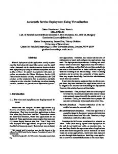
specified and the replicas of the same service are developed and deployed by the same provider. Our service virtualization model provides an extensible set of Virtual Services (VS) to users (see Figure1).
Figure 1.
Service virtualization
Each VS is defined as uniform service semantics in a specific domain. We call an implementation of VS a Physical Service (PS). Thus, each VS is implemented as a vector of redundant PSs with different QoS. From the functional aspect, each VS may include a vector of functions (operations). Thus we use the following expression to describe a VS: t
(
VS = F1 , F2 t
t
t
LF ) t
v
L O O L O M M M M O L O
PS1 O11 t t PS O = 2 = 21 PS t O t u u1
Ftk
M
th
t
t
O12
t
t
22
2v
t
Service
1:n
1:1
1:n
1:1
1:1
1:1
1v
t
u2
In Figure 2, we describe the proposed ontology using a directed graph. Here, nodes represent the concepts of ontology. Unfilled nodes refer to WSDL concepts. Gray nodes refer to extended feature introduced to augment WSDL descriptions with semantic capabilities. In our QoS-aware automatic service composition model we pay more attention to the functionality semantic and QoS semantic of grid service operations. The node Function Rule accurately describes the function of the service in a specific domain. Each operation has one Function Rule [7], which expresses that the service is capable of producing particular outputs of the given certain inputs. The function rules are registered in a rule repository when grid services are published. We believe that as the number of grid services that offer overlapping or similar functionality increases, QoS will be one of the substantial aspects for differentiating between similar service providers. The QoS metrics used to define QoS capabilities have to be ontologically defined because they can be very easily misinterpreted [8]. Q-SAC gives accurate definition of five kinds of application level QoS metrics, including price, execution time, reputation, availability, and successful rate.
(1)
t
uv
th
denotes the k function of the t virtual where service and PStk denotes the kth physical service of the tth virtual service. Otij denotes the jth operation of tth virtual service provided by ith service provider. We use Qtij to describe the QoS information of Otij: Qtij = Quality(Otij) (2) and thus the QoS information of tth VS can be described as the following matrix: Qvst=( Qtij; 1≤i≤u,1≤j≤v) (3)
2.2 Service semantic The semantic of grid services is crucial to enabling automatic composition. To help understand semantic features of grid services, we use the concept of ontology. Ontology is a shared conceptualization based on the semantic proximity of terms in a specific domain and is expected to play a central role in the semantic web service composition [6].
Name
1:1
Binding
1: (0,1)
Name
Operation
1: (0,1)
Input
Output 1:n
1:1
Quality
Secuturity
1:n 1:1 Price
1:1
1:1 Type
Figure 2.
Provider
Domain
1:1
1:1 Function Rule
Parameter
Name
Purpose
1:1 Execution Time
1:1
1:1
1:1
Reputation
Availability
Successful rate
1:1 Unit
Ontology description of grid services
3. Service Composition When a developer wants to create a new composite service, he specifies the inputs and anticipant outputs of the composite service and submits it to Q-SAC. QSAC uses the rule engine to determine whether the service composition can be successful. In this section, we present the algorithm for generating the composition service. The algorithm is trying to deduce the output from input with the rule repository and it forms the core of the rule engine.
Figure 3.
Selecting rules in the rule repository
R ⇐ R − rj ; Ru ⇐ Ru U rj ;
each customer, the customer ID is inputted to Q-SAC and the output of mail service type with the price is expected. Figure 3 shows the rule repository and the selected rules by the generation algorithm. In Figure 4 we get a composition path. The algorithm selects necessary rules from the rule repository for generating the composition path. The implementation should be based on an accessorial rulebased expert system. We specify a composition service in the form of a directed acyclic graph on the assumption that cyclic structure can be transformed into acyclic structure.
U A)
4.QoS-optimized Grid Service Composition
We define the input set of the user as X, and the output of the user as Y, the rule set in the rule repository as R. Ru denotes the rules that have been selected in the process of deducing the output. Ru is recorded for generating the execution path. The algorithm is described as below: (1) X (0) = X , Ru = Φ, A = Φ; (2)
(
ALL Yj ⊆ X
FOR
{ ((
IF Yj
( (
j
IF Y ⊆ X
(
(3) IF X
X
)
)
(
→Z j ∧ ( rj ∈ ( R − Ru ) ) ∧ ∃( z ∈ Z j ) z ∉ X (i) rj
{A ⇐ A U Z ; (i +1)
( i +1)
(i )
(i )
⇐X
=X
( i)
(i)
{}
)
GOTO ( 5) ;
}
U A;
GOTO ( 3) ;
}
) {X
+
=X
( i +1)
{}
))
}
; GOTO ( 4) ;
ELSE GOTO ( 2 ) ;
(4) IF (Y ⊄ X + ) REPORT " No AVAILABLE EXCUTION PATH "; ELSE
(5)
GOTO ( 5 ) ;
GENERATE PATH WITH
Figure
4.
Ru ;
Generated composition path
We give the following example for the algorithm. In this scenario, a plaza plans to give birthday gifts to the registered customers for the anniversary celebration. The type of gifts depends on hobbies and ranks of the customers. Now the manager wants to make sure how much budget will be planned for sending the gifts. For
In the composition path, for each atomic operation, there may be different candidate providers with different QoS. In this section, we first present the quality metrics in the context of elementary physical service operation and then establish the QoS optimizing model for composite services.
4.1 QoS of grid services We consider five generic quality metrics for each elementary operation: execution duration, reputation, successful execution rate, availability, and price. The quality of a given operation Qtij can be defined as a vector: Qtij=(Qtij.duration, Qtij.reputation, Qtij.suc_rate, Qtij.availability, Qtij.price ) (4) (1)Execution duration Given an operation Otij, the execution duration measures the expected delay between the moment when a request is sent and the moment when the results are received. In our previous work [9], the execution duration is made up of three parts including computing time Tcom(Otij), middleware time Tmid(Otij), and
transmission time Tnet(Otij). The execution duration is quantified as below: Qtij.duration = Tcom(Otij)+ Tmid(Otij)+ Tnet(Otij) (5) Tcom(Otij) refers to the processing time of the operation. If the bandwidth and latency are fixed, Tnet(Otij) can be defined below:
( )
Tnet Oij = t
data _ sizeinput + data _ sizeoutput bandwidth
+ latency
(6)
The middleware time cost is based on existing middleware. We simply specify the upper limit of the overall middleware cost Tmid(Otij). Although we have described how to guarantee the network bandwidth between two grid nodes and how to guarantee and specify the metrics of Tcom(Otij) and Tmid(Otij) in [9], Tnet(Otij) is difficult to specify as the data size of services varies momentarily and the network latency is difficult to guarantee. Here, in order to facilitate resolving the model, we assume the invariability of data_sizeinput+data_sizeoutput and specify the network latency as a statistical feedback. (2) Reputation Qtij.reputation is a measure of the trustworthiness of t O ij [11]. The value of the reputation is defined as average ranking given to Otij by end users: Qij .reputaion = t
∑
w k =1
( ) t ij
Rk O
(7)
( ) (O )
N success Oij N total
Qij .availability =
(8)
t ij
( ) t ij
MTTF O
( ) + MTTF (O ) t ij
MTTR O
t ij
(9)
where MTTF(Otij) is the Mean Time to Failure for Otij and MTTR(Otij) is the Mean Time to Repair for Otij. (5) Price Qtij.proce is defined as the price charged for Otij by the provider.
4.2 Multi-dimension QoS scale
max (Q tjk ) − Q ijkt max ( Q tjk ) − min ( Q tjk ) 1
Q − min (Q ) ( ) = max (Q ) − min (Q ) t ijk
w
(4) Availability Qtij.avalability is the probability that Otij is accessible. It is defined as: t
t
t
t
t
( )
V Qijk =
V Q ijk
where Rk(Otij) is the kth end user’s ranking on the reputation of Otij and w is the number of times the service has been graded. (3) Successful execution rate As defined in our previous work [10], Qtij.suc_rate is defined as the times of successful Otij invocations in proportion to the total times of Otij invocations: Qij .suc _ rate =
We assign a number to each dimension of the vector, from 1 to 5. The numbers denote duration, reputation, successful rate, availability, and price in tern. Thus Qvst can be described as a three-dimension matrix: Qvst=( Qtijk; 1≤i≤u,1≤j≤v, 1≤k≤5) (10) According to method proposed in [11], we classify the quality metrics into three types. The first type, including Qtij.duration, is negative, i.e. the higher the value, the lower the quality. Another type is positive metrics, including Qtij.reputation, Qtij.suc_rate, Qtij.availability, i.e. the higher the value, the higher the quality. Particularly we classify Qtij.price into a separate type. The method proposed in [11] is adopted to eliminate the contrary characteristics between negative metrics and positive metrics. For negative metrics, values are scaled according to (11). For positive metrics, values are scaled according to (12). Particularly, we scale the value of price according to (13). Here, i denotes the sequence number of the candidate operation providers.
t jk
t jk
t jk
1
( ) t
( if max ( Q if max ( Q if max ( Q
) ( ) − min (Q ) − min (Q ) − min (Q
) ) =0 ) ≠0 ) =0
if max Qjk − min Qjk ≠ 0 t
t jk t jk t jk
t
t jk t jk t jk
t
V Qij 5 = Qij . price
(11)
(12) (13)
Based on the expression of V(Qtijk), formula (14) is used to describe the max performance/price for the jth function of the tth VS. The weight vector ω=(ωk; 1≤k≤5, ∑ωk=1) is provided by the user, where value of ωk expresses how much attention should be paid for the kth quality metric. t t max ( Qtj1 ) − Qijt 1 Qijk − min ( Q jk ) 4 * ω1 + ∑ k = 2 ∗ ωk (14) t t t t max Q min Q max Q min Q − − ( j1 ) ( j1 ) ( jk ) ( jk ) V Qtj = Max t Qij 5 * ω5
( )
The QoS metrics of our model include but are not limited to the five ones. New metrics can be flexibly added with the model unchanged. 4.3 QoS-optimized service composition model Based on the above description, we establish the mathematical model for optimizing the composition plan. The main idea of the model is to optimize performance/price of the composition plan under the precondition that the total duration and total price of the composition plan are guaranteed within the limit given by the user. The mathematical model is described as below:
Given condition (1)~(4) (1) The directed acyclic graph G(E, V) for the execution path has been generated. Here V stands for the operation set V={O1, O2, …, On} involved in the execution path and E is the set of the directed edges, which denote the relation among the operations; (2) ∀ (VS t ) ∈ Grid , the quality matrix Qvst=( Qtijk;
1≤i≤u,1≤j≤v, 1≤k≤5) is known; (3) The user gives the duration limit of the composition service as Ttotal, and the price limit of the composition service as Ptotal; (4) The user gives the weight vector ω=(ωk; 1≤k≤5, ∑ωk=1). Objective function and constraints We want to find a solution, a composition plan X=(x1, x2, …, xn), where xi is selected from all candidate providers, with the optimized QoS expressed as the objective function (15) and two constraints (16) and (17). Here, in objective function (16), V’ is the node set of the critical path about time of the directed graph decided by the solution X, or node set of the critical path of X for short. (15) Max ∑ n V Q x
{
(
i =1
( ( ) )) i
( )
(
T ( X ) = ∑kj =1 duration x j ≤ Ttotal x j ∈ V
P ( X ) = ∑ in=1 price ( xi ) ≤ Ptotal
'
)
(16)
Optimizing T(X) from step (1) to (3). (1) X=(x1, x2, …, xn) is a random plan of the composition path, where xi is randomly selected from all the candidate providers. S=S0 is the step counter. T=T0 is the initial temperature variable for the simulated annealing algorithm. It decreases ∆t=T0/(S0*n) each step. Success=0 is a Boolean variable to indicate whether the optimization has been successful. k X = ( xk , xk , L xk ) is the sequence of nodes in the 1
Randomly select a node xk j from Xk. Replace xk j with x
∗
that has the minimum duration among all the
kj
operation providers offering the identical function. We adjust X, and get X * ⇐ x1, xk , x∗ k , xk , xn .
( L L L L ) = ( x , x , L , x ) , the critical j
1
Then we can get X
k'
k1
'
k2
'
kp
m
'
path of X*. If T ( X k ' ) = ∑ ip=1 duration xk ' ≤ Ttotal , p
( )
X ⇐X
*
, Success ⇐ 1 and go to (3).
Else, T ⇐ T − ∆t and accept X
(17)
*
(accepting X* means
T ( X k ' )−T ( X k ) * T , X ⇐ X ) at probability r = e S ⇐ S 0 − 1 , and go to the beginning of (2). −
4.4 Model resolving procedure We assume that the composition service is made up of n operations and there are m candidate providers for each operation, the scale of the composition plan will be mn by exhaustive enumeration and the computation cost of searching optimized execution plan must be very high even in very small scale of n and m. The simulated annealing algorithm [12] is a technique that has attracted significant attention suitable for optimization problems of large scale. As Ttotal and Ptotal in the model are possible to be satisfied by a local extreme, we use simulated annealing algorithm to optimize the total duration and price of the composition plan. When constraints of (16) and (17) have been satisfied, we try to optimize ∑ ii ==1n V (Q ( xi )) using the local
m
2
critical path of X about execution time. (2) If S