Mar 6, 2007 - path name â firstName as the two paths have two matching nodes; and (2) a ...... in the Purchase Order domain, provides manually determined ...
QMatch - Using Paths to Match XML Schemas Naiyana Tansalarak and Kajal T. Claypool Department of Computer Science University of Massachusetts, Lowell, MA 01854 {ntansala|kajal}@cs.uml.edu
Abstract Integration of multiple heterogeneous data sources continues to be a critical problem for many application domains and a challenge for researchers world-wide. With the increasing popularity of the XML model and the proliferation of XML documents on-line, automated matching of XML documents and databases has become a critical issue. In this paper, we present a hybrid schema match algorithm, QMatch, that provides a unique path-based framework for harnessing traditional structural and semantic information, while exploiting the constraints inherent in XML documents such as the order of XML elements, to provide improved levels of matching between two given XML schemata. QMatch is based on the measurement of a unique quality of match metric, QoM, and a set of classifiers which together provide not only an effective basis for the development of a new schema match algorithm, but also a useful tool for tuning existing schema match algorithms to output at desired levels of matching. In this paper, we show via a set of experiments the benefits of the path-based QMatch over existing structural, linguistic, and hybrid algorithms such as Cupid, and provide an empirical measure of the accuracy of QMatch in terms of the true matches discovered by the algorithm. Key words: Schema Matching, Schema Integration, Hybrid Schema Matching, XML Schema Matching
1 Introduction Integration of heterogeneous data sources continues to be a critical problem for many domains. This is especially true in the life and physical sciences domain, where protein scientists in this post genomics age expect to compliment their benchtop research with computer-based discoveries. Today there are several hundred large protein databases, albeit each with distinct aims, shapes and usages, that are available for online searching. For example, some primary resources contain only data gathered on one specific organism (GDB [GDB] on the Human Genome Project), others collect data on all biologically interesting concepts (SWISS-PROT [BA99] on proteins for all organisms), while still others focus on storing literature (PubMed [Pub] on scientific documents). Preprint submitted to Elsevier Science
6 March 2007
However, while there is this broad spectrum of information that is accessible over the Web, each data source comes with its own concepts, semantics, data formats, and access methods. Currently the burden falls on the scientist to manually (via programs) convert between the data formats, resolve conflicts, integrate data, and interpret results in order to make use of this information. Given the increasing number of protein data sources currently on-line (somewhere between 500 and 1000 [BK02]), such a manual approach is inevitably tedious, error-prone and consequently obsolete, leaving data under-exploited and under-utilized. Surveys have shown that due to the burden of manual integration, more often than not scientists use and limit their search for information to a select few (three to five out of a possible 500 or more) data sources [BK02]. While schema integration is a not a new problem, the daunting need for integration in domains such as the life sciences has sparked renewed interest in the field [DLD+ 04,HC03,KN03,MBR01,DR02]. Many schema match algorithms [DLD+ 04,HC03,KN03,BM01,BHP94,BCVB01,HMN+ 99a,MBR01,DR02,NJ02]have been proposed in literature to address the problem of schema integration. These algorithms typically rely on two primary factors to detect similarities between the schema entities: the label and the structure of the involved entities. Integration systems [BCVB01,HMN+ 99a,MBR01,DR02,DLD+ 04,HC03,KN03] generally provide either individual algorithms based on these two criteria, i.e., linguistic or structural matching, or some combination of the two [MBR01,HMN + 99b]. For example, Neirman et. al [NJ02] have proposed a structure-based similarity algorithm that determines a match between XML documents based on the edit distance for the rooted XML trees. Madhavan et al., on the other hand, have proposed Cupid [MBR01] that combines linguistic and structural matching to establish correspondences between the schema entities. Some recent approaches [ADH01,LC94] have moved to knowledge-based matching, neural networks and machine learning in an effort to improve the overall matching. Inspite of the activity in this area, schema integration remains a challenging problem. In this paper, we now propose QMatch– a hybrid schema match algorithm that relies on the semantic and structural information encapsulated in an XML Schema. The uniqueness of QMatch lies in its treatment of the XML schema trees and their subsequent examination to determine correspondences. Many of the schema match algorithms proposed to date treat XML schemata as a graph structure – a node with children and a structure with leaf and non-leaf nodes. Consequently, the matching of XML schemata often relies on a top-down or bottom-up examination of the XML structure, limiting in many cases the discovery of matches at different levels of the tree, such as a match between a non-leaf node in one tree with the root node of the second tree. In QMatch, an XML schema tree is synonymous with a collection of paths – a node is defined by the paths that emanate from it and a tree is a collection of paths that stem from the root node. This has two advantages: (1) a match between two paths can be defined as long as there are some matching nodes along the paths. For example, a path author – name – firstName matches the path name – firstName as the two paths have two matching nodes; and (2) a match between two nodes can be defined irrespective of where they occur in the
2
tree as long as there is at least a partial match between their paths. For example, an intermediate node in one tree can match the root node of another tree if their paths match at least partially. In general, based on this path matching QMatch can discover matches between leaf nodes, leaf and non-leaf nodes and non-leaf nodes irrespective of the levels at which they exist. A key contribution of this paper, beyond the actual QMatch algorithm, is a welldefined classification of matches between two XML trees, together with a cost model that provides a quantitative metric for these classifications. In particular, we define a set of classifiers for categorizing the match between labels, property sets, path lengths and path coverage. The QMatch algorithm, defined on top of these classifiers, combines semantic and structural information inherent in the labels, property sets, path lengths and path coverage, to determine the match between two XML schema trees. Specifically, as part of the QMatch algorithm we have developed Label Match, a linguistic algorithm for semantic matching of labels, Property Match, an algorithm for matching the different properties defined for an XML Schema including order constraints, occurrence constraints, types, and uniqueness constraints, as well as algorithms for determining path length differentials and path coverage. We present experimental results that (1) aid the tuning of the QMatch algorithm to enable optimal performance, in terms of algorithm precision; and (2) evaluate the performance, in terms of precision, of the QMatch algorithm. In particular, we compare the QMatch algorithm to structural and linguistic algorithms, as well as the Cupid algorithm proposed by Madhavan et al. [MBR01]. RoadMap: The rest of the paper is organized as follows. In Section 2 we present the set of classifiers that are the basis of the QMatch algorithm. Section 3 shows how the classifiers can be used to determine a match between leaf nodes, leaf and non-leaf nodes, and non-leaf nodes. Section 4 defines the quantitative model that corresponds to the classifiers. In Section 5 we introduce QMatch- our hybrid match algorithm together with Label Match, the linguistic algorithm, and Property Match, the algorithm for matching the different properties defined for XML schemata. We present our experimental setup and methodology, as well as our results in Section 6. Section ?? briefly reviews relevant literature and we conclude in Section 7.
2 Quality of Match - The Match Classification The information content of an XML Schema is defined by the label and the property set of its individual elements, and by the structural information encapsulated in the paths that stem from each individual node. This information provides the foundation for an effective comparison between two XML Schemas, and hence for categorizing the information content overlap of the two schemata. In this section, we define a Quality of Match metric, a qualitative measure of the “goodness” of a match, to categorize the degree of match between two schema elements based on the pure semantic content as defined by their labels and property sets, and the semantic and structural information contained in their paths. 3
address
person
home
fName
lastName
[minOccurs=1]
[order=2, minOccurs=1]
(a)
address
address
person city
street
fullAddress
lName
fName [minOccurs=0]
[order=2, minOccurs=1]
city
street
(b) (a)
Fig. 1. The Person Schemas - Represented as a Tree.
(b)
(c)
Fig. 2. The Address Schemas – Represented as a Tree.
2.1 The Qualitative Base Classifiers We prescribe four base classifiers – exact, relaxed, total and partial – to categorize the quality of match based on the information contained in the labels, property sets and the paths. Exact and relaxed represent the qualitative base classifiers, while total and partial are coverage classifiers. Qualitative Base Classifiers: Exact and Relaxed Match. The qualitative classifiers, Exact and Relaxed, categorize the similarity between labels, property sets and the paths of two given elements. Two labels are exact if there is an exact string match, a synonym match or an ontology based match. The match is considered relaxed if there is a hypernym match, acronym, or a partial multi-word match obtained via a linguistic match algorithm [MBR01,DR02,BM01,BHP94,HMN + 99a] between the two labels. Example 1 The label person in Figure 1(a) is an exact match of the label person in Figure 1(b) as determined by a string comparison. On the other hand, the label lastName in Figure 1(a) and the label lName in Figure 1(b) have a relaxed match as lName is an abbreviated form of lastName. Two property sets are exact if for all properties in one property set (from one element) the value of the property is identical to the value of the same property in the second property set (from second element). The match between two property sets is relaxed if (1) the value of one or more properties in one element is different from the corresponding property value in the second element. A full list of properties and conditions for classifying a property match as relaxed are given in [Heg04]; or (2) a property defined in one property set does not occur in the other property set. Example 2 The property set of the element lastName in Figure 1(a) defines two properties: order = 2, and minOccurs = 1. The values of all properties of this property set are identical to the values of the properties in the property set for the element lName shown in Figure 1(b). The match between these two property sets is said to be exact. On the other hand, as shown in Figure 1, the property set of the element fName in Figure 1(a) differs from the property set of the element fName in Figure 1(b) – minOccurs = 1 in Figure 1(a) and minOccurs = 0 in Figure 1(b) – resulting in a relaxed property set match. Lastly, two path lengths are classified as exact if the path length of both paths is identical, and relaxed otherwise. Example 3 The path person–fName in Figure 1(a) and the path person– fName in Figure 1(b) have an exact path length as the length of the two paths is identical (path length = 1). On the other hand, the lengths of the paths address– 4
home–city and address–city given in Figure 2 (a) and (b) respectively have a relaxed match as they differ in their lengths. Coverage Base Classifiers: Total and Partial Match. The coverage classifiers, Total and Partial, categorize the coverage of the paths emanating from two given elements. The coverage of two elements is said to be total if all paths of the source element have a match 1 with some path stemming from the target element. On the other hand, the match is partial if some but not all paths of the source element have a match with some paths of the target element. Example 4 The person element in Figure 1(a) has a total path coverage when compared to the person element given in Figure 1(b). Here both elements have two outgoing paths. The path coverage between the nodes address in Figure 2(a) and address in Figure 2(b) is also considered to be total – the two paths: address–home–street, address–home–city in Figure 2(a) correspond to the two paths address–street and address–city in Figure 2(b). The path coverage between the nodes address in Figure 2(a) and address in Figure 2(c) is, however, partial – address in Figure 2(a) has two paths compared to the single path emanating from the node address in Figure 2(c). 2.2 The Complex Classifiers The base classifiers provide the foundation for ranking the quality of match at the level of individual elements in an XML schema. These base classifiers can be combined together to provide an overall ranking of the correspondence between a graph (tree) of elements that collectively represent an XML schema. For this we now define two complex classifiers, Path Match and Tree Match. Path Match Classifier. Paths are fundamental to XML documents, and hence XML schemata, and correspond to a set of linked nodes traversed from the root node to a specified node, typically a leaf node. We now define a complex classifier, path match, for ranking the match between two given paths. The path match is ranked exact if (1) the path length of both paths is identical; and (2) the labels and the property sets of all nodes along the first path are identical to the labels and property sets of the nodes along the second path. The match between the two paths is relaxed if one or both of the above conditions do not hold. Example 5 The path person–fName in Figure 1(a) is in exact match with the path person–fName in Figure 1(b) as (1) the length of the two paths is the same (path length = 1); and (2) the labels and the property sets of the nodes person and fName in Figure 1(a) match exactly those in Figure 1(b). Consider the paths address–home–city and address–city given in Figure 2 (a) and (b) respectively. These paths have a relaxed match as they differ in their path lengths. The paths person–lastName, and person–lName, given in Figure 1(a) and 1
The formal definition of a path match is given in Section 2.2.
5
(b) respectively, also have a relaxed match – these paths have the same path length but have a relaxed label match for one of their nodes (lastName and lName). Tree Match Classifier. The tree match classifier categorizes the match between two XML trees 2 . The match between two trees, or rather between the two root nodes is categorized using a combination of all previously defined classifiers, base and path classifiers, and is based on (1) the coverage – the number of path matches; and (2) the quality of match between the different source and target paths. As described in Section 2.1, path coverage is classified as either total or partial – path coverage is total if all paths of the source node have a match with some path of target node, and partial otherwise. The match between the different paths themselves is defined by the path match and is categorized as exact or relaxed as described in Section 2.2. Combining these two criteria, we define four classifications for a tree match: total exact, total relaxed, partial exact and partial relaxed. A match is total exact if all paths of the source element have an exact match to some path emanating from the target element. A match is total relaxed if all paths of the source element match some paths of the target element, but one or more of these matches is relaxed. The partial exact and partial relaxed can be defined similarly for cases when some paths of the source element have a match in the target element. Example 6 Consider the two schema trees shown in Figure 2(a) and (b), rooted at the nodes address and address respectively. A tree match between these two trees is classified based on (1) the number of path matches; and (2) the quality of the path matches. There are two paths that stem from each of the roots – leading to a total coverage between the trees. The paths address–home–street and address–home–city in Figure 2(a), however, have only a relaxed match with the paths address–street and address–city in Figure 2(b), as their path lengths differ. Based on these factors, the tree match between the two schemata is classified as total relaxed. 3 Case Study: Categorizing the Matches Information in an XML Schema can be structured in many different ways. Figure 3 depicts a sample set of schemata that semantically capture the same information, albeit in a different structure. Schema 1 stores the address as a string, Schema 2 stores the same address by breaking it down into street, and city, Schema 3 decomposes the address into home which is further broken down into street and city, and lastly Schema 4 stores the address as a single string in the element labeled homeAddress. Establishment of accurate and complete correspondences between these structurally different but semantically similar XML schemata requires a match algorithm that is able to discover matches at the simplest level between two leaf nodes, to matches between a leaf 3 and a non-leaf 2
We do not make any distinction between a tree and a sub-tree. A leaf node implies an XML element with no subelements or attributes, while a non-leaf node implies an element with subelements and/or attributes.
3
6
street
home
city
street Schema 1
homeAddress
address
address
address
Schema 2
city
Schema 3
Schema 4
Fig. 3. The Address Schemas: Representing Semantically Equivalent Information using Structurally Different Schemas. PurchaseOrder
PO
orderNo
purchaseInfo
purchaseDate
date
orderNo shipTo
shipTo
billingAddr
item
lines
quantity
street
city
billTo street
items
city item
qty
uom
unitOfMeasure
Fig. 4. The PO and PurchaseOrder Schemas.
node, to the complex scenario of matching a non-leaf node to a non-leaf node. In this section we show how the match classifiers defined in Section 2 are sufficient to adequately rank a significant number of correspondence types between two given XML schemata. In particular, we consider four key types of correspondences – leaf to leaf, leaf to non-leaf, non-leaf to non-leaf, and non-leaf to leaf – and show how the QoM classifiers can be used to rank their match. Leaf:Leaf Match. In an XML Schema, a basic element declaration provides the label of the element and the set of properties associated with it. This basic declaration holds for both simple elements and attributes, as well as constrained elements such as restriction elements. While, in of themselves leaf elements provide basic semantic information: the label and the set of properties, they can be regarded as paths with a length of zero. Path match can thus be applied to classify the correspondence between two leaf nodes – two paths with path length = 0. The quality of match (QoM) of two leaf elements, E1 and E2 is ranked exact (E1 = E2 ), if the label and set of properties of both leaf elements match exactly as specified in Section 2. The QoM is classified as relaxed, if either the label or the property set of element E1 have a relaxed match with the label and the property set of E2 respectively. In both cases, the path length match for leaf nodes is ranked exact as their path length = 0. Example 7 The match between the two leaf elements orderNo of PO schema and the element orderNo of PurchaseOrder shown in Figure 4, is exact as their labels and property sets match exactly. On the other hand, the match between the leaf elements unitOfMeasure in PO schema, and the element uom 7
in PurchaseOrder (Figure 4), is relaxed as the label uom is an acronym for unitOfMeasure. While in this example, the relaxed match is caused by the relaxed label match, an overall relaxed match can also occur as a result of a relaxed property set match. The path length in all cases is an exact match. Leaf:Non-Leaf Match. Correspondences can also be established based on semantic information between a leaf element in one schema and a non-leaf element in another schema. In such a case, the path match can be used to compare the elements (leaf and non-leaf), and rank their QoM based on their labels, property sets, and paths. However, there is always a path differential in comparing a leaf to a non-leaf node – the path length of the leaf is 0, while the path length of the non-leaf element is by definition a non-zero value. As a result, the path match between a leaf and a non-leaf element is maximally ranked at relaxed, irrespective of the match rankings contributed by the label and property sets. Example 8 Based on the label of the nodes, there is a match between the leaf node shipTo in the PO schema and the non-leaf element shipTo of PurchaseOrder schema (see Figure 4). While there is an exact label and property set match between these two nodes, the correspondence between them is ranked as relaxed due to the structural difference (lack of paths in the source element) between the two nodes. Non-Leaf:Non-Leaf Match. Next, we examine and rank the match between two intermediate or root nodes, that is between two non-leaf nodes. The match between two non-leaf nodes can be categorized by directly applying the tree match described in Section 2. That is the match can be ranked based on (1) the coverage – the number of path matches; and (2) quality of match between different source and target paths. Example 9 Consider the sub-trees rooted at the nodes lines in the PO schema and the node items in the Purchase Order schema shown in Figure 4. The path coverage here is total as both nodes have 3 outgoing paths. The path match between the paths lines–item and items–item is relaxed as there is a relaxed (label) match between the nodes lines and items. By the same token, there is a relaxed match between the other paths, resulting in a total relaxed tree match. The tree match does not restrict the comparison of non-leaf nodes to any particular level of the tree or to the same level in both trees. It is entirely possible that an intermediate, non-leaf node in one schema tree has a potential correspondence to the root node of the second schema tree. Consider once again the schemas shown in Figure 4. The best correspondence for the tree rooted at purchaseInfo in schema PO is obtained by applying the tree match between the node purchaseInfo and the PurchaseOrder node in Figure 4. The path coverage for the node purchaseInfo is total as all paths of purchaseInfo have a match with some paths of PurchaseOrder. All paths, however, have a relaxed match, resulting in an overall tree match of total relaxed. Non-Leaf:Leaf Match. Correspondences can also be established between a nonleaf element in one schema and a leaf element in another schema. This represents a special case of tree match. The tree match, in this case, is maximally ranked at 8
partial relaxed as (1) none of the outgoing paths of the source node are covered by definition in the target node, resulting in a partial ranking; and (2) the path match for each source path is ranked as relaxed due to the inherent path differential between the source paths and the singular leaf node at the target. Example 10 Consider the comparison of the non-leaf node shipTo in the PurchaseOrder schema to the node shipTo in the PO schema shown in Figure 4. Here the coverage is partial – the source node has 2 paths compared to the 0 paths in the target. The paths shipTo–street, shipTo–city are compared to the singular node shipTo in the PO schema – clearly a relaxed match at best. The total match between the two shipTo nodes is hence partial relaxed. 4 Computing the Classifiers – The Classifier Match Model The base and complex classifiers described in Section 2 are the foundation of QMatch, a hybrid schema match algorithm designed to identify and rank the four types of matches (leaf:leaf, leaf:non-leaf, non-leaf:non-leaf, and non-leaf:leaf) described in Section 3. In this section, we describe the computation of the qualitative base classifiers for label, property set and path length, the coverage base classifier for path coverage, as well as the complex classifiers for path and tree, with the tree match classifier representing the overall QMatch algorithm. 4.1 Qualitative Base Classifier: Label Match A label, typically representative of natural language, can be classified as either (i) an atomic label - composed of a single word; or (ii) a composite label - composed of multiple words, where the start of each word is distinguished generally by punctuations (for example, purchase-order), case distinction (for example, purchaseOrder), or numeric digits (for example, street1). Typically, no restrictions are applied on the words themselves – they can be a fully-defined dictionary word, an abbreviation, an acronym, or a substring. For example, qty is an abbreviation of quantity; uom an acronym of unitOfMeasure; and addr a substring of address. The qualitative base classifier for two given labels, Ls and Lt , is determined as follows. The two given labels are first parsed into tokens. The similarity between the source and target tokens is then measured using existing linguistic similarity measures such as lin [Lin98], path and wup [WP94]. Finally, the QoM for the base qualifier, QoML , for the two labels Ls and Lt is computed as the average of the best similarity measure for each source token with a target token. Formally, QoM L is given as: P QoML (Ls , Lt ) =
ts ∈Ls
[maxtt ∈Lt lingM atch(ts , tt )] +
P
tt ∈Lt
|Ls | + |Lt |
[maxts ∈Ls lingM atch(tt , ts )] (1)
where ts is a source token of the source label Ls , lingM atch is the linguistic similarity measure (lin [Lin98], path, or wup [WP94]) for a pair of tokens, |L s | is the number of source tokens for the source label. The variables tt , Lt and |Lt | are similarly defined for the target tokens. 9
4.2 Qualitative Base Classifier: Property Match Simple and complex type definitions in XML Schemas allow for the declaration of associated properties such as type, occurrence constraints, and annotations as part of the element definition. We formally represent the quality of match (QoM) between two property sets, QoMP , as: QoMP (Ps , Pt ) =
2∗subpropM atch(ps ,pt ) |Ps |+|Pt |
(2)
where ps is the source property that is included in the source property set P s , pt the target property defined in the target property set Pt , subpropM atch(ps , pt ) the similarity measure computed for two values of corresponding source and target properties, and |Ps | as well as |Pt | the number of properties defined for the source and target property sets respectively. 4.3 Qualitative Base Classifier: Path Length Match The qualitative base classifier for path length is computed very simply by computing the absolute difference between the lengths of two given paths, the source and the target path. Formally, the QoM for the path length, QoMH is given as follows. QoMH (paths , patht ) = |pathLengths − pathLengtht |
(3)
where paths and patht are the source and target paths, and |pathLengths − pathLengtht | represents the difference in the source and target path lengths computed from the root to the source node s (not necessarily the leaf). 4.4 Structural Base Classifier: Coverage Match The coverage base classifier, the structural match, is the ratio of the number of source path matches to the total number of paths stemming from the source node ns . If all source paths have a matching target path, then the coverage is total and is denoted by a numeric value of 1.0. In general, the coverage match, R s , is: Rs (ns , nt ) =
|pcs | |ps |
(4)
where —pcs — is the number of source path matches and |ps | is the total number of paths for the source node ns . 4.5 Complex Classifiers: Path Match A path match is determined by comparing (1) the path lengths of the source and the target paths; and (2) the label and property sets of all nodes along the source and target paths. Formally, the quality of match for two paths, QoMpath , is given as: QoMpath = WL ∗ QoML + WP ∗ QoMP + WC ∗ QoMC 10
(5)
where QoML is the label match for the root nodes ns and nt of the source and target paths, QoMP the property match for the root nodes of the path, QoMC the match for all children nodes along the source and target paths, while the weights WL , WP , and WC are tunable parameters used to control the significance of each factor, label, property set, and children nodes, in computing the overall quality of match between two paths. The sum of the weights WL , WP , and WC is 1.0. The quality of match of the children nodes, QoMC , is computed as: QoMC = QoM (cs , ct ) − WH ∗ QoMH
(6)
where QoM (cs , ct ) is the quality of match of the direct children of the source node with any target node (direct or indirect children, or even the root node) of the target, and is computed as given in Equation 5, QoMH is the path differential (path length match) of the two paths – from the source root to the source node c s , and target root to the target node ct – computed as given in Equation 3, and WH is a tunable parameter that controls the significance attributed to the path differential in computing the final match value. 4.6 Complex Classifiers: Tree Match The quality of match of a tree match is determined by comparing (1) the coverage – the number of path matches; and (2) the quality of match between the different source and target paths. Formally, the quality of match for two trees rooted at nodes ns and nt is given as: QoMpath = WL ∗ QoML + WP ∗ QoMP + WC ∗ QoMC
(7)
where QoML is the label match for the root nodes ns and nt of the source and target trees, QoMP the property match for the root nodes of the trees, QoMC the match for all direct children paths of the source tree with any path of the target tree, while the weights WL , WP , and WC are tunable parameters used to control the significance of each factor, label, property set, and children paths, in computing the overall quality of match between two trees, and WL + WP + WC = 0. The quality of match of the children paths, QoMC , is computed as: QoMC =
QoMpaths + Rs (ns , nt ) 2
(8)
where Rs (ns , nt ) is the coverage match for the root nodes ns and nt and is computed as per Equation 4. QoMpaths is the overall quality with which the source paths match the target paths, and is given as: QoMpaths =
P
QoMpath |ps |
(9)
where QoMpath is the quality of match of a source path with a target path and is computed as given in Equation 5, and |ps | is the total number of source paths that stem from the root node ns of the source tree. 11
5 QMatch - The Hybrid Match Algorithm QMatch is a direct implementation of the classifier model presented in Section 4. It has, as described in Section 4, three major components: the label match algorithm that computes the linguistic match between the labels of two nodes, the property match algorithm that computes the match between the property sets of two nodes, and QMatch algorithm that represents the tree match and the path match. 5.1 Label Match Algorithm The qualitative base classifier for labels is computed via a label match algorithm that compares the two labels using a dictionary and other auxiliary information. Based on Equation 1, we define the Label Match Algorithm to compute the similarity of any two given labels. Figure 5 gives the pseudo-code for the algorithm. For each token pair, we first check if there is an identity, acronym, abbreviation, or substring match between the two tokens using a domain-specific, local dictionary that defines the common set of abbreviations, acronyms, and commonly used substring/short hand notations for a given domain. If such a match can’t be determined, we invoke the linguistic similarity algorithm to determine the similarity distance between the two tokens. We use the path linguistic similarity measure – a similarity measure based on the path lengths between concepts, and equal to the inverse of the shortest path length between two concepts. To determine the path similarity of two words, we use Wordnet::Similarity [PPM04], a freely available tool that measures the semantic similarity and the relatedness between a pair of concepts using the WordNet [Mil02] lexical database. 5.2 The Property Match Algorithm In general, a match between two given properties, with the exception of type, are simply measured as either 1.0 - if they are identical; or 0.0 otherwise. For types we consider three possible match categorizations: (1) types are identical. In this case a measurement of 1.0 is assigned for the type match corresponding to the exact match; (2) types are convertible. For symmetrically convertible type matches, for example, positiveInteger can be converted to double and vice versa, we assign a numeric measurement of 0.7. For non-symmetric convertible types, for example date is convertible to string but the conversion of string to date is unlikely. We assign a numeric value of 0.5 for such matches. A convertible type match corresponds to a relaxed match; and (3) types are not a match. In this case, we assign a measurement of 0.0 to indicate the non-match. Based on Equation 2 and the preceding discussion, Figure 6 gives the pseudo-code for the Property Match Algorithm. 5.3 The QMatch Algorithm Figure 7 gives the pseudo-code for the hybrid QMatch algorithm. QMatch is a recursive depth first match algorithm that uniquely combines the label and property 12
double LabelMatch (String: Ls , String: Lt ) { tokens = tokenizer (Ls ) tokent = tokenizer (Lt ) for each ts ∈ tokens for each tt ∈ tokent if isIdentical (ts , tt ) match[ts ][tt ] = 1.0 else if isSubstring (ts , tt ) match[ts ][tt ] = 0.9 else if isAbbreviation (ts , tt ) match[ts ][tt ] = 0.9 else if isSimilarInDomain (ts , tt ) match[ts ][tt ] = 0.7 else match[ts ][tt ] = linguisticMatch (ts , tt ) totalWeight = computeMaxMatch (match) QoML = totalWeight + (|tokens | + |tokent |) return QoML Fig. 5. The Label Match Algorithm. The method computeMaxMatch (match) computes the linguistic similarity and corresponds to the numerator of Equation 1.
match algorithms together with structural information in a representation of the tree match classifier. QMatch begins with the QoM calculation of the leaf nodes based on the path match classifier given in Equation 5. Here the label and the property match for the two leaf nodes is computed. To ensure meaningful match results we introduce a threshold, thresholdL , for the label match algorithm. Any label match value above the threshold is regarded as a match, and all other matches (below the threshold) are discarded. For the match of two leaf nodes, that is a leaf:leaf match, the QoMC in Equation 5 is numerically denoted as 1.0, as neither nodes have any children. Hence, the path match for a leaf:leaf match is given as: QoM (Ns , Nt ) = WL ∗ QoML + WP ∗ QoMP + WC
(10)
For a match between a source leaf and a target non-leaf node, that is a leaf:non-leaf match, the QoMC in Equation 5 is set to the numeric value of 0.0 to indicate the structural mismatch between the source and target children (the source being a leaf has no children). The path match for leaf:non-leaf is thus given as: QoM (ps , pt ) = QoM (Ns , Nt ) = WL ∗ QoML + WP ∗ QoMP + 0.0
(11)
The match between all source non-leaf nodes and the target non-leaf nodes is computed using the tree match classifier (Equation 7). Figure 8 describes the match computation between all source and target paths – crux of tree match classifier. 13
void PropertyMatch (Element: Ns , Element: Nt ) { total = 0.0 for each sub-property ps of Ns pt =extractSubproperty (Nt , ps ) // extract target subproperty that have the same type as p s if isType(ps ) if ps = pt weight = 1.0 else if isConvertible(ps , pt ) && isConvertible(pt , ps ) weight = 0.7 else if !isConvertible(ps , pt ) && !isConvertible(pt , ps ) weight = 0.0 else weight = 0.5 else if ps = pt weight = 1.0 else weight = 0.0 total = total + weight
QoMP = (2 * total) + (numProperty(Ns ) + numProperty(Nt )) return QoMP } Fig. 6. The Property Match Algorithm.
In addition, following the intuition presented in the Cupid [MBR01] algorithm – the similarity of the children nodes is enhanced if there is a strong correspondence between the parent source and target nodes – we introduce an increaseLeaf and decreaseLeaf function to increase and decrease respectively the similarity values of leaf nodes based on ancestor similarities prior to algorithm termination. The increaseLeaf and decreaseLeaf algorithms increase and decrease the similarity values in cIncrease and cDecrease increments respectively, if the overall match value of the parent node is above a certain threshold (overallThreshold in Figure 7). Figures 9 and 10 give the pseudo-code for the increaseLeaf and decreaseLeaf functions respectively. The final correspondences identified by the QMatch algorithm along with their QoM values are presented to the user on completion of the algorithm. 14
double QMatch (Tree: S, Tree: T ) { S 0 = post-order(S), T 0 = post-order (T ) for each s ∈ S 0 for each t ∈ T 0 QoML (s,t) = LabelMatch (s,t) if QoML (s,t) < thresholdL QoML (s,t) = 0 QoMP = PropertyMatch (s,t) if (isLeaf (s) and isLeaf (t)) QoM(s,t) = WL *QoML (s,t) + WP *QoMP (s,t) + WC *1.0 else if ((isLeaf (s) and !isLeaf (t)) or (!isLeaf(s) and isLeaf(t))) QoM(s,t) = WL *QoML (s,t) + WP *QoMP (s,t) + WC *0.0 else QoMC (s,t) = childMatch(s,t) QoM (s,t) = WL *QoML (s,t) + WP *QoMP (s,t) + WC *QoMC (s,t)
for each s ∈ S 0 for each t ∈ T 0 if (!isLeaf (s) and !isLeaf(t)) if QoML (s,t) ≥ overallThreshold increaseLeaf (s,t) else decreaseLeaf (s,t) } Fig. 7. QMatch - The Hybrid Match Algorithm.
6 Experimental Evaluation We have conducted a set of experiments to (1) determine the optimal parameters for the QMatch algorithm, that is, the values for the tunable parameters defined in Section 5 that produce the highest precision and recall for the QMatch algorithm; and (2) evaluate the accuracy of the QMatch algorithm with respect to other existing schema match algorithms. In particular, we compare the accuracy of the QMatch algorithm with a Structural match algorithm based solely on the schema structure, a Linguistic algorithm that compares the semantic distance between two schemas, and Cupid [MBR01], a hybrid algorithm that combines linguistic and structural matching to determine the correspondences between schema entities. 15
double childMatch (Tree: S 0 , Tree: T 0 ) { totalWeight = 0.0 nMatches = 0 for each direct childs of S 0 // find the good match for childs with any nodet max = 0.0 selectedTNode = null for each nodet of T 0 overallWeight = QoM (childs , nodet ) labelWeight = QoML (childs , nodet ) if (overallWeight ≥ max and labelWeight ≥ threshold L ) max = overallWeight selectedTNode = nodet if (max > 0.0) pathLengths = pathLength (S 0 , childs ) pathLengtht = pathLength (T 0 , childt ) matchWeight = QoM (childs , nodet ) - (|pathLengths - pathLengtht |*WH ) totalWeight totalWeight + matchWeight nMatches++
RW = totalWeight / |child (S 0 )| RS = nMatches / |child (S 0 )| QoMC (s,t) = (RW + RS ) / 2.0 return QoMC (s,t) } Fig. 8. The childMatch Match Algorithm. Here the method pathLength(S 0 , childs ) computes the length of the path from the root S 0 to the child node childs .
void increaseLeaf (Tree: S 0 , Tree: T 0 ) { for each leafs of S 0 for each leaft of T 0 if QoML (leafs , leaft ) ≥ thresholdL QoM (leafs , leaft ) = QoM (leafs , leaft ) + CIncrease if (QoM (leafs , leaft ) > 1) QoM (leafs , leaft ) = 1 } Fig. 9. The IncreaseLeaf Algorithm.
16
void decreaseLeaf (Tree: S 0 , Tree: T 0 ) { for each leafs of S 0 for each leaft of T 0 QoM (leafs , leaft ) = QoM (leafs , leaft ) - CDecrease if (QoM (leafs , leaft ) < 0) QoM (leafs , leaft ) = 0 } Fig. 10. The Decrease Leaf Algorithm.
6.1 Experimental Setup and Methodology Architecture. Figure 11 depicts the architecture of the system implemented to evaluate the different algorithms – structural, linguistic, Cupid and QMatch. The system takes two schemas (XML schemas) as input, parses the XML schemas to produce non-recursive, in memory trees using the Parser unit, and then applies a match algorithm (Matcher) to evaluate the correspondences between the two given schemas. The Matcher component switches between the structural, linguistic, Cupid and QMatch algorithms.
Fig. 11. Architecture of the System Implemented to Evaluate the Accuracy of QMatch Algorithm.
Algorithms. All of the match algorithms, structural, linguistic, Cupid, and QMatch were implemented in Java (SDK 2.0) and evaluated on a standalone Pentium 4, 2.8 GHz machine with 512 MB RAM running Microsoft Windows XP. We implemented a structural algorithm to measure the edit distance between two XML schemas starting at the root of the XML schemas. The algorithm is based on the structural algorithm presented in Cupid [MBR01]. For the linguistic algorithm, we employed the Label Match algorithm with the path similarity measure 17
(presented in Section 5) to determine the semantic similarity of two given XML Schemas by computing the similarity between different pairs of labels. While we were unable to procure the original implementation of the Cupid algorithm, we implemented the Cupid algorithm as described in [MBR01]. Finally, the QMatch algorithm is implemented as described in Section 5. Both the Cupid and the QMatch algorithms internally employ the Label Match algorithm to determine the match between two given element names. Algorithm Comparison Metric. To evaluate the quality of our approach, we compared the manually determined real matches (R) for a given match task with the matches P returned by the match algorithm. We determined the true positives, that is the correctly identified matches I; the false positives, that is the false matches, F = P \ I; and the false negatives, that is the missed matches, M = R \ I. Based on the cardinalities of these sets, the Precision and Recall of the match algorithms were computed. |I| |I| • P recision = |P = |I|+|F estimates the reliability of the match predictions; | | |I| • Recall = |R| specifies the share of real matches that are discovered by the algorithm; and | | 1 = |I|−|F = Recall ∗ (2 − P recision ) represents • OverallAccuracy = 1 − |F |+|M |R| |R| a combined measure of match quality, taking into account the post-match effort needed for both removing false matches and adding the missed matches.
purchaseOrder
po
po
orderNo
purchaseInfo
purchaseOrder
billTo
shipTo
items
poLines
date
orderNo
purchaseDate
poShipTo
items
count
poBillTo item
shippingAddr
billingAddr
lines
street
qty
item item
quantity
city
uom
street
city
unitOfMeasure
lineNumber quantity
uom
unitOfMeasure
invoiceTo
street city
address street city
poHeader
contactName contactFunctionCode contactEmail contactPhone
poNumber poDate
poBillTo
footer
header
contact
street2 street3 street4
line qty
address
purchaseOrder
po
entityIdentifier attn street1
deliverTo
Fig. 13. PO Pair2: The PO schema and second variant of the purchaseOrder Schema.
Fig. 12. PO Pair1: The PO schema and first variant of the purchaseOrder Schema.
poShipTo
itemCount item
poLines
orderNumber orderDate ourAccountCode yourAccountCode lines
contactName companyName email telephone
entityIdentifier
count
itemCount
attn street1 street2
startAt item line partNo
item yourPartNumber partNumber itemNumber
street3 street4
city stateProvince
city stateProvince
postalCode country
postalCode country
partDescription unitOfMeasure unitPrice quantity
unitPrice uom qty
totalValue
contact deliverTo
invoiceTo
address street1 street2 street3 street4 city stateProvince postalCode country
Fig. 14. PO Pair3: The PO schema and third variant of the purchaseOrder Schema.
18
Experiment Data Set and Benchmark. All experiments were conducted using the QMatch benchmark developed to serve as a litmus test for the accuracy of matches, in terms of true positives, false positives and false negatives, determined by the different match algorithms. The QMatch benchmark, set up for the schemas in the Purchase Order domain, provides manually determined matches between (1) pairs of concepts from three different PO source schemas and three different purchaseOrder schemas. Here PO Pair1, shown in Figure 12, contrasts one variation of the source PO schema with one variation of the target purchaseOrder schema, while PO Pair 2 (shown in Figure 13) and PO Pair3 (shown in Figure 14) contrasts a different source PO schema with another purchaseOrder schema; (2) pairs of concepts from a source course schema to other course domain schemas, reed, uwm, and wsu as shown in Figure 15. Tables 1 and 2 summarize the characteristics of the purchase and course domain schemas respectively based on the number of elements, the maximum depth, and the number of leaf nodes. source.xsd
reed.xsd
root
uwm.xsd
root
course
course
courseNumber section title instructor credits place
courseListing note course
crse
title credits level restriction sectionListing
title units instructor day time startTime endTime place
day start end
root
regNum subj sect
building room time
wsu.xsd
root
building room
course footnote sln prefix crs lab sect title credits day
sectionNote section day
time
hour
start end
start
place
end
bldg room
bldgAndRm bldg rm instructor
instructor limit enrolled
comments
Fig. 15. The Course Domain Schemas.
PO Pair1
PO Pair2
PO Pair3
#elements
10x9
13x15
40x43
max. of depth
4x3
4x4
4x4
#leaves
7x7
8x8
33x33
Source
Reed
UWM
WSU
#elements
14
16
20
20
max. of depth
4
4
5
4
#leaves
10
12
15
16
Table 2 Characteristics of the Course XML Schemas.
Table 1 Characteristics of the Purchase Order XML Schemas.
Furthermore, the QMatch benchmark contains a database of the manually determined matches between the different Purchase Order and Course schemas. As an example, Table 3 summarizes the manually determined matches between the pairs POPair1, POPair2 and POPair3. 19
PO Pair1
PO Pair2
PO Pair3
orderNo - orderNo shippingAddr - shipTo billingAddr - billTo item - item quantity - qty unitOfMeasure - uom lines - items purchaseInfo - purchaseOrder purchaseDate - date po - purchaseOrder
city - city street - street poShipTo - deliverTo city - city street - street poBillTo - invoideTo line - lineNumber qty - quantity uom - unitOfMeasure item - item count - itemCount poLines - items po - purchaseOrder
poNumber - orderNum poDate - orderDate poHeader - header entityIdentifier - null attn - null street1 - street1 street2 - street2 street3 - street3 street4 - street4 city - city stateProvince - stateProvince postalCode - postalCode country - country poShipTo - deliverTo entityIdentifier - null attn - null street1 - street1 street2 - street2 street3 - street3 street4 - street4 city - city stateProvince - stateProvince postalCode - postalCode country - country poBillTo - invoiceTo count - itemCount startAt - null line - itemNumber partNo - partNumber unitPrice - unitPrice uom - unitOfMeasure qty - quantity item - item poLines - items contactName - contactName contactFunctionCode - null contactEmail - email contactPhone - telephone contact - contact po - purchaseOrder
Table 3 Manually Determined Similarity Between Pairs of Concepts from the Purchase Order Schemas
6.2 Determining Optimal Values for Tunable QMatch Parameters The accuracy of the QMatch algorithm is dependent on a set of tunable parameters that include: (1) similarityMeasure – the linguistic similarity measure used in the Label Match algorithm; (2) thresholdL – the threshold used in the Label Match algorithm to determine whether two labels should be considered a match; (3) W L – the significance value attributed to the match value of the label when computing the path match; (4) WP – the significance value attributed to the match value of the property set when computing the path match; (5) WC – the significance value attributed to the QoM of the children when computing the path match; (5) W H – the weight attributed to the path differential when computing the path match for non-leaf nodes; (6) overallThreshold – the overall threshold value used to make a decision on whether or not to increment or decrement leaf similarity values based on ancestor values; and (7) cIncrease and cDecrease – the increment and decrement constants by which the similarity values are increased or decreased. To determine the optimal values for these parameters, we conducted a set of exper20
iments that compared a set of source elements (taken from source schemas) against a set of target elements (from target schemas) for a varying set of parameter values. A value for these parameters was classified as optimal if it resulted in both high precision, wherein fewer false matches were returned by QMatch, and high recall, wherein fewer true matches were missed by QMatch. A recall value of 1.0 indicates that all real matches, as determined manually, are discovered by the algorithm. In these experiments, we thus focused on parameter values that provided high precision for a recall value fixed at 1.0. All match results produced by the QMatch algorithm were compared against the manually determined matches in the QMatch benchmark (for reference see Table 3). Similarity Measure. We ran a set of experiments to compare the average precision provided by the Label Match algorithm for three different normalized similarity measures – lin, path and wup. For this experiment, we compared a set of source labels with a set of target labels extracted from each of the purchase order schema pairs shown in Figures 12– 14 using the different similarity measures. The recall for the experiments was set at 1.0. Figure 16 depicts the average precision obtained by the different similarity measures. We found that the path similarity measure was the most precise – in that it provided the most number of the accurate matches. This precision was further enhanced when a local domain dictionary was utilized to determine the abbreviation, acronym and substring matches. The Label Match algorithm thus utilizes the path similarity measure. 1.000
0.600
0.450
0.400
0.400
Value
Precision Value
0.800 0.500
0.350 0.300
with acronym
0.250 0.200
0.200
Precision
0.000
Recall
-0.200 0.05 0.15 0.25 0.35 0.45 0.55 0.65 0.75 0.85 0.95
Accuracy
-0.400
with acronym & domain
-0.600
0.150 0.100
-0.800 -1.000
0.050 0.000
Label Thresholds Wup
Lin
Path
Linguistic Similarity Measures
Fig. 17. The Average Precision, Recall and Accuracy of the Label Match Algorithm Obtained by Varying the Label Threshold Values.
Fig. 16. The Average Precision of Different Linguistic Similarity Measures.
thresholdL – Label Threshold. Next, we ran a set of experiments to determine the optimal threshold for the Label Match algorithm, the thresholdL . We set the similarity measure to the path measure, and compared a set of source labels with a set of target labels, both taken from the purchase order schemas given in Figures 12– 14. We measured the precision, recall and overall accuracy of the Label Match algorithm for a varying number of label thresholds, and the results of the measurements are shown in Figure 17. As can be seen a label threshold in the range 0.40 - 0.45 provides the optimal precision, recall and accuracy values for the path similarity measure. 21
WL , WP , WC and WH - The Significance Values. We ran a set of experiments to determine the optimal significance that should be attributed to the tunable parameters, WL , WP , WC and WH , to achieve a high precision for the path match. Recall that the path match classifier is given as: QoMpath = WL ∗ QoML + WP ∗ QoMP + WC ∗ QoMC
(12)
where WL , WP , and WC are the significance associated with the match of the label (QoML ), the properties (QoMP ), and the children (QoMC ) respectively and WL + WP + WC = 1; QoML and QoMP are as defined in Equations 1 and 2 respectively; and QoMC as given below (and in Equation 6): QoMC = QoM (cs , ct ) − WH ∗ QoMH
(13)
To reduce the number of variables that contribute to the path match, in this set of experiments we compared a set of source paths of length 0 to a set of target paths of variable lengths. That is, we performed a leaf:leaf and a leaf:non-leaf comparison eliminating the quality of match of the children (QoMC ) as a factor in the experiments. The QoMC is set to be 0.0 in this case. The purchase order schemas together with the QMatch benchmark were the data sets used in the experiments. Figure 18 depicts the average precision of the path match obtained for different significance attributed to the label. We determined that a label significance W L in the range 0.4 - 0.6 provides the best precision for leaf:leaf, and leaf:nonleaf matches. The property significance WP is set to 1.0 − WL for leaf:leaf and leaf:non-leaf matches. 0.700
0.600 0.500
0.500
Precision Values
Precision Value
0.600
0.400 0.300 0.200 0.100 0.000
0.400 0.300 0.200 0.100 0.000
0.2
0.4
0.6
0.8
0.2
Label Weights
0.4
0.6
0.8
Label Weights
Fig. 18. The Average Precision of Path Match for Leaf:Leaf and Leaf:Non-Leaf Comparisons – Determining the Significance of Labels and Properties.
Fig. 19. The Average Precision for the Tree Match for Non-Leaf:Non-Leaf Comparisons - Determining the Significance of Children.
Next, we ran a set of experiments to determine the significance of the children matches in achieving a high precision for the Tree Match algorithm. We compared a set of source non-leaf nodes with a set of target non-leaf nodes of the three purchase order schema pairs given in Figures 12– 14. In this experiment, we ignored the property significance (WP ), that is set it to 0.0, and varied the significance of the label (WL ) to measure the significance of the children (WC ). Figure 19 depicts the average precision for the Tree Match for varying label significance W L . We determined that in this scenario, a label significance WL in the range 0.4 - 0.6 provides the best precision for non-leaf:non-leaf matches. The child significance 22
WC is set to 1.0 − WL for the non-leaf:non-leaf matches. Combining the results presented in Figure 18 and 19, we have (i) WL = 0.43; (ii) WP = 0.285; and (iii) WC = 0.285. Last, we ran a set of experiments to determine the optimal value for W H – the significance attributed by the path differential, a la the path length match. For this set of experiments, we fixed (i) WL = 0.43; (ii) WP = 0.285; and (iii) WC = 0.285. We ran the Tree Match algorithm to compare a set of source non-leaf nodes to a set of target non-leaf nodes. All data was taken from the purchase order schemas shown in Figures 12– 14. Figure 20 depicts the average precision for different values of WH . Based on these results, we fixed the WH at 0.3. 0.640 0.800
0.620
0.700
0.610
0.600 Precision Value
Precision Values
0.630
0.600 0.590 0.580 0.570 0.560 0.1
0.2
0.3
0.4
0.500 0.400 0.300 0.200 0.100
0.5
0.000
CPathLengthDiff Values
0.50
0.60
0.70
0.80
Overall Threshold Values
Fig. 20. The Average Precision of the Tree Match Obtained by Varying WH Values For Fixed WL , WP and WC Values.
Fig. 21. The Average of Precision Varying the Overall Threshold Values.
overallThreshold, cIncrease, and cDecrease – Adjusting Similarity Values. The next set of experiments focus on determining the tunable parameters for the post evaluation adjustments of the similarity values obtained by the Tree Match algorithm. First, we ran a series of experiments to determine the value of overallThreshold – the threshold value that is used to decide whether or not to increment or decrement leaf similarity values based on ancestor values. For this experiment, the Tree Match algorithm was run with the following parameter values: (i) WL = 0.43; (ii) WP = 0.285; (iii) WC = 0.285; and (iv) WH = 0.3. The QMatch algorithm was run to determine a match between the purchase order schemas given in Figures 12– 14, in two stages - first the similarity values were determined after the Tree Match, and second the similarity values were adjusted prior to reporting the final results to the users (final result of QMatch). Figure 21 reports the average precision for the QMatch algorithm obtained by adjusting the threshold after which the second stage of the algorithm was invoked. We found that optimal precision for the QMatch algorithm was obtained when the overallThreshold for the similarity values returned by the first stage of the algorithm (Tree Match) was set to 0.7. Next to determine the optimal adjustment parameters, cIncrease and cDecrease, we fixed Tree Match parameters as before. In addition, we set the overallThreshold to be 0.7. We then compared a set of source and target nodes of the three purchase order schema pairs shown in Figure 12– 14. Figure 22 depicts the average precision 23
of the QMatch algorithm for different cDecrease values. We found that a cDecrease value of 0.075 and a cIncrease value of 0.1 resulted in optimal precision of the QMatch algorithm under these conditions. 0.900 0.800 Precision Value
0.700 0.600 0.500 0.400 0.300 0.200 0.100 0.000 0.050
0.075
0.100
0.125
cDecrease Values
Fig. 22. The Average Precision Obtained by Varying cDecrease Values wherein cIncrease is fixed at 0.1 .
6.3 QMatch Quality We ran a set of experiments to evaluate the overall precision and accuracy of the QMatch algorithm and compared the QMatch precision with a structural [MBR01], Label Match, and Cupid [MBR01] algorithms. Table 4 presents the settings of the tunable parameters (see Section 6.2) that were used for the QMatch algorithm. thresholdL
WL
WP
WC
overallThreshold
WH
cIncrease
cDecrease
0.45
0.43
0.285
0.285
0.7
0.3
0.1
0.075
Table 4 The Parameters used in QMatch Algorithm.
The Cupid algorithm also has a set of tunable parameters. To ensure a fair comparison we ran a set of experiments similar to those described in Section 6.2 for QMatch to determine the optimal settings for these tunable parameters. Table 5 presents the settings that were used for the Cupid algorithm. Additionally, as stated earlier, both Cupid and QMatch utilized the Label Match algorithm that was implemented as part of this work. Furthermore, to evaluate QMatch and Cupid on the same level we implemented a version of QMatch, QMatch’, that limits the property match to just a type match algorithm. thresholdL
WL
WC
thresholdwsim
cIncrease
cDecrease
0.45
0.8
0.2
0.6
0.1
0.075
Table 5 The Settings for the Tunable Parameters for the Cupid Algorithm.
Figure 23 depicts the number of matches returned by the five schema match algorithms, structural, Label match, Cupid, QMatch’, and QMatch, together with the number of expected manual matches as defined in the QMatch benchmark, for the purchase order schema pairs shown in Figures 12– 14. As can be seen from the graph, the Cupid, QMatch’ and QMatch algorithms all return close to the same number of matches for the schemas that are structurally closer (have the same 24
number of paths). However, for the schema pair in Figure 14 – a structurally divergent schema where the number of paths are different – both the QMatch’ and QMatch perform significantly better than the Cupid algorithm providing the number of matches closest to the manually expected matches. The QMatch algorithm performs slightly better than the QMatch’ algorithm, suggesting some benefits to exploring more in-depth property matching. We repeated this experiment for the Course domain schemas. As can be seen, the results in Figure 24 validate the results shown in Figure 23. Figure 25 depicts the precision achieved by the five algorithms. Here the recall was set to 1.0 and the precision of the structural, linguistic, Cupid, QMatch’, and QMatch algorithms was measured. As can be seen from the graph (Figure 25), QMatch performs the best – providing the highest precision among all algorithms, including the QMatch’ algorithm suggesting that there is enough improvement to validate the use of a full-fledged property match algorithm as part of an overall match algorithm. An interesting result was the precision performance of QMatch’ with respect to Cupid. While they both perform the same type and label match, the results in Figure 25 suggest that the path-based matching of QMatch and QMatch’ can provide better match precision than the traditional graph-based structural matching performed by Cupid and other algorithms. We repeated this experiment for the course domain schemas shown in Figure 15. As can be seen, the results shown in Figure 26 validate the results shown in Figure 25. 300
# matches
XML Course Schemas
Structure
250
Linguistic
200
Cupid 150 Qmatch' 100
Qmatch
50
Manual
0 PO Pair1
PO Pair2
50 Structure 40
Linguistic
30
Cupid
20
Qmatch' QMatch
10
Manual 0 REED
PO Pair3
UWM
WSU
# matches
Schema Match Techniques
Fig. 24. The Number of Matches Returned by the Five Schema Match Algorithms Together with the Manually Expected Matches for the Course Domain Schemas Shown in Figure 15.
Fig. 23. The Number of Matches Returned by the Five Schema Match Algorithms Together with the Manually Expected Matches for the Purchase Order Schemas Shown in Figures 12– 14.
7 Conclusions In spite of the many matching techniques that have been explored in the literature, schema matching still remains a challenging area of work. To address this challenge, in this paper we have presented a hybrid schema matching algorithm QMatch that performs a path-based matching of two XML schema trees. It is based on the measurement of a unique quality of match metric, QoM, and a set of classifiers which together provide not only an effective basis for the development of a new schema match algorithm, but also a useful tool for tuning existing schema match algorithms to output at desired levels of matching. We have conducted a 25
1.000 Structure Linguistic
0.6
Cupid 0.4
Qmatch'
0.2
Structure
0.800 Precision Value
Precision Value
1 0.8
QMatch
Linguistic
0.600
Cupid 0.400
Qmatch'
0.200
QMatch
0.000
0 PO Pair1
PO Pair2
REED
PO Pair3
UWM
WSU
XML Course Schemas
Schema Match Technique
Fig. 26. The Precision of the Five Schema Match Algorithms Evaluated using the Course Domain schemas shown in Figure 15.
Fig. 25. The Precision of the Five Schema Match Algorithms Evaluated using the Purchase Order Schemas shown in Figures 12– 14.
set of experiments to both tune the QMatch algorithm for optimal performance, as well as to compare the precision of QMatch algorithm with structural, linguistic, and Cupid algorithms. To key hypothesis of our work were: (1) a path-based match algorithm, that is an algorithm based on matching the paths that stem from the root node of an XML schema tree, provides better match quality and precision; and (2) enhanced matching of the different properties defined for an XML schema element can improve the match precision. We ran a set of experiments to compare Cupid, a well-known schema algorithm also based on linguistic and structural information, with QMatch. To ensure a fair comparison, we reduced our Property Match algorithm to perform only the type matching done by Cupid. We found that for schemas with significant structural differences and matches at different levels, QMatch with only type matching (QMatch’) performed better than Cupid, thereby validating our first hypothesis. To validate our second hypothesis, we compared the match precision of QMatch with full-fledged Property Match with QMatch’, QMatch with only type matching. Our experimental results show that improvements in the Property match – matching of additional properties – can indeed enhance the match precision achieved by the match algorithm. Schema integration and matching are important areas of research. Future directions for this work include studying the effect of different dictionaries, including domain specific dictionaries, to improve the precision of match algorithms; statistical sampling of data and subsequent establishment of co-relations between data sets from two XML schemas to establish correspondences in the case of weak schemas; and exploring different directions for better match algorithms. References [ADH01] [BA99] [BCVB01]
D. AnHai, P. Domingos, and A. Haley. Reconciling Schemas of Disparate Data Sources: A Machine-Learning approach. In SIGMOD, 2001. A. Bairoch and R. Apweiler. The SWISS-PROT Protein Sequence Databank and its Supplement TrEMBL. Nucleic Acid Res., 1(27):49–54, 1999. S. Bergamaschi, S. Castano, M. Vincini, and D. Beneventano. Semantic Integration of Heterogeneous Information Sources. Data and Knowledge Engineering, 36(3):215–249, 2001.
26
[BHP94]
M.W. Bright, A.R. Hurson, and S. H. Pakzad. Automated Resolution of Semantic Heterogeneity in Multidatabases. TODS, 19(2):212–253, 1994. [BK02] F. Bry and P. Kroger. A Computational Biology Database Digest: Data, Data Analysis, and Data Management. International Journal on Distributed and Parallel Databases, special issue on Bioinformatics, 2002. [BM01] J. Berlin and A. Motro. AutoPlex: Automated Discovery of Content for Virtual Databases. In CoopIS, pages 108–122, 2001. [DLD+ 04] Robin Dhamankar, Yoonkyong Lee, AnHai Doan, Alon Y. Halevy, and Pedro Domingos. imap: Discovering complex mappings between database schemas. In SIGMOD Conference, pages 383–394, 2004. [DR02] Hong Hai Do and E. Rahm. COMA - A System for Flexible Combination of Schema Matching Approaches. In Int. Conference on Very Large Data Bases, 2002. [GDB] GDB. GDB: The Genome Database. http://gdbwww.gdb.org/. [HC03] Bin He and Kevin Chen-Chuan Chang. Statistical Schema Matching across Web Query Interfaces. In SIGMOD Conference, pages 217–228, 2003. [Heg04] V. Hegde. QoM: A Taxonomy Based Approach to Schema Matching. In Master’s Thesis, UMass-Lowell, April 2004. [HMN+ 99a] L.M. Haas, R.J. Miller, B. Niswonger, M.T. Roth, P. Schwarz, and E.L. Wimmers. Transforming Heterogeneous Data with Database Middleware: Beyond Integration. IEEE Data Engineering Bulletin, 22(1):31–36, 1999. [HMN+ 99b] L.M. Haas, R.J. Miller, B. Niswonger, M.T. Roth, P. Schwarz, and E.L. Wimmers. Transforming Heterogeneous Data with Database Middleware: Beyond Integration. IEEE Data Engineering Bulletin, 22(1):31–36, 1999. [KN03] Jaewoo Kang and Jeffrey F. Naughton. On Schema Matching with Opaque Column Names and Data Values. In SIGMOD Conference, pages 205–216, 2003. [LC94] Wen-Syan. Li and C. Clifton. Semantic Integration in Heterogeneous Databases Using Neural Networks. In Int. Conference on Very Large Data Bases, 1994. [Lin98] Dekang Lin. An information-theoretic definition of similarity. In Proc. 15th International Conf. on Machine Learning, pages 296–304. Morgan Kaufmann, San Francisco, CA, 1998. [MBR01] J. Madhavan, P. Bernstein, and E. Rahm. Generic Schema Matching with Cupid. In Int. Conference on Very Large Data Bases, pages 49–58, 2001. [Mil02] G.A. Miller. Wordnet: A Lexical Database for English Language. cogsci.princeton.edu/ wn/, 2002. [NJ02] A. Neirman and H.V. Jagadish. Evaluating Structural Similarity in XML Documents. In International Workshop on the Web and Databases, 2002. [PPM04] Ted Pedersen, Siddharth Patwardhan, and Jason Michelizzi. Wordnet: : Similarity - measuring the relatedness of concepts. In AAAI, pages 1024– 1025, 2004. [Pub] PubMed. PubMed. http://www.ncbi.nlm.nih.gov/PubMed/. [WP94] Zhibiao Wu and Martha Palmer. Verb semantics and lexical selection. In 32nd. Annual Meeting of the Association for Computational Linguistics, pages 133 –138, New Mexico State University, Las Cruces, New Mexico, 1994.
27