TECHNICAL PAPER
ISSN:1047-3289 J. Air & Waste Manage. Assoc. 59:310 –320 DOI:10.3155/1047-3289.59.3.310 Copyright 2009 Air & Waste Management Association
Quantifying the Spatial and Temporal Variation of GroundLevel Ozone in the Rural Annapolis Valley, Nova Scotia, Canada Using Nitrite-Impregnated Passive Samplers Mark D. Gibson and Judith R. Guernsey Department of Community Health and Epidemiology, Dalhousie University, Halifax, Nova Scotia, Canada Stephen Beauchamp and David Waugh Environment Canada, Air Quality Science Section, Dartmouth, Nova Scotia, Canada Mathew R. Heal School of Chemistry, University of Edinburgh, Edinburgh, Scotland, United Kingdom Jeffrey R. Brook Environment Canada, Air Quality Research Division, Toronto, Ontario, Canada Robert Maher Applied Geomatics Research Group and Centre of Geographic Sciences, Nova Scotia Community College, Annapolis Valley Campus, Middleton, Nova Scotia, Canada Graham A. Gagnon Department of Civil Engineering, Dalhousie University, Halifax, Nova Scotia, Canada Johnny P. McPherson and Barbara Bryden Nova Scotia Environment, Halifax, Nova Scotia, Canada Richard Gould Annapolis Valley Health Authority, Wolfville, Nova Scotia, Canada Mikiko Terashima Department of Community Health and Epidemiology, Dalhousie University, Halifax, Nova Scotia, Canada
ABSTRACT The spatiotemporal variability of ground-level ozone (GLO) in the rural Annapolis Valley, Nova Scotia was
IMPLICATIONS This study demonstrates the utility of PS for measuring long-term GLO levels over a wide rural geographic area. The study shows that topography and meteorology play a significant role in controlling GLO. Coastal and elevated sites experienced higher concentrations of GLO than Valley sites. Clearly, GLO exposures of those individuals in the population spending more time outdoors, especially at higher elevations or on the coast, will be greater than those spending most of their time indoors. The GLO levels observed have potential to damage materials, health, and ecosystems, especially in the spring.
310 Journal of the Air & Waste Management Association
investigated between August 29, 2006, and September 28, 2007, using Ogawa nitrite-impregnated passive diffusion samplers (PS). A total of 353 PS measurements were made at 17 ambient and 1 indoor locations over 18 sampling periods ranging from 2 to 4 weeks. The calculated PS detection limit was 0.8 ! 0.02 parts per billion by volume (ppbv), for a 14-day sampling period. Duplicate samplers were routinely deployed at three sites and these showed excellent agreement (R2 values of 0.88 [n " 11], 0.95 [n " 17], and 0.96 [n " 17]), giving an overall PS imprecision value of 5.4%. Comparisons between PS and automated continuous ozone analyzers at three sites also demonstrated excellent agreement with R2 values of 0.82, 0.95, and 0.95, and gradients not significantly different from unity. The minimum, maximum, and mean (!1#) ambient annual GLO concentrations observed were 7.7, 72.1, and 34.3 ! 10.1 ppbv, Volume 59 March 2009
Gibson et al. respectively. The three highest sampling sites had significantly greater (P " 0.032) GLO concentrations than three Valley floor sites, and there was a strong correlation between concentration and elevation (R2 " 0.82). Multivariate models were used to parameterize the observed GLO concentrations in terms of prevailing meteorology at an elevated site found at Kejimkujik National Park and also at a site on the Valley floor. Validation of the multivariate models using 30 months of historical meteorological data at these sites yielded R2 values of 0.70 (elevated site) and 0.61 (Valley floor). The mean indoor ozone concentration was 5.4 ! 3.3 ppbv and related to ambient GLO concentration by the equation: indoor " 0.34 $ ambient % 5.07. This study has demonstrated the suitability of PS for long-term studies of GLO over a wide geographic area and the effect of topographical and meteorological influences on GLO in this region. INTRODUCTION Ozone is ubiquitous in the troposphere and has been extensively studied since the 1950s.1,2 Average groundlevel ozone (GLO) concentrations currently prevalent in the northern hemisphere are approximately double the first measurements made in Europe in the 1800s.3 GLO is a secondary pollutant, produced photochemically from complex reactions of mixtures of nitrogen oxides (NOx " nitric oxide [NO] & nitrogen dioxide [NO2]) and volatile organic compounds (VOCs) from anthropogenic and natural sources.2,4 Although episodes of increased GLO can arise from stratospheric-tropospheric exchange associated with intense low pressure systems,5 it is chemical production and loss that dominates the tropospheric ozone budget.6,7 Episodes of high concentrations of anthropogenic photochemical GLO found in Atlantic Canada coincide with high temperatures and strong solar radiation coupled with a high-pressure system to the southeast (Bermuda high), which advects NOx, VOCs, and GLO to the region from the Ohio Valley, the northeastern United States, and southeastern Canada encompassing the Windsor–Quebec corridor. There are also contributions from Atlantic Canada urban and industrial sources (e.g., oil refining and power generation in Saint John, New Brunswick).8 –10 Localized elevated GLO concentrations may also be influenced by local diurnal stratification, residual ozone from preceding day(s) in the nocturnal residual layer, and from long-range transport of GLO and precursors from upstream sources enriching higher elevations.11–13 Ambient GLO at any location is therefore influenced by topography, photochemistry, meteorology, stratospheric intrusions, local and longrange sources of natural and anthropogenic ozone, and ozone precursors.14 Interest in GLO stems from the overwhelming evidence that it has a negative impact on human health, especially in those who spend most of their time outdoors.15,16 Current evidence suggests that the acute effects of GLO on human health are observable down to concentrations at least as low as average ambient levels (i.e., Volume 59 March 2009
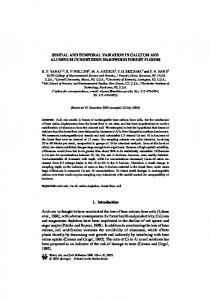
absence of a threshold).17 In addition, mean annual average GLO concentrations '20 parts per billion by volume (ppbv) are known to damage materials, concentrations '40 ppbv are known to damage crops and other seminatural vegetation, and concentrations '100 ppbv are known to damage trees.18 –20 Rural areas downwind of cities often experience higher GLO concentrations because of the advection of GLO and precursor gases from urban sources. Additionally, there is greater diurnal NO titration of GLO in urban areas compared with rural environments, which further depresses the urban:rural GLO ratio.3 Rural areas tend to have a greater proportion of the population who spend more time outdoors because of their occupation, typically in agriculture, forestry, or tourism. Therefore there is potential for higher exposure to GLO and a subsequent increased health burden in some sectors of the rural population compared with urban counterparts.16 Within Nova Scotia there is sufficient monitoring to observe and predict regional-scale GLO trends. However, the regional monitors cannot provide the finer scale detail needed to explore the spatiotemporal differences in GLO because of complex topography and local climatology such as exists in the Annapolis Valley. The regional monitors have shown that rural Nova Scotia often experiences mean 24-hr GLO concentrations in excess of 65 ppbv in the spring and summer months. Levels of GLO are therefore a cause of concern in this region. Consequently, the goals of this study were twofold: (1) to characterize using passive diffusion samplers the spatiotemporal variation of GLO in the rural Annapolis Valley, Nova Scotia (relative to more regionally representative sites such as Kejimkujik National Park, Nova Scotia), and hence to determine the exposure to GLO of the Annapolis Valley population and the potential harm to ecosystems, agriculture, and forestry on which the local economy depends; and (2) to investigate and model the relationships between meteorology and elevation on GLO concentrations in the region and between ambient and indoor GLO concentrations. The only previous data on GLO in the Annapolis Valley were for a single monitoring period between August 9 and September 6, 2000.21 MATERIALS AND METHODS Study Region The rural Annapolis Valley, Nova Scotia extends for 130 km from the town of Digby in the southwest end of the Valley to the town of Wolfville at the northeast end (Figure 1). The topography of the Annapolis Valley has the form of a “long thin funnel,” 10 km wide at the SW end and almost 20 km wide at the NE end, with the narrowest section only 5 km wide.21 The hills along the northwest and southeast sides of the Valley are referred to as North Mountain and South Mountain, respectively. The locations of the passive sampler (PS) and continuous automatic ozone analyzer monitoring sites are also shown in Figure 1, with additional site data provided in Table 1. Samplers were exposed at 17 locations, on up to 18 consecutive occasions between August 29, 2006 and September 28, 2007, between 14 and 28 days for each exposure. The PS sites were selected so as to include two cross-Valley Journal of the Air & Waste Management Association 311
Gibson et al.
Figure 1. PS and continuous ozone analyzer ambient and indoor monitoring locations in this study in the Annapolis Valley, Nova Scotia.
transects to investigate the variation in GLO concentrations with elevation. One transect passed close to the town of Middleton, midway along the Annapolis Valley, with the other passing through the town of Kentville toward the northeast end of the Valley. To assess PS precision, samplers were deployed in replicate throughout the measurement campaign at three of the monitoring locations: site 1 (duplicate), Kejimkujik, Environment Canada, Canadian Air and Precipitation Monitoring Network (CAPMoN); site 9 (triplicate), North Mountain, National Air Pollution Surveillance (NAPS) network; and site 12 (triplicate), Kentville (NAPS). The same three sites were each equipped with a Thermo Electron Instruments, Inc. model 49C continuous ozone analyzer that was used to assess PS accuracy. The indoor site was located in an air-conditioned open-plan office in the Centre of Geographic Sciences (COGS) at the Nova Scotia Community College Middleton Campus, 1.6 km north of the town of Middleton and 300 m from site 5 on the Annapolis Valley floor. Air conditioning was on all year to provide a constant temperature of approximately 20 °C. Windows were not opened during monitoring. The air-exchange rate was not measured. A standard suite of meteorological data was obtained from Environment Canada for one elevated location (site 1) and one Valley floor location (Greenwood, near site 5). GLO Determination Ogawa passive ozone diffusion samplers were used in this study (Ogawa & Co. USA Inc.). This design of sampler has been used in many studies investigating ambient, indoor, and personal exposure to GLO.22,23 The advantage of PS over continuous analyzers is that they require no power, are easy to deploy, are inexpensive, and offer the ability to carry out monitoring over a wide spatial area. The design and operation of the Ogawa sampler has been described in detail elsewhere23–25; however, in brief, for ambient 312 Journal of the Air & Waste Management Association
field monitoring the PS badge is attached onto a suitable upright or clipped into a weather shelter. In this study, Ogawa polyvinyl chloride weather shelters were used at the outdoor sites. For the indoor location the PS was suspended from the central point of the ceiling on a piece of string approximately 25 cm in length. These were attached to a stake or other upright at a height of 2.5 m and as far away from vegetation as possible. Ozone present in the atmosphere diffuses at a known constant rate (21.8 cm3 ! min%1) onto sodium-nitrite-impregnated filter pads within the badge, where it oxidizes the nitrite (NO2%) to nitrate (NO3%). At the end of the exposure period the NO3% is extracted from the filter pads with a known volume of water and quantified by ion chromatography (IC).26 Ogawa recommends an approximate 28-day limit for ambient PS measurements and longer if NO2% is still available for oxidation by GLO. IC analysis confirmed that there was a considerable amount of NO2% still available for reacting with GLO on all of the sample filters, thus ensuring no sample breakthrough occurred in this study. The average GLO concentration during the sampling period (which in this study ranged between 14 and 28 days) was then derived using the equation presented by Koutrakis et al.25 and reproduced below in eq 1.
O 3 (ppbv) !
Q"L D"A"t
(1)
where Q is the NO3% concentration ((g ! mL%1), L is the extraction volume (mL), D is the ozone collection rate (21.8 cm3 ! min%1), A is 0.0409 ((mol ppb ! m3), and t is the exposure time (min). In this work, NO3% was extracted from the filters with 5 mL of 18-M) water according to Ogawa protocols26 and determined using a Metrohm 761 IC instrument with autosampler. A Phenomenex Star Ion A300 (4.6 mm $ Volume 59 March 2009
Gibson et al. Table 1. Sampling site descriptions and x, y, and z coordinates.a
Sample Site Name and Description of Location
Site Code
Date Monitoring Began
Kejimkujik National Park, CAPMoNb 45 km to the southwest of the Annapolis Valley
1
February 8, 2007
Annapolis Royal
2
October 10, 2006
Middleton Transect, South Mountain
3
August 29, 2006
Middleton Transect, below South Mountain
4
August 29, 2006
Middleton Transect, below North Mountain
5
August 29, 2006
Middleton Transect, valley side of North Mountain ridge Middleton Transect, ocean side of North Mountain ridge Middleton Transect, coastal location on North Mountain North Mountain NAPSb
6
August 29, 2006
7
August 29, 2006
8
August 29, 2006
9
August 29, 2006
Thomas Brook
10
September 19, 2006
Kentville Transect, South Mountain
11
December 15, 2006
Kentville, NAPSb
12
August 29, 2006
Sheffield Mills Agriculture Research Station, Valley floor Kentville Transect, valley side of North Mountain ridge Kentville Transect, ocean side of North Mountain ridge Halls Harbour
13
January 9, 2007
14
December 15, 2006
15
December 15, 2006
16
December 15, 2006
Wolfville
17
October 10, 2006
COGS office, Nova Scotia Community College, Middleton Campus, Valley floor
Indoor (near site 5)
August 29, 2006
Coordinates, (Latitude: Longitude)
Elevation (m)
44° 26* 9.9+ %65° 12* 20.9+ 65° 12* 20.9+ 44° 44* 35.5+ %65° 30* 39.3+ 44° 51* 46.1+ %65° 2* 2.7+ 44° 54* 38.5+ %65° 4* 23.1+ 44° 57* 13.2+ %65° 4* 44.4+ 44° 58* 57.0+ %65° 6* 44.3+ 44° 58* 47.6+ %65° 5* 21.6+ 45° 0* 18.3+ %65° 7* 6.5+ 45° 4* 34.5+ %64° 50* 43.8+ 45° 3* 54.3+ %64° 45* 1.9+ 45° 2* 2.1+ %64° 29* 20.8+ 45° 4* 0.0+ %64° 28* 59.9+ 45° 7* 49.5+ %64° 29* 24.7+ 45° 9* 27.5+ %64° 32* 54.5+ 45° 10* 7.3+ %64° 34* 5.4+ 45° 11* 42.5+ %64° 36* 50.5+ 45° 5* 23.8+ %64° 22* 11.4+ 44° 57* 14.1+ %65° 4* 39.6+
Number of PS per Deployment
Classification
125
2
5
1
Wilderness elevated site Coastal
181.5
1
Valley top
26.8
1
Valley floor
26.9
1
Valley floor
165.5
1
Valley top
155.9
1
Valley top
81.2
1
Coastal
237.4
3
Valley top
31.4
1
Valley floor
217.0
1
Valley top
49
3
Valley floor
22.8
1
Valley floor
195.4
1
Valley top
145.9
1
Valley top
52.4
1
Coastal
37.8
1
Valley floor
26
1
Indoor
Notes: aAll sites are ambient except for one site near site 5, which is indoors; bContinuous GLO monitors present.
100 mm $ 7.5 (m; catalog no. 000-4090-EO-BV) analytical column and Phenomenex star-ion anion guard cartridge (10 $ 4.6 mm; catalog no. KH0-3112) were used. The eluant comprised 1.8 mM sodium carbonate (Na2CO3) mixed with 1.7 mM sodium bicarbonate (NaHCO3) in water, and the regenerant composition was a 0.020 M sulfuric acid (H2SO4) in water. The flow rate was 1.5 mL ! min%1. The instrument NO3% limit of detection (based upon three times the standard deviation [SD] of 5 blanks) for the 18 batches analyzed ranged from 0.5 to 0.9 mg ! L%1, which was well below the NO3% collected in the field samples. PS and blanks from the same batch of filters pads were assembled, transported, disassembled, and analyzed together. All PS and blanks were kept in a cool place (but not in a refrigerator or frozen) until required for IC analysis. Twenty percent of the samplers from each batch were used as field blanks. All samples were blank subtracted. Volume 59 March 2009
The PS detection limit, on the basis of analysis of the field blanks, was determined to be 0.8 ! 0.02 ppbv for a 14-day sampling period. This was far lower than the minimum sample value of 7.7 ppbv and 70 times lower than the annual mean measured GLO concentration of 34.3 ppbv. RESULTS AND DISCUSSION PS Validation PS replication was undertaken at sites 1 (n " 2), 9 (n " 3), and 12 (n " 3). For sites 9 and 12, the means of two of the three samplers, chosen at random, were compared with the remaining sampler. The PS intercomparison demonstrated excellent correlations with R2 values of 0.88 (n " 11), 0.95 (n " 17), and 0.96 (n " 17), respectively; and linear relationships not significantly different from 1:1 for GLO concentrations spanning the range of 25– 60 ppbv. From these data, an imprecision value (Sc) of only 5.4% was calculated for the PS in this study using the equation, Journal of the Air & Waste Management Association 313
Gibson et al. Sc " SD(#)/,2, where SD(#) is the SD of the percentage difference between duplicate measurements. Figure 2 shows the comparisons between exposureaveraged continuous analyzer and PS replicate mean GLO concentrations at sites 1, 9, and 12, which likewise showed very strong correlations with R2 values of 0.95
Figure 2. Intercomparisons between exposure-averaged ozone measurement by PS and continuous analyzer at three sites: (a) site 1, Kejimkujik; (b) site 9, North Mountain; and (c) site 12, Kentville. RMA, reduced major axis regression, which is an alternative to y-on-x least squares regression and allows for uncertainty in both the x and y data values.39 314 Journal of the Air & Waste Management Association
(n " 11), 0.82 (n " 17), and 0.95 (n " 13), respectively. (The continuous analyzer at site 12 was out of operation for several months, which accounts for the lower value of n in this intercomparison compared with the duplicate PS intercomparison above). The linear regression between PS and automatic analyzer was not significantly different from unity for sites 1 and 9 and close to unity for site 12. It was discovered that there was some slight negative calibration drift of the automatic analyzer at site 12. This probably accounts for the lower systematic GLO automatic analyzer measurements compared with the PS at site 12. However, overall, the accuracy intercomparison across all three sites is highly acceptable and compares favorably with Krupa et al.,14 who also showed good agreement (R2 values of 0.93 and 0.93) between Ogawa PS ozone and continuous ozone analyzer at two sites. Overall the PS validation study shows that the PS is accurate and precise over the range of GLO concentrations measured. SUMMARY OF GLO OBSERVATIONS The descriptive statistics for the observed GLO concentrations obtained over the course of the study from August 29, 2006 to September 28, 2007 are shown in Table 2 and are based on a total of 353 measurements (excluding blanks) comprising 335 ambient and 18 indoor measurements. Figure 3 summarizes the data at each monitoring location as box-whisker plots. Because the monitoring sites were not commissioned at the same time, direct comparison of descriptive statistics between sites requires some caution (refer to Table 1 for the sampling session dates). A time series of all of the observed GLO concentrations is shown in Figure 4. Comparison of Figures 3 and 4 shows that the GLO concentrations above the 90th percentile in Figure 3 are generally associated with a single exposure period, May 3 to May 17, 2007, whereas those below the 10th percentile are generally associated with the exposure periods August 29, 2006 to September 19, 2006, and September 19, 2006 to October 10, 2006. Figures 3 and 4 clearly illustrate the significantly lower indoor ozone concentrations compared with ambient GLO (P - 0.000). A one-way ANOVA with post-hoc Tukey’s pairwise comparisons was used to determine if there was a significant difference between the GLO concentrations observed between and within the 17 ambient sampling sites over the 18 sampling sessions. The results showed that the within-site GLO observations were significant (P - 0.001). Additionally, the Valley bottom sites (4, 5, and 10) were significantly different (P " 0.032) from site 7 on the North Mountain Ridge (Bay of Fundy side) and sites 3 and 11 on the South Mountain. However, sites 13, 12, and 17, toward the northeast end of the Valley floor, and the remaining coastal and mountain top sites were not significantly different from each other. To conclude, the GLO concentrations centered longitudinally along the Valley floor, are significantly less than those on the Valley floor near the northeast and southwest ends of the Valley. Volume 59 March 2009
Gibson et al. Table 2. Summary descriptive statistics of PS ozone sampling measurements for all 18 sites for the period August 29, 2006 to September 28, 2007.
Location Ambient (all sites) Valley floor Mountain top Coastal Wilderness elevated site (Kejimkujik National Park) Indoor site
n (including replicates)
Mean ! " (ppbv)
SE Mean (ppbv)
Min:Max (ppbv)
Skewness
Kurtosis
353 135 146 50
34.3 ! 10.1 29.9 ! 8.6 35.4 ! 9.9 35.4 ! 10.5
0.5 0.7 0.8 1.5
7.7:72.1 16.6:44.3 21.2:62.9 22.2:66.4
0.6 0.3 1.2 1.6
0.4 %0.9 2.2 3.5
22 18
33.8 ! 4.8 5.4 ! 3.3
1.0 0.8
27.0:41.3 1.3:13.0
0.3 .0
%1.0 0.5
Exploration of Spatiotemporal Trends Figure 4 clearly shows that the GLO concentrations observed at all of the ambient sampling sites follow a similar trend. The grouped mean (!1 SD) GLO concentration for the 6 Valley floor sites over the 13 months of monitoring was 30.9 ! 8.7 ppbv (n " 99), for the 7 elevated sites on the North and South Mountains it was 36.3 ! 9.6 ppbv (n " 65), and for the three coastal sites it was 36.4 ! 10.7 ppbv (n " 50). This compares with historical annual average GLO values at site 9 (North Mountain) in the range of 29.6 – 40.5 ppbv from 1996 to 2006 and annual mean GLO concentrations at Canadian background stations between 23 and 34 ppbv.27 Therefore, although the annual mean GLO concentrations determined on the Annapolis Valley floor fall within the range of Canadian background annual mean GLO levels, annual mean GLO levels at the elevated sites are higher.27 The maximum exposure-average concentration of 72 ppbv measured in this study was at site 6 on the North Mountain, for the period May 3–17, 2007. This concentration is above the typical mean background northern hemisphere springtime maximum GLO concentration of 60 ppbv measured over the last couple of decades.27–29 The remaining monitoring sites also experienced their highest GLO concentration during this period, which is related to the “spring max” often observed in the Annapolis Valley at this time of year (typically found over a
Figure 3. Box-whisker plot of observed passive GLO concentrations at each sampling location for the sampling campaign August 29, 2006 to September 28, 2007. Volume 59 March 2009
couple of weeks between mid-April to the end of May). The time when the GLO spring maximum appears varies around the globe and is dependent upon latitude, elevation, availability of ozone precursors, temperature, and solar radiation intensity.2 The spring max may be explained by several factors. There is evidence of springtime stratospheric-tropospheric exchange driven by the Brewer– Dobson circulation, although this is not believed to be the main contributor to the springtime maximum.29 One of the more important reasons for the springtime maximum in the northern hemisphere is buildup of peroxyacetyl nitrate (PAN), non-methane VOCs, and carbon monoxide (CO), together with seasonal emissions of biogenic isoprene, which, coupled with increased solar radiation and temperature, lead to a predominately photochemically driven spring maximum.30 –32 Furthermore, there is also an increase in water vapor observed during this period, which leads to an increase in the hydroxyl radical concentration and hence again to an increase in photochemical ozone generation.30 Finally, warmer temperatures increase lightening activity and soil microbial activity, which in turn lead to increased NO2 emissions from these sources. The springtime maximum is increasing in the northern hemisphere (has roughly doubled in
Figure 4. Time-series plot of ambient and indoor GLO concentrations, Annapolis Valley, Nova Scotia, from August 29, 2006 to September 28, 2007. AA " sites with a colocated continuous automatic ozone analyzer. Journal of the Air & Waste Management Association 315
Gibson et al. the past 10 yr) compared with the southern hemisphere, which is thought to be driven mainly by the increasing anthropogenic emissions of ozone precursors.29 To help interpret more specifically the elevated GLO concentration observed over the period May 3–17, 2007, and the subsequent reduction during the following sampling period, May 17 to June 6, 2007, wind direction and wind speed frequency plots (wind roses) were constructed for both periods (using the meteorological data from Greenwood) and shown in Figure 5a and b, respectively. As can be seen in Figure 5a, the average airflow for the period May 3–17, 2007, was from the west-northwest (296°) vector, with the highest wind speeds associated
Figure 5. Wind rose plots showing wind direction and wind speed frequency for the sampling sessions (a) May 3–17, 2007 and (b) May 17–June 6, 2007. 316 Journal of the Air & Waste Management Association
with the west-southwest (252°) vector. Three-day air mass back trajectories (AMBTs) obtained from Environment Canada confirmed the wind rose analysis. Wind from the west-southwest direction passes over strong sources of ozone precursors in the northeastern United States and the Windsor–Quebec corridor in southeastern Canada. The airflow over known source areas, coupled with the seasonal burst in biogenic VOC emissions and warmer seasonal temperatures, very likely accounts for the elevated GLO observed from May 3–17, 2007. This period requires further study and will be looked at in the future because it is beyond the scope of this paper. As can be seen in Figure 5b, the average wind direction, again confirmed by AMBT, for the May 17 to June 6, 2007, period was from the north-northeast (8°), with the highest wind speeds predominately from the clean North Atlantic sector. As can be seen in Figure 4, this also coincides with a sharp decrease in GLO concentrations in the Annapolis Valley. The sharp decline in the observed GLO during this period is therefore likely due to the significant change in dominating meteorology compared with the previous sampling session and the reduction in the wintertime reservoir of PAN, CO, and non-methane hydrocarbons. This period also coincides with the rapid emergence of vegetation in this region, which increases surface deposition and uptake of GLO through plant stomata.3 Additional analysis of the meteorological data shows that the weather was damper and cooler (1 °C below normal) during this period, which may also have contributed to the decline in GLO. The increase in the ozone concentration observed between August 30, 2007 and September 28, 2007 was probably enhanced by the record breaking temperatures (maximum 31.4 °C, mean 16.1 °C) favoring photochemical formation of GLO, compared with the same period in 2006 (maximum 26.2 °C, mean 13.6 °C). Additionally, wind rose analysis showed that the airflow during this period was from the west with the strongest winds associated with west-southwest airflow from known source areas in southeastern Ontario. Three-day AMBT analysis confirmed the local wind direction measurements.
Comparison of Mountain, Coastal, and Valley Floor Sites Figure 6 is a plot of the mean GLO concentrations observed at the coastal sites (2, 8, and 16), mountain tops (1, 3, 6, 7, 9, 11, 14, and 15), valley floor sites (4, 5, 10, 12, 13, and 17) and the indoor location. There is a clear trend for GLO along the Valley floor to be lower than at the coast or at higher elevations. Research by Coyle et al.3 implicated ozone-enriched air flowing from the ocean as a factor in favor of the higher ozone concentrations at coastal sites in the United Kingdom. Ozone concentrations are often higher over the sea and large lakes than over adjacent land because of inefficient dry deposition to the former surface. It is also thought that the effect of cloud suppression enhancing ultraviolet photochemistry leading to mean higher GLO Volume 59 March 2009
Gibson et al. The strong quantitative relationship (R2 " 0.82) between elevation and mean GLO concentration over the period December 15, 2006 to September 28, 2007 for the sites along the two cross-valley transects is illustrated in Figure 7. (Some of the sites were not established before this date and would therefore bias the comparison.) The coastal sites have been excluded from Figure 7 because of the influence of onshore ocean breezes on these sites.3 This relationship will be studied further but is outside the scope of this paper. Multivariate Model of GLO Estimation Numerous studies have investigated the use of meteorological variables as a means of predicting GLO concentrations.14,35 According to the National Research Council, one method to estimate GLO is to use meteorological indicators in the general form of eq 2: GLO " (exp.a/).TEMP/b.WS/c.RH/d.SKY/e Figure 6. Time-series plot of the mean GLO concentrations per sampling period observed at the coastal sites, mountaintop sites, Valley floor sites, and the indoor location.
concentrations over the ocean and large lakes compared with adjacent land may also explain higher GLO concentrations at the coast.33 This is the likely explanation for the higher concentrations observed at either end of the Annapolis Valley, where onshore flows from the Annapolis Basin in the southwest and the Minas Basin in the northeast could result in higher ozone concentrations at the coastal sites. This probably also explains the slightly higher GLO concentrations observed at the Valley floor at the northeast and southwest extremes of the Annapolis Valley (sites 2, 13, 12, and 17) compared with Valley floor sites further within the Valley. These sites are closer to the ocean and are more likely to be influenced by daytime onshore breezes advecting ozone-rich marine air into this area, causing a slight increase in the GLO concentrations compared with the longitudinal center of the Valley, the GLO concentrations of which differ significantly from the coast and mountaintops. The higher GLO concentrations observed, on average, on the mountains on either side of the Valley compared with the Valley floor are consistent with previous observations elsewhere.3 This observation is highly likely because of the flow of colder air into the Valley bottom at night (drainage), which is then replaced by relatively ozone-rich air from above through the generally greater turbulence fluxes at night at elevations than in the more stratified nighttime air of the Valley floor. The Valley floor air is also subject to greater stomatal and non-stomatal vegetation uptake and NO titration from local combustion sources.34 Additionally, the elevated sites have more frequent exposure to the free troposphere and to the pollutant plumes that are transported aloft from their places of origin to the south and west of the region. Volume 59 March 2009
(2)
where TEMP is the temperature, WS is the wind speed, RH is relative humidity, SKY represents the sky cover or solar radiation, and a–e are fitted constants. Other variables considered include wind direction, dew point temperature, sea level pressure (elevation), and precipitation.14 In the case of passive sampling these meteorological variables are calculated as averages over the duration of each sampling period. Environment Canada has used a nonparametric data-driven tree-based analysis method known as CART (classification and regression trees) to predict daily maximum GLO for the Vancouver, Montreal and Atlantic Regions of Canada.36 The CART analysis used the following meteorological predictors of GLO: maximum GLO yesterday, maximum temperature, dew point, relative humidity (RH), surface wind speed and direction, surface pressure, sunshine, precipitation, thunderstorm activity, haze, synoptic class, day of the week, and dry convective mixing height.36
Figure 7. Relationship between elevation and mean ambient GLO concentrations from December 15, 2006 to September 28, 2007 (site locations shown). RMA " reduced major axis regression. Journal of the Air & Waste Management Association 317
Gibson et al. A multivariate model was developed for this study to predict GLO on the Valley floor, near site 5, on the basis of the mean meteorological data obtained from the nearby weather station at Greenwood. The meteorological parameters included visibility, wind direction, wind speed, temperature, RH, cloud opacity and cloud amount (latter two metrics measured by a Meteorological Service Canada trained observer). The ‘best subsets’ tool in Minitab version 15 (Minitab Inc. US, 2008) was used to select the following optimum meteorological parameters that best described the observed GLO, as judged by the criteria of lowest Mallows (Cp) value, highest R2 value and least number of variables: visibility, wind direction, wind speed, temperature, and RH. Using the regression tool in Minitab 15, the multivariate model given in eq 3 was developed to predict GLO on the floor of the Annapolis Valley. GLO [ppbv] ! 162.5 # 3.910 # 0.00591 $ 2.71( $ 0.56ε # 1.252
(3)
where the constant 162.5 is the intercept, 0 is the visibility (km), 1 is the wind direction (degrees), ( is the wind speed (km ! hr%1), ε is the temperature (°C), and 2 is RH (%). The standard error (SE) and P values for the coefficients are as follows: constant (SE " 61.96), 0 (SE " 1.75, P " 0.046), 1 (SE " 0.021, P " 0.079), ( (SE " 0.77, P " 0.004), ε (SE " 0.29, P " 0.083), and 2 (SE " 0.44, P " 0.014). The model in eq 3 accounted for 87% (R2) of the variation in observed GLO on the Valley floor. The most important predictors of GLO derived from eq 3 are visibility, wind speed, and RH, with temperature and wind direction having borderline significance (P " 0.083 and P " 0.079, respectively). However, it is well know that temperature and wind direction are important predictors of GLO and should be considered in a model of this kind.14 The model used in eq 3 to predict GLO on the Valley floor was validated using meteorological data from the same site from January 9, 2004 to May 3, 2006 and covering the same sampling periods. The R2 between the observed and the predicted GLO for the Valley floor was 0.61, with a significance of 0.000. Thus the model in eq 3 is able to explain 61% of the GLO variance on the Valley floor. In a similar way, the multivariate model given in eq 4 was developed to predict GLO at elevated locations by using meteorological data obtained from site 1 (Kejimkujik, CAPMoN). Visibility data were not available for this model. GLO [ppbv] ! 84.1 # 0.00751 $ 1.34( # 0.137ε # 0.5532
Indoor Predictive Model Figure 8 shows the relationship between ambient GLO at site 5 on the Valley floor with indoor measurements nearby. A significant correlation (R2 " 0.71) exists between ambient and indoor ozone concentrations, suggesting a relationship. A predictive model for the latter from the former is given by eq 5. Indoor (ppbv) " (0.34 $ ambient (ppbv)) % 5.07
(5)
This model in eq 5 is based only on one indoor location and does not include air-exchange rate. Clearly studies of different types of housing in the Annapolis Valley with an assessment of air-exchange rate and ventilation modes are required to validate and improve the accuracy and general applicability of this model. Potential for Human and Environmental Health Effects The mean ambient GLO concentrations observed throughout the year of measurements at all of the sites in this study are sufficiently high to impact human health17 and to damage materials such as rubber.3 For the period
(4)
where the variables have the same meaning and units as above. The SE and P values for the coefficients for eq 4 are as follows: intercept (SE " 20.73, P " 0.001), 1 (SE " 0.05, P " 0.054), ( (SE " 1.02, P " 0.021), ε (SE " 0.15, P " 0.087), and 2 (SE " 0.17, P " 0.008). The model in eq 4 described 50% (R2) of the observed GLO compared with 318 Journal of the Air & Waste Management Association
87% (R2) in eq 3. The most important predictors that control GLO at the elevated Kejimkujik CAPMoN site (site 1) are RH and wind speed, with temperature and wind direction having borderline significance (P " 0.087 and P " 0.054, respectively). Again, the model used in eq 4 to predict GLO at the elevated location at site 1 (Kejimkujik National Park) was compared with meteorological data from January 9, 2004 to September 19, 2006. The R2 between the observed and the predicted GLO for this elevated location was 0.70, with a significance of 0.000. Thus the model in eq 4 is able to explain 70% of the GLO variance at site 1. The models shown in eqs 3 and 4 compare very favorably with the model developed by Krupa et al.,14 which explained 62.5– 67.5% (R2) of the GLO variance in Moshannon State Forest in Pennsylvania.14
Figure 8. Comparison between ambient (site 5) and indoor (near site 5) passive GLO measurements on the Valley floor. Volume 59 March 2009
Gibson et al. from February 8 to May 17, 2007, the mean GLO concentration across the 17 sampling sites exceeded 40 ppbv, which is known to have a negative impact on vegetation.20 Trees would exhibit some stress and possible emerging leaf damage during the period spanning the May 3–17, 2007, in which the mean GLO was 56 ppbv.37 The springtime average and episodic GLO values observed in this study can be compared with the annual mean Canadian background of between 23 and 34 ppbv, and a global clean tropospheric background of between 20 ppbv in the winter and 60 ppbv in the summer.27 Under a warming climate, one potential effect may be for vegetation to emerge earlier, which would coincide with the highest annual GLO concentrations. If this were to happen, there is substantial risk of increased vegetation damage caused by GLO.38 CONCLUSIONS This study has demonstrated that Ogawa PS analyzers are a useful tool with which to conduct long-term studies of GLO over a wide geographic area and has highlighted the effect of topography and meteorology on seasonal GLO concentrations in this rural region. The models described in this paper are an effort to extend the utility of the time-integrated PS ozone data toward the parameterization of ambient GLO in the region. Additionally, the model developed to predict indoor GLO concentrations from corresponding ambient measurements may also prove useful in estimating exposures to GLO in indoor microenvironments. The GLO concentrations experienced in the study are known to cause damage to health, materials, vegetation, and agricultural crops, especially to the latter in the spring during vegetation emergence. The data collected in this study will be useful in predicting the damage to vegetation and crops in the rural Annapolis Valley, Nova Scotia, Canada. Finally, the insights and knowledge gained from this study of ambient rural community-scale exposure will enhance our understanding of current and future epidemiological personal exposure studies in the region related to GLO (and other air quality metrics) in rural and urban settings. ACKNOWLEDGMENTS This work was supported by Canadian Institutes of Health Research (CIHR) grant(s) Centre for Research Development, Grant 62398 –Atlantic RURAL Centre. The authors would like to acknowledge Environment Canada, Air Quality Science Section in Dartmouth, Nova Scotia for funding the project, for supplying continuous automatic ozone analyzer, meteorological, and back trajectory analysis data. The authors are indebted to David Colville, Jeff Wentzell, and Darren McKinnon at the Applied Geomatics Research Group and Centre of Geographic Sciences of Nova Scotia Community College Middleton Campus for providing site access and for assisting with the field work. The authors thank Nova Scotia Environment, Air Quality Section for providing additional funding support. The authors also thank Fran Di Cesare, Nova Scotia Environment, Air Quality Section for supplying further continuous automatic ozone analyzer data. In addition, the Volume 59 March 2009
authors thank Peter Romkey of the K.C. Irving Environmental Science Centre, Acadia University; Steve Hawbolt of the Clean Annapolis River Project; Deborah Veinot, site operator, Kejimkujik CAPMoN; and Dr. John Eustace, Giselle Eustace, and David Lacey for their assistance with providing sampling sites and sampler deployment. Finally, the authors thank Perkin-Elmer Instruments, Inc., for supporting our research activity. REFERENCES
1. Rao, S.T.; Zurbenko, I.G. Detecting and Tracking Changes in Ozone Air Quality; J. Air & Waste Manage. Assoc. 1994, 44, 1089-1092. 2. Finlayson-Pitts, B.J.; Pitts, J.N. Chemistry of the Upper and Lower Atmosphere; Academic: New York, 1999. 3. Coyle, M.; Smith, R.I.; Stedman, J.R.; Weston, K.J.; Fowler, D. Quantifying the Spatial Distribution of Surface Ozone Concentration in the UK; Atmos. Environ. 2002, 36, 1013-1024. 4. Kim, S.-W.; Heckel, A.; McKeen, S.A.; Frost, G.J.; Hsie, E.-Y.; Trainer, M.K.; Richter, A.; Burrows, J.P.; Peckham, S.E.; Grell, G.A. SatelliteObserved U.S. Power Plant NOx Emission Reductions and their Impact on Air Quality; Geophys. Res. Lett. 2006, 33, doi: 10.1029/ 2006GL027749. 5. Lefohn, A.S.; Oltmans, S.J.; Dann, T.; Singh, H.B. Present-Day Variability of Background Ozone in the Lower Troposphere; J. Geophys. Res. 2001, 106, 9945-9958. 6. Wu, S.; Mickley, L.J.; Jacob, D.J.; Logan, J.A.; Yantosca, R.M.; Rind, D. Why Are there Large Differences between Models in Global Budgets of Tropospheric Ozone?; J. Geophys. Res. 2007, 112, doi: 10.1029/ 2006JD007801. 7. Martin, R.V.; Fiore, A.M.; Van Donkelaar, A. Space-Based Diagnosis of Surface Ozone Sensitivity to Anthropogenic Emissions; J. Geophys. Res. 2004, 31, doi: 10.1029/2004GL019416. 8. Gong, W.; Mickle, R.E.; Bottenheim, J.; Froude, F.; Beauchamp, S.; Waugh, D. Marine and Coastal Boundary Layer and Vertical Structure of Ozone Observed at a Coastal Site in Nova Scotia during the 1996 NARSTO-CE Field Campaign; Atmos. Environ. 1999, 34, 4139-4154. 9. Johnson, D.; Mignacca, D.; Herod, D.; Jutzi, D.; Miller, H. Characterization and Identification of Trends in Average Ambient Ozone and Fine Particulate Matter Levels through Trajectory Cluster Analysis in Eastern Canada; J. Air & Waste Manage. Assoc. 2007, 57, 907-918. 10. Fehsenfeld, F.C.; Daum, P.; Leitch, W.; Trainer, M.; Parrish, D.; Hubler, G. Transport and Processing of O3 and O3 Precursors over the North Atlantic: an Overview; J. Geophys. Res. 1996, 101, 28,877-28,891. 11. Li, Q.B.; Jacob, D.J.; Park, R.; Wang, Y.X.; Heald, C.L.; Hudman, R.; Yantosca, R.M.; Martin, R.V.; Evans, M.J. Outflow Pathways for North American Pollution in Summer: a Global 3-D Model Analysis of MODIS and MOPITT Observations; J. Geophys. Res. 2005, 110, doi: 10.1029/2004JD005039. 12. Tordon, R.; George, P.; Beauchamp, S.T; Keddy, K. Source Sector Analysis of Ozone Exceedance Trajectories in the Maritime Region (1980 –1993); MAES 2-94; Environment Canada; Atmospheric Environment Service: Gatineau, Quebec, Canada, 1994. 13. Lin, C.-H. Impact of Downward-Mixing Ozone on Surface Ozone Accumulation in Southern Taiwan; J. Air & Waste Manage. Assoc. 2008, 58, 562-579. 14. Krupa, S.; Nosal, M.; Ferdinand, J.A.; Stevenson, R.E.; Skelly, J.M. A Multi-Variate Statistical Model Integrating Passive Sampler and Meteorology Data to Predict the Frequency Distributions of Hourly Ambient Ozone (O3) Concentrations; Environ. Pollut. 2003, 124, 173-178. 15. Stieb, D.M.; Judek, S.; Burnett, R.T. Meta-Analysis of Time-Series Studies of Air Pollution and Mortality: Effects of Gases and Particles and the Influence of Cause of Death, Age, and Season; J. Air & Waste Manage. Assoc. 2002, 52, 470-484. 16. Brauer, M.; Brook, J.R. Ozone Personal Exposures and Health Effects for Selected Groups Residing in the Fraser Valley. The Lower Fraser Valley Oxidants/Pacific ’93 Field Study; Atmos. Environ. 1997, 31, 2113-2121. 17. Bell, M.L.; Peng, R.D.; Dominici, F. The Exposure-Response Curve for Ozone and Risk of Mortality and the Adequacy of Current Ozone Regulations; Environ. Health Perspect. 2006, 114, 532-536. 18. Percy, K.E. New Exposure-Based Metric Approach for Evaluating O3 Risk to North American Aspen Forests; Environ. Pollut. 2007, 147, 554-566. 19. Lee, D.S.; Cape, J.N.; Cupit, M.; Derwent, R.G.; Falls, N.A.R.; Holland, M.R.; Lewis, P.M.; Mower, K.G. The Effects of Ozone on Materials: First Six-Monthly Progress Report to the Department of the Environment, December 1995; Contract EPG 1/3/50; AEA Technology Ltd.: Aberdeen, UK, 1995. 20. Krupa, S.; Nosal, M.; Peterson, D.L. Use of Passive Ozone (O3) Samplers in Vegetation Effects Assessment; Environ. Pollut. 2001, 112, 303-309. Journal of the Air & Waste Management Association 319
Gibson et al. 21. Waugh, D.L.; Mehlman, S. Report on the Annapolis Valley Ground Level Ozone Field Experiment—Summer 2000; Atlantic Region Science Report Series 2004-01; Meteorological Service of Canada: Ottawa, Ontario, Canada, 2004. 22. Geyh, A.S.; Roberts, P.T.; Lurmann, F.W.; Schoell, B.S.; Avol, E.L. Initial Field Evaluation of the Harvard Active Ozone Sampler for Personal Ozone Monitoring; J. Environ. Anal. Environ. Epidemiol. 1999, 2, 143-149. 23. Karthikeyan, S.; Sundararajan, V.S.; Balasubramanian, R.; Zuraimi, M.S.; Tham, K.W. Determination of Ozone in Outdoor and Indoor Environments Using Nitrite-Impregnated Passive Samplers followed by Ion Chromatography; J. Air & Waste Manage. Assoc. 2007, 57, 974-980. 24. Brauer, M.; Brook, J.R. Personal and Fixed-Site Ozone Measurements with a Passive Sampler; J. Air & Waste Manage. Assoc. 1995, 45, 529537. 25. Koutrakis, P.; Wolfson, J.M.; Bunyaviroch, A.; Froehlich, S.E.; Hirano, K.; Mulik, J.D. Measurement of Ambient Ozone Using a Nitrite-Coated Filter; Anal. Chem. 1993, 65, 209-214. 26. Ogawa Protocol for Ozone Measurement Using Ozone Passive Sampler Badge; Ogawa & Co. USA: Pompano Beach, FL, 2001. 27. Vingarzan, R. A Review of Surface Ozone Background Levels and Trends; Atmos. Environ. 2004, 38, 3431-3442. 28. Bonasoni, P.; Stohl, A.; Cristofanelli, P.; Calzolari, F.; Colombo, T.; Evangelisti, F. Background Ozone Variations at Mt. Cimone Station; Atmos. Environ. 2000, 34, 5183-5189. 29. Monks, P.S. A Review of the Observations and Origins of the Spring Ozone Maximum; Atmos. Environ. 2000, 34, 3545-3561. 30. Choi, Y.; Wang, Y.; Zeng, T.; Cunnold, D.; Yang, E.-S.; Martin, R.; Chance, K.; Thouret, V.; Edgerton, E. Springtime Transitions of NO2, CO, and O3 over North America: Model Evaluation and Analysis; J. Geophys. Res. 2008, 113, D20311, doi: 10.1029/2007JD009632. 31. Wang, Y.; Jacob, D.J.; Logan, J.A. Global Simulation of Tropospheric O3-NOx-Hydrocarbon Chemistry. 3. Origin of Tropospheric Ozone and Effects of Nonmethane Hydrocarbons; J. Geophys. Res. 1998, 103, 10757-10767. 32. Yienger, J.J.; Levy, H. Empirical Model of Global Soil-Biogenic NOx Emissions; J. Geophys. Res. 1995, 100, 11,447-11,464. 33. Sabburg, J.; Wong, J. The Effect of Clouds on Enhancing UVB Irradiance at the Earth’s Surface: a One Year Study; J. Geophys. Res. Lett. 2000, 27, 3337-3340. 34. Li, Q.; Jacob, D.J.; Bey, I.; Palmer, P.I.; Duncan, B.N.; Field, B.D.; Martin, R.V.; Fiore, A.M.; Yantosca, R.M.; Parrish, D.D.; Simmonds, P.G.; Oltmans, S.J. Transatlantic Transport of Pollution and Its Effects on Surface Ozone in Europe and North America; J. Geophys. Res. 2002, 107, doi: 10.1029/2001JD001422. 35. Abdul-Wahab, S.A.; Bakheit, C.S.; Al-Alawi, S.M. Principal Component and Multiple Regression Analysis in Modeling of Ground-Level Ozone and Factors Affecting Its Concentrations; Environ. Model. Software 2005, 20, 1263-1271. 36. Burrows, W.R.; Benjamin, M.; Beauchamp, S.; Lord, E.R.; McCollor, D.; Thomson, B. CART. Decision-Tree Statistical Analysis and Prediction of Summer Season Maximum Surface Ozone for the Vancouver, Montreal, and Atlantic Regions of Canada; J. Appl. Meteorol. 1995, 34, 1848-1862. 37. Bardo, D.N.; Chappelka, A.H.; Somers, G.L.; Miller-Goodman, M.S.; Stolte, K. Ozone Impacts on Loblolly Pine (Pinus Taeda l.) Grown in a Competitive Environment; Environ. Pollut. 2002, 116, 27-36. 38. Karlsson, P.E.; Tang, L.; Sundberg, J.; Chen, D.; Lindskog, A.; Pleijel, H. Increasing Risk for Negative Ozone Impacts on Vegetation in Northern Sweden; Environ. Pollut. 2007, 150, 96-106.
320 Journal of the Air & Waste Management Association
39. Heal, M.R.; Beverland, I.J.; McCabe, M.; Hepburn, W.; Agius, R.M. Intercomparison of Five PM10 Monitoring Devices and the Implications for Exposure Measurement in Epidemiological Research; J. Environ. Monitor. 2000, 2, 455-461.
About the Authors Mark Gibson is an environmental health and air pollution specialist holding a teaching faculty position in the Department of Community Health and Epidemiology, a senior research scientist with the Atlantic RURAL Centre, and an adjunct professor in the Department of Civil Engineering at Dalhousie University. Judy Guernsey is an associate professor in the Department of Community Health and Epidemiology at Dalhousie University and is director of the Atlantic RURAL Centre. Stephen Beauchamp is an atmospheric chemist and air quality science manager and David Waugh is an air quality meteorologist in the Air Quality Science Section of Environment Canada in Dartmouth, Nova Scotia. Mathew Heal is a senior lecturer in environmental chemistry, specializing in atmospheric and air quality measurements, in the School of Chemistry at the University of Edinburgh in Scotland. Jeffrey R. Brook is a senior research scientist in the Air Quality Research Division of Environment Canada. Robert Maher is a senior research scientist and Director of the Applied Geomatics Research Group (AGRG) and Centre of Geographic Sciences (COGS), at Nova Scotia Community College in Middleton, Nova Scotia. Graham Gagnon is an associate professor at the Department of Civil Engineering at Dalhousie University. Johnny McPherson is an air shed planner and Barbara Bryden is an air quality monitoring and reporting manager with the Air Quality Section of Nova Scotia Environment. Richard Gould is a medical officer of health with the Annapolis Valley Health Board in Wolfville, Nova Scotia. Mikiko Terashima is a Ph.D. candidate investigating the social determinants of health in the Department of Community Health and Epidemiology at Dalhousie University. Please address correspondence to: Mark Gibson, Room 401, Community Health and Epidemiology, Dalhousie University, 5790 University Avenue, Halifax, Nova Scotia, Canada B3H 1V7; phone: &1-902-412-1255; fax &1-902-4941597; e-mail:
[email protected].
Volume 59 March 2009