May 15, 2006 - arXiv:gr-qc/0605087v1 15 May 2006. Quantization of strings and branes coupled to BF theory. John C. Baez. Department of Mathematics,.
Quantization of strings and branes coupled to BF theory John C. Baez Department of Mathematics, University of California,
arXiv:gr-qc/0605087v1 15 May 2006
Riverside, CA 92521, USA. Alejandro Perez Centre de Physique Th´eorique, Unit´e Mixte de Recherche (UMR 6207) du CNRS et des Universit´es Aix-Marseille I, Aix-Marseille II, et du Sud Toulon-Var; laboratoire afili´e `a la FRUMAM (FR 2291), Campus de Luminy, 13288 Marseille, France. (Dated: February 4, 2008)
Abstract BF theory is a topological theory that can be seen as a natural generalization of 3-dimensional gravity to arbitrary dimensions. Here we show that the coupling to point particles that is natural in three dimensions generalizes in a direct way to BF theory in d dimensions coupled to (d − 3)branes. In the resulting model, the connection is flat except along the membrane world-sheet, where it has a conical singularity whose strength is proportional to the membrane tension. As a step towards canonically quantizing these models, we show that a basis of kinematical states is given by ‘membrane spin networks’, which are spin networks equipped with extra data where their edges end on a brane.
1
Interest in the quantization of 2 + 1 gravity coupled to point particles has been revived in the context of the spin foam [1] and loop quantum gravity [2] approaches to the nonperturbative and background-independent quantization of gravity. On the one hand this simple system provides a nontrivial example where the strict relation between the covariant and canonical approaches can be demonstrated [3]. On the other hand intriguing relationships with field theories with infinitely many degrees of freedom have been obtained [4]. The idea of generalizing this construction to higher dimensions is very appealing. We will argue that in 3 + 1 dimensions, the natural objects replacing point particles are strings. This idea has already been studied in a companion paper [5], which treated these strings merely as defects in the gauge field— i.e., places where it has a conical singularity. Here we propose a specific dynamics for the theory and a strategy for quantizing it. More generally, in d-dimensional spacetime we describe a way to couple (d − 3)-branes to BF theory. To understand this, first recall that in three dimensions, Einstein’s equations force the curvature to vanish at every point of spacetime. Therefore, except for global topological excitations, three-dimensional pure gravity does not have local degrees of freedom. However, it is precisely this local rigidity of Einstein’s gravity in three dimensions that makes it easy to couple the theory to point particles. The presence of massive point particles in three-dimensional gravity modifies the classical solutions by producing conical curvature singularities along the particles’ world-lines. With this idea in mind, one can write an action for a single particle coupled to gravity by introducing a source term to the standard action in the first order formalism, namely: Z Z S(A, e) = tr[e ∧ F (A)]) + m tr[e v], M
(1)
γ
where m is the mass of the particle, v is a fixed unit vector in the Lie algebra su(2), and γ is the world-line of the particle. It is easy to see that the previous action leads to equations of motion whose solutions are flat everywhere except for a conical singularity along γ, as desired. Unfortunately, this action suffers two drawbacks. First, it is no longer invariant under the standard gauge symmetries of pure gravity. Second, there is no explicit dependence on the particle degrees of freedom: one is describing the particle simply as a gauge defect along γ. One can solve both problems in one stroke by adding degrees of freedom for the particles, and choosing an action invariant under an appropriate extension of the gauge group of the 2
system. The result is the Sousa Gerbert action [6] for a spinless point particle of mass m coupled to three-dimensional Riemannian gravity: Z Z S(A, e, q, λ) = tr[e ∧ F (A)] + m tr[(e + dA q) λvλ−1]. M
(2)
γ
Here v is a fixed unit vector in su(2) as before, while the particle’s degrees of freedom are described by an su(2)-valued function q and an SU(2)-valued function λ defined on the worldline γ. The physical interpretation of q is a bit obscure, but we can think of it as ‘position in an internal space’. In a similar way, p = mλvλ−1 represents the particle’s momentum, which is treated as an independent variable in this first-order formulation. This action is invariant under the gauge transformations e 7→ geg −1 A 7→ gAg −1 + gdg −1
(3)
q 7→ gqg −1 λ 7→ gλ, where g ∈ C ∞ (M , SU(2)) and e 7→ e + dA η
(4)
q 7→ q − η,
where η ∈ C ∞ (M , su(2)). In addition to these gauge symmetries, the action is invariant under λ 7→ λh where h ∈ C ∞ (γ, H) and H ⊂ SU(2) is the subgroup consisting of elements g ∈ SU(2) that stabilize the vector v, meaning that gvg −1 = v. The action is also invariant under reparametrization of the world-line γ. A generalization of the naive action (1) to arbitrary dimensions can be constructed as follows. Let G be a Lie group such that its Lie algebra g is equipped with an inner product invariant under the adjoint action of G. Let M be a d-dimensional smooth oriented manifold equipped with an oriented (d −2)-dimensional submanifold W , which we call the ‘membrane world-sheet’. Let P be a principal G-bundle over M; to simplify the discussion we shall assume P is trivial, but this is not essential. One can define the action Z Z tr[B ∧ F (A)] + τ tr[B v] S(A, B) = M
(5)
W
where τ is the membrane tension, B is a g-valued (d − 2)-form, A is a connection on P , v is a fixed but arbitrary unit vector in g, and ‘tr’ stands for the invariant inner product in 3
g. The first term is the standard BF theory action, while the second is a source term that couples BF theory to the membrane world-sheet. As with the action in equation (1), the above action is only gauge-invariant if we restrict gauge transformations to be trivial on the membrane world-sheet. We can relax this condition by introducing appropriate degrees of freedom for the (d − 3)-brane whose world-sheet is W . The resulting action is: S(A, B, q, λ) =
Z
tr[B ∧ F (A)] + τ M
Z
tr[(B + dA q) λvλ−1],
(6)
W
where q is a g-valued (d − 3)-form on W and λ is a G-valued function on W . This action is invariant under the gauge transformations: B 7→ gBg −1 A 7→ gAg −1 + gdg −1 q 7→ gqg −1
(7)
λ 7→ gλ, where g ∈ C ∞ (M , G) and B 7→ B + dA η q 7→ q − η,
(8)
where η is any g-valued (d − 3)-form. As in the particle case, the action is also invariant under λ 7→ λh, where h ∈ C ∞ (W , H) and H ⊆ G is the subgroup stabilizing v, and under reparametrization of the membrane world-sheet. Perhaps the most intuitive equation of motion comes from varying the B field. This says that the connection A is flat except at W : F = −pδW ,
(9)
where p = τ λvλ−1 and δW is the distributional 2-form (current) associated to the membrane world-sheet. So, the membrane causes a conical singularity in the otherwise flat connection A. The strength of this singularity is determined by the field p, which plays the role of a ‘momentum density’ for the brane. Note that while the connection A is singular in the directions transverse to W , it is smooth and indeed flat when restricted to W . Thus the equation of motion obtained from varying q makes sense: dA p = 0. This expresses conservation of momentum density. 4
(10)
I.
THE CANONICAL ANALYSIS FOR d = 4
In this section we work out the other equations of motion as part of a canonical analysis of the action (6). But, in order to simplify the presentation, we restrict for the moment to the case d = 4—that is, the coupling of a string to four-dimensional BF theory. In Section III, we generalize the calculations to arbitrary dimensions. For this canonical analysis, we assume the spacetime manifold is of the form M = Σ × R. We choose local coordinates (t, xa ) for which Σ is given as the hypersurface {t = 0}. By definition, xa with a = 1, 2, 3 are local coordinates on Σ. We also choose local coordinates (t, s) on the 2-dimensional world-sheet W , where s ∈ [0, 2π] is a coordinate along the onedimensional string formed by the intersection of W with Σ. We pick a basis ei of the Lie algebra g, raise and lower Lie algebra indices using the inner product, and define structure constants by [ei , ej ] = ckij ek . Performing the standard Legendre transformation one obtains Eia = ǫabc Bibc as the moa
mentum canonically conjugate to Aia . Similarly, πia = τ ∂x tr[ei λvλ−1 ] is the momentum ∂s canonically conjugate to qai . This is a version of the p field mentioned in the previous section. There are also certain fields σi defined on the string, which are essentially1 the momenta conjugate to λ. These phase space variables satisfy the following primary constraints: σi = 0
∂xa tr[ei λvλ−1 ] ∂s
(12)
Da πia = 0
(13)
πia = τ
1
(11)
The field λ takes values in the group G, so if we think of it as a kind of ‘position’ variable, positionmomentum pairs lie in T ∗ G. Each basis element ei of g gives a left-invariant vector field on G and thus a function σi on T ∗ G, which describes one component of the ‘momentum’. The usual symplectic structure on T ∗ G gives {σi , σj } = ckij σk , but recalling that λ and thus its conjugate momentum is actually a function of the coordinate s on the string world-sheet, we expect {σi (s), σj (s′ )} = ckij σk (s)δ (1) (s − s′ ) and indeed this holds, in analogy to Sousa Gerbert’s [6] calculation for the three-dimensional case.
5
Da Eia
=
Z
ckij qaj πka δ (3) (x − xS (s))
(14)
S
abc
ǫ
Fibc (x) = −
Z
πia δ (3) (x − xS (s)).
(15)
S
Here S ⊂ Σ denotes the one-dimensional curve representing the string, parametrized by xS (s). Equation (11) expresses the fact that no time derivatives of λ appear in the action. Equation (12) relates the conjugate momentum π to the field λ. The constraint (13) implies that the momentum πia is covariantly constant along the string. This constraint is redundant, since it could be obtained by taking the covariant derivative of (15) and applying the Bianchi identity. However, this argument requires some regularization due to the presence of the δ distribution on the right. The constraint (14) is the modified Gauss law of BF theory due to the presence of the string. Finally, (15) is the modified curvature constraint containing the dynamical information of the theory. This constraint implies that the connection A is flat away from the string S . Some care must be taken to correctly intepret the constraint for points on S . By analogy with the case of 3d gravity, the correct interpretation is that the holonomy of an infinitesimal loop circling the string at some point x ∈ S is exp(−p(x)) ∈ G, where p = τ λvλ−1 as before. This describes the conical singularity of the connection at the string world-sheet. The BF phase space variables satisfy the standard commutation relations: {Eia (x), Ajb (y)} = δba δij δ (3) (x − y)
(16)
{Eia (x), Ejb (y)} = {Aia (x), Ajb (y)} = 0.
(17)
Concerning the string canonical variables, there are second class constraints (this can be seen from the consistency conditions which say that the time derivatives of (11) and (12) vanish). They can be solved in a way analogous to the point particle case [6, 7]. As in the latter, this leads to a convenient parametrization of the phase space of the string in terms of the momentum πia and the ‘total angular momentum’ Ji = ckij qaj πka + σi . The Poisson brackets of these variables are given by {πia (s), Jj (s′ )} = ckij πka (s)δ (1) (s − s′ ) 6
(18)
{Ji(s), Jj (s′ )} = ckij Jk (s)δ (1) (s − s′ ).
(19)
It is important to calculate the Poisson bracket2 {Ji (s), λ(s′)} = −ei λ(s)δ (1) (s − s′ ).
(20)
The string variables are still subject to the following first class constraints: tr[ei λzλ−1 ]J i = 0
tr[π a λzλ−1 ] = τ
∂xa tr[vz], ∂s
(21)
(22)
where z ∈ g is such that [z, v] = 0. The last constraint is the generalization of the mass shell condition for point particles in 3d gravity. The Poisson bracket of the string variables with the BF variables is trivial, as well as the Poisson brackets among the πia . In the next section we shall find a representation of the previous variables as self-adjoint operators acting on an auxiliary Hilbert space Haux . The constraints above will also be quantized and imposed on Haux in order to construct the physical Hilbert space Hphys .
II.
QUANTIZATION
The auxiliary Hilbert space has the tensor product structure Haux = HBF ⊗ HST , where HBF and HST are the BF theory and string auxiliary Hilbert spaces, respectively. In the following two subsections we describe the construction of such Hilbert spaces; in the third we define the so-called kinematical Hilbert space Hkin by quantizing and imposing all the constraints but the curvature constraint (15). In the last subsection we sketch the definition of the physical Hilbert space. 2
The presence of second class constraints in the phase space of the string means that instead of the standard Poisson bracket one should use the appropriate Dirac bracket. However, due to the fact that both πia and Ji commute with the constraints, the Dirac bracket and the standard Poisson bracket coincide for the previous two equations as well as for the following one.
7
A.
The BF auxiliary Hilbert space
When the group G is compact, we may quantize the BF theory degrees of freedom just as in standard loop quantum gravity. For this reason we only provide a quick review of how to construct the relevant Hilbert space. A detailed description of this construction can be found in [8]. ¯ µ) where A¯ Briefly, the auxiliary Hilbert space for BF theory, HBF , is given by L2 (A, is a certain completion of the space A of smooth connections on P , and µ is the standard ¯ A bit more precisely, the construction gauge- and diffeomorphism-invariant measure on A. goes as follows. One starts from a certain algebra CylBF of so-called ‘cylinder functions’ of the connection A. The basic building blocks of this algebra are the holonomies hγ (A) ∈ G of A along paths γ in the manifold Σ representing space: � Z � hγ (A) = P exp − A
(23)
γ
where P stands for the path-ordered exponential. An element of CylBF is a function Ψγ,f : A → C, where γ is a finite directed graph embedded in Σ and f : Gm → C is any continuous function, m being the number of edges of γ. This function Ψγ,f is given by Ψγ,f (A) = f (h1 (A), . . . , hm (A))
(24)
where hi (A) is the holonomy along the ith edge of the graph γ and m is the number of edges. Given any larger graph γ ′ formed by adding vertices and edges to γ, the function Ψγ,f ′
equals Ψγ ′ ,f ′ for some continuous function f ′ : Gm → C, where m′ is the number of edges of γ ′ . Using this fact, we can define an inner product on cylinder functions. Given any two elements of CylBF , we can write them as Ψγ,f and Ψγ,g where γ is a sufficiently large graph. Their inner product is then defined by: Z hΨγ,f , Ψγ,g i = f (h1 , . . . , hm ) g(h1 , . . . , hm ) dh1 · · · dhm
(25)
Gm
where dhi is the normalized Haar measure on G. The auxiliary Hilbert space HBF is defined as the Cauchy completion of CylBF under the inner product in (25). Using projective techniques it has been shown [8] that HBF is also the 8
space of square-integrable functions on a certain space A¯ containing the space A of smooth connections on Σ. Elements of A¯ are called ‘generalized connections’. The measure µ in ¯ and we have HBF = L2 (A, ¯ µ). In other words, we equation (25) is actually a measure on A, have hΨγ,f , Ψγ,g i =
Z
A¯
Ψγ,f (A) Ψγ,g (A) dµ(A).
(26)
The (generalized) connection is quantized by promoting the holonomy (23) to an operator acting by multiplication on cylinder functions as follows: h\ γ (A)Ψ(A) = hγ (A)Ψ(A) .
(27)
It is easy to check that this defines a self-adjoint operator on HBF . Similarly, the conjugate momentum Eja is promoted to a self-adjoint operator-valued distribution that acts by differentiation on smooth cylinder functions, namely: ˆ a = −i δ . E j δAja
(28)
Next, one can introduce an orthonormal basis of states in HBF using harmonic analysis on the compact group G. Thanks to the Peter–Weyl theorem, any continuous function f : G → C can be expanded as follows: f (g) =
X
hfρ , ρ(g)i .
(29)
ρ∈Irrep(G)
Here Irrep(G) is a set of unitary irreducible representations of G containing one from each equivalence class. For any g ∈ G, a representation ρ ∈ Irrep(G) gives a linear transformation ρ(g): Hρ → Hρ for some finite-dimensional Hilbert space Hρ . We may think of ρ(g) as an element of the Hilbert space Hρ ⊗ Hρ∗ . The ‘Fourier component’ fρ is another element of H ⊗ H ∗ , and hfρ , ρ(g)i is their inner product. The straightforward generalization of this decomposition to functions f : Gm → C allows us to write any cylindrical function (24) as: Ψγ,f (A) =
m Y
X
hfρi , ρi (hi (A))i ,
(30)
ρ1 ,...,ρm ∈Irrep(G) i=1
where the ‘Fourier component’ fρi associated to the ith edge of the graph γ is an element of Hρi ⊗ Hρ∗i . We call the functions appearing in this sum open spin networks. A general open 9
spin network is of the form Ψγ,~ρ,f~(A) =
m Y
hfρi , ρi (hi (A))i .
(31)
i=1
Here ρ~ is an abbreviation for the list of representations (ρ1 , . . . , ρm ) labelling the edges of the graph, and f~ is an abbreviation for the tensor product fρ ⊗ · · · ⊗ fρ Note that Ψ ~ 1
m
γ,~ ρ,f
depends in a multilinear way on the vectors fρi , so it indeed depends only on their tensor product f~.
B.
The string auxiliary Hilbert space
The auxiliary Hilbert space for the string degrees of freedom, HST , is obtained in an analogous fashion. Just as we built the auxiliary Hilbert space for BF theory starting from continuous functions of the connection’s holonomies along edges in space, we build the space HST starting from continuous functions of the λ field’s values at points on the string. This ¯ µST ), where Λ ¯ is a certain completion of the space of space HST can be described as L2 (Λ, G-valued functions on the string S , and µST is the natural measure on this space. To achieve this, we first define an algebra CylST of ‘cylinder functions’ on the space of λ fields, Λ = C ∞ (S , G). An element of CylST is a function Φp,f : Λ → C, where p = {p1 , . . . , pn } is a finite set of points in S and f : Gn → C is any continuous function. This function Φp,f is given by Φp,f (λ) = f (λ(p1 ), . . . , λ(pn )).
(32)
As in the previous section, if p′ is a finite set of points in S with p ⊂ p′ , then the function ′
Φp,f is equal to Φp′ ,f ′ for some continuous function f ′ : Gn → C. This lets us define an inner product on CylST . Given any two cylinder functions, we can write them as Φp,f and Φp,g where p is a sufficiently large finite set of points in S . We define their inner product by Z f (h1 , . . . , hn ) g(h1 , . . . , hn ) dh1 · · · dhn (33) hΦp,f , Φp,g i = Gn
where dhi is the normalized Haar measure on G. One can check that this is independent of the choices involved. 10
The auxiliary Hilbert space HST is then defined to be the Cauchy completion of CylST under this inner product. Using projective techniques [8] it has been shown that HST is ¯ µST ) for some measure µST on a certain space Λ ¯ containing the space Λ: L2 (Λ, Z hΦp,f , Φp,g i = Φγ,f (λ) Φγ,g (λ) dµST (λ).
(34)
¯ Λ
¯ is just the space of all functions λ: S → G. Though very large, this is actually In fact, Λ a compact topological group by Tychonoff’s theorem, and µST is the Haar measure on this group. The field λ is quantized in terms of operators acting by multiplication in HST . Therefore, the wave functional Φ(λ) gives the momentum representation of the quantum state of the a
tr[ei λvλ−1 ] string. More precisely, in this representation the momentum operator πia = τ ∂x ∂s acts by multiplication, namely: a
∂x a \ π tr[ei λvλ−1 ]Φ(λ). i (λ)Φ(λ) = τ ∂s
(35)
It is easy to check that the momentum operator is self-adjoint on HBF . According to (20), the ‘total angular momentum’ Ji ≡ ckij qaj πka + σi is promoted to a self-adjoint operator-valued distribution that acts as a derivation, namely J j = −i
δ . δλj
(36)
An application of harmonic analysis on the group G, analogous to what was done in the previous section, lets us write any cylinder function (32) as n X Y Φp,f (λ) = hfρi , ρi (λ(pi ))i ,
(37)
ρ1 ,...,ρn ∈Irrep(G) i=1
where ρi runs over irreducible unitary representations of G on finite-dimensional Hilbert spaces Hρi , and the ‘Fourier component’ fρi is an element of Hρi ⊗Hρ∗i . We call the functions appearing in the sum n-point spin states. A typical n-point spin state is of the form n Y Φp,~ρ,f~(λ) = hfρi , ρi (λ(pi ))i .
(38)
i=1
Here ρ~ is an abbreviation for the list of representations (ρ1 , . . . , ρn ) labelling the points in p, and f~ is an abbreviation for the tensor product fρ ⊗ · · · ⊗ fρ . 1
n
We hope the strong similarity between the BF and string auxiliary Hilbert spaces is clear. The only real difference is that the A field assigns group elements to edges, while the λ field assigns group elements to points. So, we need 1-dimensional spin networks to describes states of BF theory, but their 0-dimensional analogues for the λ field. 11
C.
The kinematical Hilbert space
The next step in the Dirac program is to implement the first class constraints found above as operator equations in order to define the physical Hilbert space. Here we implement the constraints (14), (21), and (22). The states in the kernel of these quantum constraints define a proper subspace of Haux that we call the kinematical Hilbert space Hkin ⊂ Haux = HBF ⊗ HST . The implementation of the remaining curvature constraint (15) (which also implies (13)) will be discussed in the next subsection. The constraint (22) is automatically satisfied. This can be easily checked using the fact that one is working in the momentum representation where equation (35) holds. The Gauss constraint (14) acts on the connection A generating gauge transformations g ∈ C ∞ (Σ, G) whose action transforms the holonomies along edges of any graph as follows: he (A) 7→ g(s(e)) he(A) g(t(e))−1
(39)
where s(e), t(e) ∈ Σ are the source and target vertices of the edge e respectively. As a result, such gauge transformations act on open spin networks in HBF as follows: n Y
hfρi , ρi (hi (A)i 7→
i=1
n Y
� fρi , ρi (g(s(ei ))hi (A)g(t(ei ))−1 ) .
(40)
i=1
Such gauge transformations also act on the λ field: λ 7→ gλ,
(41)
so they act on n-point spin states in HST as follows: n Y i=1
hfρi , ρi (λ(pi ))i 7→
n Y
hfρi , ρi (g(pi)λ(pi ))i .
(42)
i=1
Combining these representations, we obtain a unitary representation of the group C ∞ (Σ, G) on Haux = HBF ⊗ HST . Gauge-invariant states are those invariant under this action. A spanning set of gauge-invariant states can then be constructed in analogy with the known construction for 3d quantum gravity coupled to point particles [3]. We form such states by taking the tensor product of an open spin network Ψγ,~ρ,f~ and an n-point spin state Φp,ρ~′ ,f~′ . Such a tensor product state will be invariant under the action of C ∞ (Σ, G) if we: 12
1. Require the graph γ for the open spin network to have vertices that include the points {p1 , . . . , pn } forming the set p. 2. Associate an intertwining operator to each vertex v of the graph γ as follows: a) If the vertex v is not on the string, then choose an intertwining operator ιv : ρi1 ⊗ · · · ⊗ ρit → ρj1 ⊗ · · · ⊗ ρjs , where i1 , . . . it are the edges of γ whose target is v, and j1 , . . . js are the edges of γ whose source is v. b) If the vertex v is on the string, it coincides with some point pk ∈ p. Then choose an intertwining operator ιv : ρi1 ⊗ · · · ⊗ ρit → (ρj1 ⊗ · · · ⊗ ρjs ) ⊗ ρ′k , where ρ′k is the representation labelling the point pk in the n-point spin state Φp,ρ~′ ,f~′ . 3. Tensor all the intertwining operators ιv . The result is an element of m n O O ∗ (Hρi ⊗ Hρi ) ⊗ (Hρ′i ⊗ Hρ∗′i ). i=1
i=1
Demand that this equals f~ ⊗ f~′ . This fixes our choice of f~ for the open spin network and f~′ for the n-point spin state. One can check that such states actually span the space of states in H that are invariant under gauge transformations in C ∞ (Σ, G). So, we have solved the Gauss constraint. Finally, constraint (21) generates gauge transformations λ 7→ λh
(43)
for any h ∈ C ∞ (S , H), where H ⊆ G is the subgroup stabilizing the vector v. These transformations are unitarily represented on HST . The gauge transformation h acts on n-point spin functions as follows: n Y i=1
hfρi , ρi (λ(pi))i 7→
n Y i=1
13
hfρi , ρi (λ(pi )h(pi ))i .
(44)
We can find n-point spin functions Φp,ρ~′ ,f~′ that are invariant under these transformations by choosing the vectors f~′ in such a way that each vector f ′ ′ is invariant under the action of ρj
the group H. We call the resulting states Ψγ,~ρ,f~ ⊗ Φp,ρ~′ ,f~′ string spin networks. They span Hkin . A typical string spin network state appears in Figure 1. The interplay between the quantum degrees of freedom in the ‘bulk’ and those on the string (or membrane, in the general setting of the next section) is reminiscent of that appearing in the loop quantization of the degrees of freedom of an isolated horizon in loop quantum gravity [9].
e x
FIG. 1: A typical string spin network. The Gauss law implies that if a single spin network edge e ends at some point x on the string, the representation ρe is evaluated on the product of the associated holonomy he (A) and the value of the λ field at x.
D.
The physical Hilbert space
In order to construct the physical Hilbert space Hphys we have to impose the remaining curvature constraint (15). This can be achieved by an application of the techniques developed in [3]. The physical inner product can be represented as a sum over spin foam amplitudes which are a simple generalization of the amplitudes in three dimensions. The associated state sum invariants can be directly derived from the canonical perspective presented here. The details of the construction will be provided elsewhere. 14
III.
THE GENERAL CASE: MEMBRANES COUPLED TO BF THEORY
Let us now describe the phase space of the general case in detail. Recall that G is a general Lie group with Lie algebra g equipped with an invariant inner product. Performing the canonical analysis along the same lines as in Section I one obtains Eia = ǫaa1 ···ad−2 Bia1 ···ad−2 as the momentum canonically conjugate to Aia , where as before i labels a basis ei of g. The momentum canonically conjugate to qai is given by a ···ad−3
πi 1
=τ
∂x[a1 ∂xa2 ∂xad−3 ] ··· tr[ei λvλ−1 ], ∂s1 ∂s2 ∂sd−3
where t, s1 , . . . , sd−3 are local coordinates on the membrane world-sheet. The Gauss law now becomes: Da Eia
=
Z
B
a ···ad−3
ckij qaj 1 ···ad−3 πk 1
δ (d−1) (x − xB ),
(45)
where B denotes the brane, i.e. the intersection of the membrane world-sheet W with Σ. The curvature constraint becomes: a1 ···ad−3 bc
ǫ
Fibc = −
Z
a ···ad−3
πi 1
δ (d−1) (x − xB ).
(46)
B
We also have aa1 ···ad−4
Da πi
= 0.
(47)
There are additional constraints for the degrees of freedom of the (d − 3)-branes, namely a ···ad−3
tr[ei λzλ−1 ]J i = 0 where Ji ≡ ckij qaj 1 ···ad−3 πk 1 and tr[π a1 ···ad−3 λzλ−1 ] = τ
+ σi
∂xad−3 ] ∂x[a1 ∂xa2 ··· tr[vz], ∂s1 ∂s2 ∂sd−3
(48)
(49)
for [z, v] = 0. The quantization of the general d-dimensional BF theory coupled to (d − 3)-branes can be achieved by following an essentially analogous path as the one described in detail for 4-dimensional BF theory coupled to strings. As long as the gauge group G is compact, the techniques used in the construction of the auxiliary Hilbert spaces as well as the definition of the kinematical Hilbert space and finally the physical Hilbert space can be directly generalized. In particular, the kinematical Hilbert space is spanned by membrane spin networks, which generalize the string spin networks of the 4-dimensional case. 15
IV.
CONCLUSIONS
There are formulations of gravity in four dimensions which are closely related to BF theory. The results presented here could lead to natural candidates for the introduction of matter in those models. Examples of interest are the MacDowell–Mansouri formulation of gravity [12], which is a perturbed version of BF theory with gauge group SO(3, 2), SO(4, 1) or SO(5) depending on the signature of the metric and sign of the cosmological constant. Another interesting approach to gravity is the Plebanski formulation, obtained by imposing extra constraints on BF theory with gauge group SO(3, 1) or SO(4). The well-known Barrett–Crane model [13] is a tentative quantization of this theory. At least classically, the BF theories associated to all these theories can be coupled to strings using the techniques developed here. When the gauge group G is compact, we can also quantize these theories. However, for Lorentzian models G is typically not compact. In the noncompact case it seems there is no good measure on the space of generalized connections, which precludes the construction of the auxiliary Hilbert spaces used above. The main obstacle is the non-normalizability of the Haar measure. As long as G is ‘unimodular’—i.e., as long as it admits a measure invariant under both right and left translations, as in all the examples mentioned above—formulas (25) and (33) can still be given a meaning on a fixed graph [10]. However, it is no longer possible to promote this inner product to an inner product on cylindrical functions [11]. One can still attempt to deal with the theory in a more restricted setting by defining it on a fixed cellular decomposition of spacetime and then showing that physical amplitudes are independent of this choice. This is expected for topological theories such as the ones defined here, but the study of these models still presents interesting challenges. Another subtlety of the noncompact case is that while the Lie algebra g may still admit an invariant nondegenerate inner product, this inner product typically fails to be positive definite. Indeed, this happens for all noncompact semisimple groups, such as SO(p, q) for p + q > 2. This affects the interpretation of the action (6) for our theory. Recall that we imposed the normalization condition v · v = 1 for the vector v ∈ g. We used this condition to give a meaning to the tension parameter τ , but the action only depends on the combination p = τ λvλ−1 . As we have seen in the four-dimensional case, the field p has a simple meaning: the holonomy of the connection A around any small loop encircling the 16
membrane world-sheet is exp(−p) ∈ G. The same is true in any dimension. This suggests a simpler action: S(A, B, q, p) =
Z
tr[B ∧ F (A)] + M
Z
tr[(B + dA q) p],
(50)
W
where p is a g-valued function on the world-sheet W which under the gauge transformations (7) transforms in the adjoint representation: p 7→ gpg −1. One can check that the equations of motion still imply A is flat except at points on W . If W is connected, this implies that the holonomy around any small loop encircling the world-sheet is in the same conjugacy class. As before, the holonomy around an infinitesimal loop around some point x ∈ W is exp(−p(x)). It follows that p remains in the same adjoint orbit over the whole world-sheet. So, we can write p as τ λvλ−1 for some fixed vector v ∈ g and some G-valued field λ on the world-sheet. When the inner product on g is positive definite, we can then fix τ by normalizing v to have v · v = 1. However, when the inner product is not positive definite, the new action (50) is more general than the old one, even for a connected world-sheet, since it allows the momentum density of the membrane to be space-like (p · p > 0) or null (p · p = 0), as well as time-like (p · p < 0). One can check that with this new action, the canonical analysis of Section I requires only mild modifications, and the kinematical construction of the quantum theory presented in Section II can still be used, with the precautions described above for noncompact Lie groups. It will be interesting to carry out the study of four-dimensional BF theory coupled to strings in analogy to what has already been done for three-dimensional gravity coupled to point particles. For example, point particles in three-dimensional gravity are known to obey exotic statistics governed by the braid group. Similarly, we have argued in the companion to this paper that strings coupled to four-dimensional BF theory obey exotic statistics governed by the ‘loop braid group’ [5]. In that paper we studied these statistics in detail for the case G = SO(3, 1), but we treated the strings merely as gauge defects. It would be good to study this issue more carefully with the help of the framework developed here.
17
V.
ACKNOWLEDGEMENTS
A.P. would like to thank Karim Noui and Winston Fairbairn for stimulating discussions. J.B. would like to thank the organizers of GEOCAL06 for inviting him to Marseille and making possible the conversations with A.P. that led to this paper.
[1] A. Perez, “Spin foam models for quantum gravity,” Class. Quant. Grav. 20, R43 (2003) [arXiv:gr-qc/0301113]. D. Oriti, “Spacetime geometry from algebra: Spin foam models for non-perturbative quantum gravity,” Rept. Prog. Phys. 64, 1489 (2001) [arXiv:gr-qc/0106091]. J. C. Baez, “An introduction to spin foam models of BF theory and quantum gravity,” Lect. Notes Phys. 543, 25 (2000) [arXiv:gr-qc/9905087]. J. C. Baez, “Spin foam models,” Class. Quant. Grav. 15, 1827 (1998) [arXiv:gr-qc/9709052]. [2] T. Thiemann, “Modern Canonical Quantum General Relativity” Cambridge, UK: Univ. Pr. (to appear). C. Rovelli, “ Quantum gravity,” Cambridge, UK: Univ. Pr. (2004) 455 p. A. Ashtekar and J. Lewandowski, “Background independent quantum gravity: A status report,” Class. Quant. Grav. 21, R53 (2004) [arXiv:gr-qc/0404018]. A. Perez, “Introduction to loop quantum gravity and spin foams,” Proceedings of the International Conference on Fundamental Interactions, Domingos Martins, Brazil, (2004) arXiv:gr-qc/0409061. [3] K. Noui and A. Perez, “Three dimensional loop quantum gravity: Coupling to point particles,” Class. Quant. Grav. 22, 4489 (2005) [arXiv:gr-qc/0402111]. K. Noui and A. Perez, “Three dimensional loop quantum gravity: Physical scalar product and spin foam models,” Class. Quant. Grav. 22, 1739 (2005) [arXiv:gr-qc/0402110]. L. Freidel and D. Louapre, “PonzanoRegge model revisited. I: Gauge fixing, observables and interacting spinning particles,” Class. Quant. Grav. 21, 5685 (2004) [arXiv:hep-th/0401076]. [4] L. Freidel and E. R. Livine, “Ponzano-Regge model revisited. III: Feynman diagrams and effective field theory,” Class. Quant. Grav. 23, 2021 (2006) [arXiv:hep-th/0502106]. J. W. Barrett, “Feynman diagams coupled to three-dimensional quantum gravity,” Class. Quant. Grav. 23, 137 (2006) [arXiv:gr-qc/0502048]. J. W. Barrett, “Feynman loops and three-dimensional quantum gravity,” Mod. Phys. Lett. A 20, 1271 (2005) [arXiv:gr-qc/0412107]. [5] J. C. Baez, D. K. Wise and A. S. Crans, “Exotic statistics for loops in 4d BF theory,”
18
arXiv:gr-qc/0603085. [6] P. de Sousa Gerbert, “On Spin And (Quantum) Gravity In (2+1)-Dimensions,” Nucl. Phys. B 346, 440 (1990). [7] E. Buffenoir and K. Noui, “Unfashionable observations about 3 dimensional gravity,” arXiv:gr-qc/0305079. [8] J. C. Baez, “Generalized measures in gauge theory”, Lett. Math. Phys. 31 213, (1994). [arXiv:/hep-th/9310201]. J. C. Baez, “Diffeomorphism-invariant generalized measures on the space of connections modulo gauge transformations,” in Proceedings of the Conference on Quantum Topology, ed. D. N. Yetter, World Scientific Press, Singapore, 1994. [arXiv:hep-th/9305045]. A. Ashtekar and J. Lewandowski, “Projective techniques and functional integration for gauge theories,” J. Math. Phys. 36, 2170 (1995) [arXiv:gr-qc/9411046]. A. Ashtekar and J. Lewandowski, “Differential geometry on the space of connections via graphs and projective limits,” J. Geom. Phys. 17, 191 (1995) [arXiv:hep-th/9412073]. [9] A. Ashtekar, J. Baez, A. Corichi and K. Krasnov, “Quantum geometry and black hole entropy,” Phys. Rev. Lett. 80, 904 (1998) [arXiv:gr-qc/9710007]. A. Ashtekar, J. C. Baez and K. Krasnov, “Quantum geometry of isolated horizons and black hole entropy,” Adv. Theor. Math. Phys. 4, 1 (2000) [arXiv:gr-qc/0005126]. [10] L. Freidel and E. R. Livine, “Spin networks for non-compact groups,” J. Math. Phys. 44, 1322 (2003) [arXiv:hep-th/0205268]. [11] J. L. Willis, “On the low-energy ramifications and a mathematical extension of loop quantum gravity,” UMI-31-48692. [12] Freidel L. & Starodubtsev A. (2005). Quantum gravity in terms of topological observables [arXiv:hep-th/0501191]. [13] Barrett J.W. & Crane L. Relativistic spin networks and quantum gravity, J. Math. Phys., 39, 3296 (1998). [arXiv:gr-qc/9709028].
19