May 16, 2013 - boldface upper case letters to denote random vectors, e.g., X, and boldface lower ... ii) A decoder g: Cn×r × Cr ↦→ {1,...,M} satisfying. P[g(Y, H) = J] ≤ ϵ. .... use θ(a, B) to indicate the angle between a and the subspace B spanned by the ..... In (74) we used that QY[Zx(Y) = 1] does not depend on x;. (75) holds ...
1
Quasi-Static SIMO Fading Channels at Finite Blocklength
arXiv:1302.1302v2 [cs.IT] 16 May 2013
Wei Yang1 , Giuseppe Durisi1 , Tobias Koch2 , and Yury Polyanskiy3 1 Chalmers University of Technology, 41296 Gothenburg, Sweden 2 Universidad Carlos III de Madrid, 28911 Legan´ es, Spain 3 Massachusetts Institute of Technology, Cambridge, MA, 02139 USA
Abstract—We investigate the maximal achievable rate for a given blocklength and error probability over quasi-static singleinput multiple-output (SIMO) fading channels. Under mild conditions on the channel gains, it is shown that the channel dispersion is zero regardless of whether the fading realizations are available at the transmitter and/or the receiver. The result follows from computationally and analytically tractable converse and achievability bounds. Through numerical evaluation, we verify that, in some scenarios, zero dispersion indeed entails fast convergence to outage capacity as the blocklength increases. In the example of a particular 1 × 2 SIMO Rician channel, the blocklength required to achieve 90% of capacity is about an order of magnitude smaller compared to the blocklength required for an AWGN channel with the same capacity.
I. I NTRODUCTION We study the maximal achievable rate R∗ (n, �) for a given blocklength n and block error probability � over a quasi-static single-input multiple-output (SIMO) fading channel, i.e., a random channel that remains constant during the transmission of each codeword, subject to a per-codeword power constraint. We consider two scenarios: i) perfect channel-state information (CSI) is available at both the transmitter and the receiver;1 ii) neither the transmitter nor the receiver have a priori CSI. For quasi-static fading channels, the Shannon capacity, which is the limit of R∗ (n, �) for n → ∞ and � → 0, is zero for many fading distributions of practical interest (e.g., Rayleigh, Rician, and Nakagami fading). In this case, the �-capacity [1] (also known as outage capacity), which is obtained by letting n → ∞ in R∗ (n, �) for a fixed � > 0, is a more appropriate performance metric. The �-capacity of quasi-static SIMO fading channels does not depend on whether CSI is available at the receiver [2, p. 2632]. In fact, since the channel stays constant during the transmission of a codeword, it can be accurately estimated at the receiver through the transmission of known training sequences with no rate penalty as n → ∞. Furthermore, in the limit n → ∞ the per-codeword power constraint renders CSIT ineffectual [3, Prop. 3], in This work was supported by the National Science Foundation under Grant CCF-1253205, by a Marie Curie FP7 Integration Grant within the 7th European Union Framework Programme under Grant 333680, by the Spanish government (TEC2009-14504-C02-01, CSD2008-00010, and TEC201238800-C03-01), and by an Ericsson’s Research Foundation grant. 1 Hereafter, we write CSIT and CSIR to denote the availability of perfect CSI at the transmitter and at the receiver, respectively. The acronym CSIRT will be used to denote the availability of both CSIR and CSIT.
contrast to the situation where a long-term power constraint is imposed [3], [4]. Building upon classical asymptotic results of Dobrushin and Strassen, it was recently shown by Polyanskiy, Poor, and Verd´u [5] that for various channels with positive Shannon capacity C, the maximal achievable rate can be tightly approximated by r � � log n V −1 ∗ Q (�) + O . (1) R (n, �) = C − n n Here, Q−1 (·) denotes the inverse of the Gaussian Q-function and V is the channel dispersion [5, Def. 1]. The approximation (1) implies that to sustain the desired error probability � at a finite blocklength n, one pays a penalty on the rate (com√ pared to the channel capacity) that is proportional to 1/ n. For the CSIR case, the dispersion of single-input single-output AWGN channels with stationary fading was derived in [6], and generalized to block-memoryless fading channels in [7]. Contributions: We provide achievability and converse bounds on R∗ (n, �) for quasi-static SIMO fading channels. The asymptotic analysis of these bounds shows that under mild technical conditions on the distribution of the fading gains, � � log n R∗ (n, �) = C� + O . (2) n This √ result implies that for the quasi-static fading case, the 1/ n rate penalty is absent. In other words, the �-dispersion (see [5, Def. 2] or (33) below) of quasi-static fading channels is zero. This result turns out to hold regardless of whether CSI is available at the transmitter and/or the receiver. Numerical evidence √ suggests that, in some scenarios, the absence of the 1/ n term in (2) implies fast convergence to C� as n increases. For example, for a 1 × 2 SIMO Ricianfading channel with C� = 1 bit/channel use and � = 10−3 , the blocklength required to achieve 90% of C� is between 120 and 320, which is about an order of magnitude smaller compared to the blocklength required for an AWGN channel with the same capacity. In general, to estimate R∗ (n, �) accurately for moderate n, an asymptotic characterization more precise than (2) is required. Our converse bound on R∗ (n, �) is based on the metaconverse theorem [5, Thm. 26]. Application of standard achievability bounds for the case of no CSI encounters formidable technical and numerical difficulties. To circumvent them, we apply the κβ bound [5, Thm. 25] to a stochastically
2
degraded channel, whose choice is motivated by geometric considerations. The main tool used to establish (2) is a CramerEsseen-type central-limit theorem [8, Thm. VI.1]. Notation: Upper case letters denote scalar random variables and lower case letters denote their realizations. We use boldface upper case letters to denote random vectors, e.g., X, and boldface lower case letters for their realizations, e.g., x. Upper case letters of two special fonts are used to denote deterministic matrices (e.g., Y) and random matrices (e.g., Y). The element-wise complex conjugate of the vector x is denoted by x. The superscripts T and H stand for transposition and Hermitian transposition, respectively. The standard (Hermitian) inner product of two vectors x = [x1 · · · xn ]T and y = [y1 · · · yn ]T is hx, yi ,
n X
xi yi .
(3)
i=1
The Euclidean norm is denoted by kxk2 , hx, xi. Furthermore, CN (0, A) stands for the distribution of a circularlysymmetric complex Gaussian random vector with covariance matrix A. Given two distributions P and Q on a common measurable space W, we define a randomized test between P and Q as a random transformation PZ | W : W 7→ {0, 1} where 0 indicates that the test chooses Q. We shall need the following performance metric for the test between P and Q: Z βα (P, Q) , min PZ | W (1 | w)Q(dw) (4) where the minimum is over all probability distributions PZ | W satisfying Z PZ | W (1 | w)P (dw) ≥ α. (5) We refer to a test achieving (4) as an optimal test. The indicator function is denoted by 1{·}. Finally, log(·) indicates the natural logarithm, and Beta(·, ·) denotes the Beta distribution [9, Ch. 25].
kci k2 ≤ nρ,
i = 1, . . . , M.
We consider a quasi-static SIMO channel with r receive antennas. The channel input-output relation is given by
(8)
We assume that J is equiprobable on {1, . . . , M }. ii) A decoder g: Cn×r 7→ {1, . . . , M } satisfying P[g(Y) 6= J] ≤ �
(9)
where Y is the channel output induced by the transmitted codeword according to (6). The maximal achievable rate for the no-CSI case is defined as � � log M ∗ : ∃(n, M, �)no-CSI code . (10) Rno (n, �) , sup n Definition 2: An (n, M, �)CSIRT code consists of: i) an encoder f : {1, . . . , M } × Cr 7→ Cn that maps the message J ∈ {1, . . . , M } and the channel H to a codeword x ∈ {c1 (H), . . . , cM (H)}. The codewords satisfy the power constraint kci (h)k2 ≤ nρ,
∀i = 1, . . . M,
∀h ∈ Cr . (11)
We assume that J is equiprobable on {1, . . . , M }. ii) A decoder g: Cn×r × Cr 7→ {1, . . . , M } satisfying P[g(Y, H) 6= J] ≤ �.
(12)
The maximal achievable rate for the CSIRT case is defined as � � log M ∗ : ∃(n, M, �)CSIRT code . (13) Rrt (n, �) , sup n It follows that ∗ ∗ Rno (n, �) ≤ Rrt (n, �).
II. C HANNEL M ODEL AND F UNDAMENTAL L IMITS
Y = xH T + W x1 H1 + W11 .. = .
i) an encoder f : {1, . . . , M } 7→ Cn that maps the message J ∈ {1, . . . , M } to a codeword x ∈ {c1 , . . . , cM }. The codewords satisfy the power constraint
(14)
Let G , kHk2 , and define
(6)
FC (ξ) , P [log(1 + ρG) ≤ ξ] .
(7)
For every � > 0, the �-capacity C� of the channel (6) is [1, Thm. 6]
The vector H = [H1 · · · Hr ] contains the complex fading coefficients, which are random but remain constant for all n channel uses; {Wlm } are independent and identically distributed (i.i.d.) CN (0, 1) random variables; x = [x1 · · · xn ]T contains the transmitted symbols. We consider both the case when the transmitter and the receiver do not know the realizations of H (no CSI) and the case where the realizations of H are available to both the transmitter and the receiver (CSIRT). Next, we introduce the notion of a channel code for these two settings. Definition 1: An (n, M, �)no-CSI code consists of:
∗ ∗ C� = lim Rno (n, �) = lim Rrt (n, �) = sup {ξ : FC (ξ) ≤ �} . n→∞ n→∞ (16)
xn H1 + Wn1
··· ··· T
x1 Hr + W1r .. . . xn Hr + Wnr
(15)
III. M AIN R ESULTS In Section III-A, we present a converse (upper) bound on ∗ Rrt (n, �) and in Section III-B we present an achievability ∗ (lower) bound on Rno (n, �). We show in Section III-C that the two bounds match asymptotically up to a O(log(n)/n) term, which allows us to establish (2).
3
A. Converse Bound Theorem 1: Let Ln , n log(1 + ρG) +
n � X
p 2 � p 1 − ρGZi − 1 + ρG
i=1
(17)
and Sn , n log(1 + ρG) +
n X
1−
! √ ρGZi − 1 2 1 + ρG
i=1 2
(18)
{Zi }ni=1
i.i.d. CN (0, 1)-distributed. For with G = kHk and every n and every 0 < � < 1, the maximal achievable rate on the quasi-static SIMO fading channel (6) with CSIRT is upper-bounded by 1 1 ∗ Rrt (n − 1, �) ≤ log (19) n−1 P[Ln ≥ nγn ] where γn is the solution of P[Sn ≤ nγn ] = �.
(20)
Proof: See Appendix A. B. Achievability Bound Let Z(Y) : Cn×r 7→ {0, 1} be a test between PY|X=x and an arbitrary distribution QY , where Z = 0 indicates that the test chooses QY . Let F ⊂ Cn be a set of permissible channel inputs as specified by (8). We define the following measure of performance κ ˜ τ (F, QY ) for the composite hypothesis test between QY and the collection {PY|X=x }x∈F : κ ˜ τ (F, QY ) , inf QY [Z(Y) = 1]
(21)
where the infimum is over all deterministic tests Z(·) satisfying: i) PY|X=x [Z(Y) = 1] ≥ τ, ∀x ∈ F, and e whenever the columns of Y and Y e span ii) Z(Y) = Z(Y) n the same subspace in C . Note that, κ ˜ τ (F, QY ) in (21) coincides with κτ (F, QY ) defined in [5, eq. (107)] if the additional constraint ii) is dropped and if the infimum in (21) is taken over randomized tests. Hence, κτ (F, QY ) ≤ κ ˜ τ (F, QY ). (22) where the RHS of (22) is achieved by the trivial test that sets Z = 1 with probability τ independent of Y. ∗ To state our lower bound on Rno (n, �), we will need the following definition. Definition 3: Let a be a nonzero vector and let B be an l-dimensional (l < n) subspace in Cn . The angle θ(a, B) ∈ [0, π/2] between a and B is defined by cos θ(a, B) =
Theorem 2: Let F ⊂ Cn be a measurable set of channel inputs satisfying (8). For every 0 < � < 1, every 0 < τ < �, and every probability distribution QY , there exists an (n, M, �)no-CSI code satisfying
max
b∈B, kbk=1
|ha, bi| . kak
(23)
With a slight abuse of notation, for a matrix B ∈ Cn×l we use θ(a, B) to indicate the angle between a and the subspace B spanned by the columns of B. In particular, if the columns of B are an orthonormal basis for B, then cos θ(a, B) =
kaH Bk . kak
(24)
M≥
κ ˜ τ (F, QY ) supx∈F QY [Zx (Y) = 1]
(25)
where Zx (Y) = 1{cos2 θ(x, Y) ≥ 1 − γn (x)}
(26)
with γn (x) ∈ [0, 1] chosen so that PY|X=x [Zx (Y) = 1] ≥ 1 − � + τ.
(27)
Proof: The lower bound (25) follows by applying the κβ bound [5, Thm. 25] to a stochastically degraded version of (6), whose output is the subspace spanned by the columns of Y. The geometric intuition behind the choice of the test (26) is that x in (6) belongs to the subspace spanned by the columns of Y if the additive noise W is neglected. In Corollary 3 below, we present a further lower bound on M that is obtained from Theorem 2 by choosing QY =
n Y
CN (0, Ir )
(28)
i=1
and by requiring that the codewords belong to the set � Fn , x ∈ Cn : kxk2 = nρ .
(29)
The resulting bound allows for numerical evaluation. Corollary 3: For every 0 < � < 1 and every 0 < τ < � there exists an (n, M, �)no-CSI code with codewords in the set Fn satisfying M≥
τ F (γn ; n − r, r)
(30)
where F (·; n − r, r) is the cumulative distribution function (cdf) of a Beta(n − r, r)-distributed random variable and γn ∈ [0, 1] is chosen so that PY|X=x0 [Zx0 (Y) = 1] ≥ 1 − � + τ
(31)
with x0 ,
�√ √ √ �T ρ ρ ··· ρ .
(32)
Proof: See Appendix B. C. Asymptotic Analysis Following [5, Def. 2], we define the �-dispersion of the ∗ ∗ channel (6) via Rno (n, �) (resp. Rrt (n, �)) as � � 2 n1o ∗ C� − Rno (n, �) V�no , lim sup n , � ∈ (0, 1)\ (33) Q−1 (�) 2 n→∞ � � 2 n1o ∗ C� − Rrt (n, �) V�rt , lim sup n , � ∈ (0, 1)\ . (34) Q−1 (�) 2 n→∞
4
The rationale behind the definition of the channel dispersion is that—for ergodic channels—the probability of error � and the optimal rate R∗ (n, �) roughly satisfy " # r V ∗ Z ≤ R (n, �) �≈P C+ (35) n where C and V are the channel capacity and dispersion, respectively, and Z is a zero-mean unit-variance real Gaussian random variable. The quasi-static fading channel is conditionally ergodic given H, which suggests that # " r V (H) ∗ Z ≤ R (n, �) (36) � ≈ P C(H) + n where C(H) and V (H) are the capacity and the dispersion of the conditional channels. Assume that Z is independent of ∗ H. Then, p given H = h, the probability P[Z ≤ (R (n, �) − C(h))/ V (h)/n] is close to one in the “outage” case C(h) < R∗ (n, �), and close to zero otherwise. Hence, we expect that (36) be well-approximated by ∗
� ≈ P[C(H) ≤ R (n, �)] .
(37)
This observation is formalized in the following lemma. Lemma 4: Let A be a random variable with zero mean, unit variance, and finite third moment. Let B be independent of A with twice continuously differentiable probability density function (pdf) fB . Then, there exists k1 < ∞ such that √ f 0 (0) lim n3/2 P[A ≤ nB] − P[B ≥ 0] + B ≤ k1 . (38) n→∞ 2n Proof: See Appendix C. From (36) and (37), and recalling (16) we may expect that for a quasi-static fading channel R∗ (n, �) satisfies 1 R∗ (n, �) = C� + 0 · √ + smaller-order terms . n
(39)
This intuitive reasoning turns out to be correct as the following result demonstrates. Theorem 5: Assume that the channel gain G = kHk2 has a twice continuously differentiable pdf and that C� is a point of growth of the capacity-outage function (15), i.e., FC0 (C� ) > 0. Then, the maximal achievable rates satisfy � � log n ∗ Rno (n, �) = C� + O (40) n � � log n ∗ Rrt (n, �) = C� + O . (41) n Hence, the �-dispersion is zero for both the no-CSI and the CSIRT case: V�no = V�rt = 0 ,
� ∈ (0, 1)\{1/2} .
(42)
Proof: See Appendix D. The assumptions on the channel gain are satisfied by the probability distributions commonly used to model fading, such as Rayleigh, Rician, and Nakagami. However, the standard AWGN channel, which can be seen as a quasi-static fading channel with fading distribution equal to a step function centered at one, does not meet these assumptions and in fact has positive dispersion [5, Thm. 54].
Note that, as the fading distribution approaches a step function, the higher-order terms in the expansion (40) and (41) become more dominant, and zero dispersion does not necessarily imply fast convergence to capacity. Consider for example a single-input single-output Rician fading with Rician factor K. The pdf of G is p fG (g) = (K + 1)e−K−(K+1)g I0 (2 K(K + 1)g) (43) where I0 (·) denotes the zero-th order modified Bessel function of the first kind. It follows from (109) and (122) in Appendix D that � � log n q(C� ) + 2 1 1 ∗ Rrt (n, �) ≤ C� + + · +o (44) n 2FC0 (C� ) n n ρe−C� 1 + e−2C� log n + − = C� + n nfG (g0 ) 2n � � C� −C� 0 ρ(e − e ) fG (g0 ) 1 − +o (45) 2n fG (g0 ) n where q(·) is defined in (117) and g0 , (eC� − 1)/ρ. Without loss of generality, we assume that � < 1/2. Then, it can be shown that there exists a constant K� > 0 such that for all K ≥ K� , c2 c1 (46) 1 − √ ≤ g0 ≤ 1 − √ K K 0 for some c1 ≥ c2 > 0. The ratio fG (g0 )/fG (g0 ) can be computed as p p 0 K(K + 1) I1 (2 K(K + 1)g0 ) fG (g0 ) p = − K − 1. (47) √ fG (g0 ) g0 I0 (2 K(K + 1)g0 )
By using in (47) the bound (see, e.g., [10, Eq. (1.12)]) √ I1 (x) x2 + 1 − 1 ≥ (48) I0 (x) x and the inequality (46), we get 0 √ fG (g0 ) ≥ c3 K + c4 fG (g0 )
(49)
for some constants c3 > 0 and c4 . As fG (g) is unimodal, it can be bounded from below as follows: � fG (g0 ) ≥ ≥ �. (50) g0 Substituting (49) and (50) into (45), we get √ � � log n c5 K + c6 1 ∗ Rrt (n, �) ≤ C� + + +o (51) n n n where c5 < 0 and c6 are finite constants. Following similar steps, one can also establish that √ � � log n c˜1 K + c˜2 1 ∗ Rno + +o (52) (n, �) ≥ C� − n n n for some finite c˜1 < 0 and c˜2 . We see from (51) and (52) that, as K increases and the fading distribution converges to a step function, the third term in the RHS of (51) and (52) becomes increasingly large in absolute value.
5
Outage capacity (C� ) 1
0.8
Converse (CSIRT)
Rate, bits/ch. use
Achievability (CSIR) Achievability (no CSI)
0.6
R∗ (n, �) over AWGN
0.4
0.2
0
0
100
200
300
400
500
600
700
800
900
1000
Blocklength, n Fig. 1.
Bounds for the quasi-static SIMO Rician-fading channel with K-factor equal to 20 dB, two receive antennas, SNR = −1.55 dB, and � = 10−3 .
D. Numerical Results Fig. 1 shows the achievability bound (30) and the converse bound (19) for a quasi-static SIMO fading channel with two receive antennas. The channel between the transmit antenna and each of the two receive antennas is Rician-distributed with K-factor equal to 20 dB. The two channels are assumed to be independent. We set � = 10−3 and choose ρ = −1.55 dB so that C� = 1 bit/channel use. For reference, we also plotted a ∗ lower bound on Rrt (n, �) obtained by using the κβ bound [5, Thm. 25] and assuming CSIR.2 Fig. 1 shows also the approxFebruary 5, 2013 ∗ imation (1) for R (n, �) corresponding to an AWGN channel with C = 1 bit/channel use. Note that we replaced the term O(log(n)/n) in (1) with log(n)/(2n) (see [5, Eq. (296)]).3 The blocklength required to achieve 90% of the �-capacity of the quasi-static fading channel is in the range [120, 320] for the CSIRT case and in the range [120, 480] for the no-CSI case. For the AWGN channel, this number is approximately 1420. Hence, for the parameters chosen in Fig. 1, the prediction (based on zero dispersion) of fast convergence to capacity is 2 Specifically, we took F = F with F defined in (29), and Q n n YH = PH QY | H with QY | H defined in (54). 3 The validity of the approximation [5, Eq. (296)] is numerically verified in [5] for a real AWGN channel. Since a complex AWGN channel can be treated as two real AWGN channels with the same SNR, the approximation [5, ρ2 +2ρ Eq. (296)] with C = log(1+ρ) and V = (1+ρ) 2 is accurate for the complex case [11, Thm. 78].
validated. ACKNOWLEDGEMENTS Initial versions of these results were discussed by Y. Polyanskiy with Profs. H. V. Poor and S. Verd´u, whose support and comments are kindly acknowledged. A PPENDIX A P ROOF OF T HEOREM DRAFT 1 For the channel (6) with CSIRT, the input is the pair (X, H), and the output is the pair (Y, H). Note that the encoder induces a distribution PX | H on X and is necessarily randomized, since H is independent of the message J. Denote by Re∗ (n, �) the maximal achievable rate under the constraint that each codeword cj (h) satisfies the power constraint (11) with equality, namely, cj (h) belongs to the set Fn defined in (29) for j = 1, . . . , M and for all h ∈ Cr . Then by [5, Lem. 39], ∗ Rrt (n − 1, �) ≤
n R∗ (n, �). n−1 e
(53)
We next establish an upper bound on Re∗ (n, �). Henceforth, x is assumed to belong to Fn . To upper-bound Re∗ (n, �), we use the meta-converse theorem [5, Thm. 26]. As auxiliary channel
6
QYH | XH , we take a channel that passes H unchanged and generates Y according to the following distribution QY | H=h,X=x =
n Y
CN (0, Ir + ρhhH ).
(54)
j=1
In particular, Y and X are conditionally independent given H. Since H and the message J are independent, Y and J are independent under the auxiliary Q-channel. Hence, the average error probability �0 under the auxiliary Q-channel is bounded as �0 ≥ 1 −
1 . M
� 1 (56) nRe∗ (n, �) ≤ sup log β1−� (PXYH , PH PX | H QY | H ) PX | H �
where β1−� (·, ·) is defined in (4), and the supremum is over all conditional distributions PX | H supported on Fn . We next note that, by the spherical symmetry of Fn and of (54), the function βα (PY | X=x,H=h , QY | H=h ) does not depend on x ∈ Fn . By [5, Lem. 29], this implies βα (PXY | H=h , PX | H=h QY | H=h ) (57)
,α(h)
(58) We have that β1−� (PXYH , PH PX | H QY | H ) Z = PX | H=h QY | H=h [Z = 1]dPH (h) (59) Z ≥ βα(h) (PXY | H=h , PX | H=h QY | H=h )dPH (h) (60) Z = βα(h) (PY | X=x0 ,H=h , QY | H=h )dPH (h) (61) where (61) follows from (57). Fix an arbitrary h ∈ Cr , and let Zh∗ be an optimal test between PY | X=x0 ,H=h and QY | H=h , i.e., a test satisfying (62)
and QY | H=h [Zh∗
∗ Then ZH is a test between PH PY | X=x0 ,H and PH QY | H . Moreover, Z Z ∗ PY | X=x0 ,H=h [Zh = 1]dPH (h) ≥ α(h)dPH (h) (64)
≥1−�
(65)
(67)
β1−� (PXYH , PH PX | H QY | H ) ≥ β1−� (PH PY | X=x0 ,H , PH QY | H )
(68)
for every PX | H supported on Fn . It can be shown that (68) holds, in fact, with equality. In the following, to shorten notation, we define P0 , PH PY | X=x0 ,H ,
Q0 , PH QY | H .
(69)
Using this notation, (56) becomes nRe∗ (n, �) ≤ − log β1−� (P0 , Q0 ).
(70)
Let dP0 . dQ0
(71)
By the Neyman-Pearson lemma (see for example [12, p. 23]), � � β1−� (P0 , Q0 ) = Q0 r(x0 ; YH) ≥ nγn (72) where γn is the solution of � � P0 r(x0 ; YH) ≤ nγn = �.
(73)
We conclude the proof by noting that, under Q0 , the random variable r(x0 ; YH) has the same distribution as Ln in (17), and under P0 , it has the same distribution as Sn in (18).
A PPENDIX B P ROOF OF C OROLLARY 3 Due to spherical symmetry and to the assumption that x ∈ Fn , the term PY | X=x [cos2 θ(x, Y) ≥ 1−γn ] on the LHS of (26), does not depend on x. Hence, we can set x = x0 . We next evaluate supx∈Fn QY [Zx (Y) = 1] for the Gaussian distribution QY in (28). Under QY , the random subspace spanned by the columns of Y is r-dimensional with probability one, and is uniformly distributed on the Grassmann manifold of r-planes in Cn [13, Sec. 6]. If we take A ∼ QA = CN (0, In ) to be independent of Y ∼ QY , then for every x ∈ Fn and every Y ∈ Cn×r with full column rank QY [Zx (Y) = 1] = QY,A [ZA (Y) = 1]
= 1] = βα(h) (PY | X=x0 ,H=h , QY | H=h ). (63)
(66)
where (66) follows from (63), and (67) follows by the definition of β1−� (·, ·) and by (65). Substituting (67) into (61), we obtain that
r(x0 ; YH) , log
(with x0 defined in (32)) for every PX | H=h supported on Fn , every h ∈ Cr , and every α. Consider the optimal test Z for PXYH versus PH PX | H QY | H under the constraint that Z PXYH [Z = 1] = PXY | H=h [Z = 1] dPH (h) ≥ 1 − �. | {z }
PY | X=x0 ,H=h [Zh∗ = 1] ≥ α(h)
≥ β1−� (PH PY | X=x0 ,H , PH QY | H )
(55)
Then, [5, Thm. 26]
= βα (PY | X=x0 ,H=h , QY | H=h )
where (65) follows from (58). Consequently, Z βα(h) (PY | X=x0 ,H=h , QY | H=h )dPH (h) Z = QY | H=h [Zh∗ = 1]dPH (h)
= QA [ZA (Y) = 1].
(74) (75)
In (74) we used that QY [Zx (Y) = 1] does not depend on x; (75) holds because QA is isotropic. To compute the RHS of (75), we will choose for simplicity � � Ir Y= . (76) 0(n−r)×r
7
The columns of Y are orthonormal. Hence, by (24) and (26) � � H 2 kA Yk ≥ 1 − γn (77) QA [ZA (Y) = 1] = QA kAk2 " Pn # 2 i=r+1 |Ai | = QA P ≤ γn (78) n 2 i=1 |Ai | where Ai ∼ CN (0, 1) is the ith entry of A. Observe that the ratio Pn 2 i=r+1 |Ai | P (79) n 2 i=1 |Ai | is Beta(n − r, r)-distributed [9, Ch. 25.2]. To conclude the proof, we need to compute κ ˜ τ (Fn , QY ). If we replace the constraint i) in (21) by the less stringent constraint that � � PY [Z(Y) = 1] = EP (unif) PY | X [Z(Y) = 1] ≥ τ (80) X
with PY being the output distribution induced by the uniform (unif) input distribution PX on Fn , we get an infimum in (21), which we denote by κ ¯ τ , that is no larger than κ ˜ τ (Fn , QY ). Because both QY and the output distribution PY induced by (unif) PX are isotropic, we conclude that PY [Z(Y) = 1] = QY [Z(Y) = 1] ≥ τ
(81)
for all tests Z(Y) that satisfy (80) and the constraint ii) in (21). Therefore, κ ˜ τ (Fn , QY ) ≥ κ ¯ τ = τ.
(82)
A PPENDIX C P ROOF OF L EMMA 4 By assumption, there exist δ > 0 and k2 < ∞, such that max{|fB (t)|, |fB0 (t)|, |fB00 (t)|}
≤ k2
(83)
for all t ∈ (−δ, δ). Let FB be the cdf of B. We write Z √ √ P[A ≤ nB] = P[B ≥ a/ n]dPA √ |a|≥δ n Z √ + P[B ≥ a/ n]dPA (84) √ |a| 0.
j=1
1 + ρG
�
Proof: See Appendix E. Note that
γn = C � +
where Tj ,
e −1 0 e −1 fG ρ2 ρ
(110)
√
ξ
P[Sn ≤ nγn ] = FC (γn ) −
The proof is completed by showing that (108) holds for
Tj ≤
=−
(116) �
(108)
For this choice of γn , (106) reduces to � � n log n ∗ Rrt (n − 1, �) ≤ γn + . n−1 n
1 P[Sn ≤ nξ] = P √ n
2ξ
where FC (ξ) is defined in (15). Hence, setting ξ = γn and ξ0 = C� , we get
We shall take γn so that
n X
(114)
Lemma 6: Let {Tj }nj=1 be given in (113) and let U (ξ) be given in (114) with G satisfying the assumptions in Theorem 5. Take an arbitrary ξ0 > 0 that satisfies P[U (ξ0 ) ≥ 0] > 0. Then there exists a δ > 0 so that " # n √ 1 X 3/2 Tj ≤ nU (ξ) lim sup n P √ n→∞ ξ∈(ξ −δ,ξ +δ) n j=1 0 0 q(ξ) − P[U (ξ) ≥ 0] + < ∞ (115) 2n
(104)
This allows us to upper-bound the RHS of (19) as � � � 1 n ∗ γn − log P[Sn ≤ nγn ] − � (106) Rrt (n − 1, �) ≤ n−1 n
ξ − µ(G) . σ(G)
The following lemma, which is based on a Cramer-Esseentype central-limit theorem [8, Thm. VI.1] and on Lemma 4, shows that (112) can be closely approximated by P[U (ξ) ≥ 0].
A PPENDIX D P ROOF OF T HEOREM 5
σ 2 (G) ,
U (ξ) ,
(102)
n→∞
P[Sn ≤ nγn ] = � +
are zero-mean, unit-variance random variables that are conditionally independent given G, and4
ξ=C�
(113)
4 We shall write U (ξ) simply as U whenever stressing its dependence on ξ is unnecessary.
9
Therefore,
B. Achievability
� � | < x0 , YH > |2 ≥ 1 − γ PYH | X=x0 n kxk2 kYHk2 " √ # P nGρ + n−1/2 n Zi 2 i=1 =P ≥ 1 − γn Pn √ 2 Gρ i=1 Zi + # "P Pn 2 n 2 i=1 |Zi | − | i=1 Zi | /n ≤ γn =P Pn √ 2 Gρ i=1 Zi + " # Pn 2 |Z | i ≥ P Pn i=1 √ 2 ≤ γn Zi + Gρ " n i=1 # X p 2 =P (1 − γn )Zi − γn Gρ ≤ nγn Gρ
We set τ = 1/n and γn = exp(−C� + O(1/n)) in (30) and we use that Γ(n) F (γn ; n − r, r) ≤ Γ(n − r)Γ(r)
Zγn
t(n−r)−1 dt (123)
0
Γ(n) = γ n−r Γ(n − r + 1)Γ(r) n ≤ nr−1 γnn−r .
(124) (125)
This yields, � � log(n) 1 log M ≥ C� − r +O . n n n
| < x0 , Ya > | kx0 kkYak | < x0 , Yh > | ≥ . kx0 kkYhk max
a∈Cr \{0}
n X √ 1 e = P √ Tej ≤ nU n j=1
(138)
(139)
where ˜(G) γn (1 + Gρ) − 1 e , γn Gρ − µ U =p σ(G) (1 − γn )2 + 2γn2 Gρ
(127)
(140)
and Tej , (128)
1 σ ˜ (G)
� � p 2 ˜(G) (141) (1 − γn )Zi − γn Gρ − µ
with (129)
µ ˜(G) , (1 − γn )2 + γn2 Gρ
(142)
� � σ ˜ 2 (G) , (1 − γn )2 (1 − γn )2 + 2γn2 Gρ .
(143)
and
Then PY | X=x0 [cos2 θ(x0 , Y) ≥ 1 − γn ] � � (130) = EH PY | H=h,X=x0 [cos2 θ(x0 , Y) ≥ 1 − γn ] � � �� 2 | < x0 , Yh > | ≥ 1 − γn (131) ≥ EH PY | H=h,X=x0 kx0 k2 kYhk2 � � | < x0 , YH > |2 = PYH | X=x0 ≥ 1 − γn . (132) kx0 k2 kYHk2 Under PYH | X=x0 , the term | < x0 , YH > |2 /(kx0 k2 kYHk2 ) is distributed as 2 Pn √ nρkHk2 + n−1/2 j=1 WjH H 2 Pn √ ρkHk2 + WjH H i=1
(133)
where Wj ∼ √ CN (0, Ir ). Note that WjH H has the same distribution as GZj , where Zj ∼ CN (0, 1). Hence, the random ratio in (133) is distributed as √ nGρ + n−1/2 Pn Zi 2 i=1 . Pn √ 2 Gρ i=1 Zi + 5 Note
(137)
(126)
Given H = h 6= 0, we have that5 cos θ(x0 , Y) =
(136)
i=1
To conclude the proof, we show that the choice γn = exp(−C� + O(1/n)) satisfies PY|X=x0 [Zx0 (Y) = 1] ≥ 1 − � + 1/n.
(135)
that H = 0 with zero probability.
Note that, {Tej }nj=1 are zero-mean, unit-variance random variables that are conditionally independent given G. To summarize, we showed that PY | X=x0 [cos2 θ(x0 , Y) ≥ 1 − γn ] n X √ 1 e . Tej ≤ nU ≥ P √ n j=1
(144)
To conclude the proof, it suffices to show that γn = exp(−C� + O(1/n)) yields n X √ 1 e = 1 − � + 1 . P √ Tej ≤ nU (145) n n j=1 To this end, we proceed along the lines of the converse proof to obtain n X √ γn ) 1 e = P[U e ≥ 0] − q˜(˜ Tej ≤ nU + O(n−3/2 ) P √ 2n n j=1 (146)
(134) where q˜(˜ γn ) , fUe0 (0) =
(eγ˜n − 1)2 0 2 fG (˜ g0 ) + fG (˜ g0 ) (147) 2 ρ ρ
10
with γ˜n , − log γn and g˜0 , (eγ˜n − 1)/ρ, and where O(n−3/2 ) is uniform in γ˜n ∈ (C� − δ, C� + δ) for some δ > 0. We further have that e ≥ 0] = P[log(1 + Gρ) ≥ γ˜n ] = 1 − FC (˜ P[U γn ). (148) Substituting (147) and (148) into (146), and then (146) into (145), we get 1 q˜(˜ γn ) + O(n−3/2 ) = � − . (149) 2n n Finally, using the same steps as in (120)–(122), we obtain FC (˜ γn ) +
q˜(C� ) + 2 γ˜n = C� − 2n
1
+ o(1/n)
dFC (ξ) dξ
Hence, ζ=
1 15−3/4 ≥ , ζ0 . 12E[|Tj |3 | G = g] 12
ξ=C�
A PPENDIX E P ROOF OF L EMMA 6 Fix ξ0 > 0 satisfying P[U (ξ0 ) ≥ 0] > 0. Observe that P[U (ξ) ≥ 0] = P[log(1 + ρG) ≤ ξ] = FC (ξ)
(158)
By (158), we have that (151)
where (151) follows because q˜(C� ) < ∞ and because dFC (ξ) > 0 by assumption. This concludes the proof. dξ
(152)
where FC (ξ) is defined in (15). Since FC (ξ) is continuous in ξ, there exists 0 < δ < ξ0 so that FC (ξ) > 0 (and hence, P[U (ξ) ≥ 0] > 0) for every ξ ∈ (ξ0 − δ, ξ0 + δ). To establish Lemma 6, we will need the following version of the Cramer-Esseen Theorem.6 Theorem 7: Let {Xi }ni=1 be a sequence of i.i.d. real random variables having zero mean and unit variance. Furthermore, let n X � itX1 � 1 Xj ≤ x . (153) v(t) , E e , and Fn (x) , P √ n j=1 � � If E |X1 |4 < ∞ and if sup|t|≥ζ |v(t)| ≤ k0 for some k0 < 1, � � where ζ , 1/(12E |X1 |3 ), then for all x and n Fn (x) − Q(−x) − k1 (1 − x2 )e−x2 /2 √1 n �n � � � � � 1 ≤ k2 n−1 (1 + |x|)−4 E |X1 |4 + n6 k0 + . (154) 2n √ � � Here, k1 , E X13 /(6 2π), and k2 is a positive constant independent of {Xi }ni=1 and x. Proof: The inequality (154) is a consequence of the tighter inequality reported in [8, Thm. VI.1]. To prove Lemma 6, we proceed as follows. Note that n n X X √ √ 1 1 P √ Tj ≤ nU = EG P √ Tj ≤ nU G . n n j=1
By Lyapunov’s inequality [8, p. 18], this implies that � � � � �3/4 ≤ 153/4 . (157) E |Tj |3 | G = g ≤ E |Tj |4 | G = g
(150)
ξ=C�
= C� + O(1/n)
that � supg∈R+ sup � |t|>ζ |vTj (t)| ≤ k0 , where vTj (t) = E eitTj | G = g . We start by evaluating ζ. For all g ∈ R+ , it can be shown that � � 15(ρg)2 + 36ρg + 12 ≤ 15. (156) E |Tj |4 | G = g = (ρg + 2)2
j=1
(155) We next estimate the conditional probability on the RHS of (155) using Theorem 7. In order to do so, we need to verify that there exists a k0 < 1 such 6 The Berry-Esseen Theorem used in [5] to establish (1) yields asymptotic √ expansions up to a O(1/ n) term. This is not sufficient here, since we need to establish an asymptotic expansion up to a o(1/n) term.
sup |vTj (t)| ≤ sup |vTj (t)| |t|>ζ
(159)
|t|>ζ0
where ζ0 does not depend on g. We now compute |vTj (t)|. Observe that given G = g r 2 √ 1 ρg 2 Tj = − 2Zj − (160) σ(g) 2σ(g)(1 + ρg) ρg | {z } ,Nj
where the term Nj follows a noncentral χ2 distribution with two degrees of freedom � �and noncentrality parameter 2/(ρg). If we let vNj , E eitNj , then � � � � �� −itρgNj it (161) · E exp |vTj (t)| = exp σ(g) 2σ(g)(1 + ρg) � � −ρgt = vNj (162) 2σ(g)(1 + ρg) �� �−1/2 � ρgt2 t2 1+ (163) = exp − ρgt2 + ρg + 2 ρg + 2 where (163) follows from [15, p. 24]. Now, observe that the RHS of (163) is monotonically decreasing in t and monotonically increasing in g. Hence, sup sup |vTj (t)| g∈R+ |t|≥ζ0
�� �−1/2) t2 ρgt2 1+ (164) ρgt2 +ρg+2 ρg+2 g∈R+ |t|≥ζ0 ( �� �−1/2 ) � ρgζ02 ζ02 1+ (165) = sup exp − ρgζ02 + ρg + 2 ρg + 2 g∈R+ (
� = sup sup exp −
≤p
1 1 + ζ02
< 1.
(166)
p Set k0 = 1/ 1 + ζ02 . As we verified that the conditions in Theorem 7 are met, we conclude that for all n n X � √ √ �� 1 P √ Tj ≤ nU − E Q − nU n j=1 h i 2 k3 ≤ √ E (1 − nU 2 )e−nU /2 n � �n � √ k4 � 1 −4 6 + E (1 + | nU |) + k2 n k0 + (167) n 2n
11
√ where k3 , 153/4 /(6 2π) and k4 , 15k2 . In view of (115), we note that the last term on the RHS of (167) satisfies � � �n � 1 lim n3/2 k2 n6 k0 + = 0. (168) n→∞ 2n Next, we prove the following two estimates �−4 i √ h √ ≤ k5 lim sup nE 1 + | nU (ξ)| n→∞ ξ∈(ξ −δ,ξ +δ) 0 0
(169)
2
To� evaluate �I1 , we use the relation (1 − nt2 )e−nt /2 = d −nt2 /2 and integration by parts to obtain dt te Z δ˜ � � δ˜ −nt2 /2 −nt2 /2 0 te I1 = te fU (t) − fU (t)dt (180) −δ˜ −δ˜ � ˜ −nδ˜2 /2 + 2k˜ 1 1 − e−nδ˜2 /2 . ≤ 2k˜δe (181) n Therefore, lim
lim
� � � n(U (ξ))2 ≤ k6 (170) n E 1−n(U (ξ))2 e− 2
sup
n→∞ ξ∈(ξ −δ,ξ +δ) 0 0
for some constants k5 , k6 < ∞. Note that since the map � � ξ − µ(g) (g, ξ) 7→ ,ξ (171) σ(g) is a diffeomorphism (of class C 3 ) [16, p. 147] in the region ξ > 0, g > 0, the pdf fU (ξ) (t) of U (ξ) and its first and second derivative are jointly continuous functions of (ξ, t), and, hence, bounded on bounded sets. Specifically, for every ξ ∈ (ξ0 − δ, ξ0 + δ) and every δ˜ > 0 there exists a k˜ < ∞ so that sup
sup
|fU (ξ) (t)| ≤ k˜
(172)
|fU0 (ξ) (t)| ≤ k˜
(173)
˜ |fU00 (ξ) (t)| ≤ k.
(174)
˜ δ] ˜ ξ∈(ξ0 −δ,ξ0 +δ) t∈[−δ,
sup
sup
˜ δ] ˜ ξ∈(ξ0 −δ,ξ0 +δ) t∈[−δ,
sup
sup
˜ δ] ˜ ξ∈(ξ0 −δ,ξ0 +δ) t∈[−δ,
Fix now δ˜ > 0 and let k˜ as in (172)–(174). To prove (169), we proceed as follows: h �−4 i √ E 1 + | nU | i h √ ˜ = E (1 + | nU |)−4 1{|U | < δ} i h �−4 √ ˜ 1{|U | ≥ δ} (175) + E 1 + | nU | Z δ˜ √ √ −4 ˜ ≤ 2k˜ (1 + nt)−4 dt + (1 + nδ) (176) 0
√ −3 � √ −4 2k˜ � ˜ ˜ = √ 1 − (1 + nδ) + (1 + nδ) (177) 3 n 2k˜ 1 ≤ √ + (178) 2 3 n n δ˜4 where in (176) we used (172). This proves (169). The inequality (170) can be established as follows. First, for n ≥ δ˜−2 , h i 2 E (1 − nU 2 )e−nU /2 Z ˜ δ 2 −nt2 /2 (1 − nt )e fU (t)dt ≤ −δ˜ {z } | ,I
1 h i 2 2 ˜ . + E (nU − 1)e−nU /2 1{|U | ≥ δ} | {z }
,I2
(179)
sup
n→∞ ξ∈(ξ −δ,ξ +δ) 0 0
˜ nI1 ≤ 2k.
(182)
For I2 we proceed as follows: h i 2 ˜ I2 ≤ E nU 2 e−nU /2 · 1{|U | ≥ δ} � 2 ≤ sup nt2 e−nt /2 .
(183) (184)
|t|≥δ˜ 2 Note that when n > 2δ˜−2 , the function nt2 e−nt /2 is mono˜ +∞). Hence, tonically decreasing in t ∈ [δ,
lim
˜2 /2
sup
n→∞ ξ∈(ξ −δ,ξ +δ) 0 0
nI2 ≤ lim n2 δ˜2 e−nδ n→∞
= 0. (185)
Substituting (182) and (185) into (179), we obtain (170). Combining (169) and (170) with (167), we conclude that n X √ 1 lim sup n3/2 P √ Tj ≤ nU (ξ) n→∞ ξ∈(ξ −δ,ξ +δ) n j=1 0 0 � � √ −E Q(− nU (ξ)) ≤ k5 + k6 . (186) To conclude the proof of Lemma 6, we need to show that there exists a constant k7 < ∞ such that � � √ 3/2 lim sup n E Q(− nU (ξ)) n→∞ ξ∈(ξ −δ,ξ +δ) 0 0 fU0 (ξ) (0) −P[U (ξ) ≥ 0] + ≤ k7 (187) 2n where fU (ξ) is the pdf of U (ξ). This follows by the uniform bounds (172)–(174), and by (101). Note, in fact that the term c4 (n) in the proof of Lemma 4, when evaluated for Y = U (ξ), does not depend on ξ. Since U (ξ) = (ξ − µ(G))/σ(G), we get after algebraic manipulations q(ξ) = fU0 (ξ) (0) 2ξ
=−
(188) �
ξ
e −1 0 e −1 fG ρ2 ρ
� −
e
−ξ
ξ
�
ξ
+e e −1 fG ρ ρ
� . (189)
This concludes the proof. R EFERENCES [1] S. Verd´u and T. S. Han, “A general formula for channel capacity,” IEEE Trans. Inf. Theory, vol. 40, no. 4, pp. 1147–1157, Jul. 1994. [2] E. Biglieri, J. Proakis, and S. Shamai (Shitz), “Fading channels: Information-theoretic and communications aspects,” IEEE Trans. Inf. Theory, vol. 44, no. 6, pp. 2619–2692, Oct. 1998.
12
[3] G. Caire, G. Taricco, and E. Biglieri, “Optimum power control over fading channels,” IEEE Trans. Inf. Theory, vol. 45, no. 5, pp. 1468– 1489, May 1999. [4] A. Goldsmith and P. Varaiya, “Capacity of fading channels with channel side information,” IEEE Trans. Inf. Theory, vol. 43, no. 6, pp. 1986– 1992, Nov. 1997. [5] Y. Polyanskiy, H. V. Poor, and S. Verd´u, “Channel coding rate in the finite blocklength regime,” IEEE Trans. Inf. Theory, vol. 56, no. 5, pp. 2307–2359, May 2010. [6] Y. Polyanskiy and S. Verd´u, “Scalar coherent fading channel: dispersion analysis,” in IEEE Int. Symp. Inf. Theory (ISIT), Saint Petersburg, Russia, Aug. 2011, pp. 2959–2963. [7] W. Yang, G. Durisi, T. Koch, and Y. Polyanskiy, “Diversity versus channel knowledge at finite block-length,” in Proc. IEEE Inf. Theory Workshop (ITW), Lausanne, Switzerland, Sep. 2012, pp. 577–581. [8] V. V. Petrov, Sums of Independent Random Variates. Springer-Verlag, 1975, translated from the Russian by A. A. Brown. [9] N. Johnson, S. Kotz, and N. Balakrishnan, Continuous Univariate Distributions, 2nd ed. New York: Wiley, 1995, vol. 2. [10] A. Laforgia and P. Natalini, “Some inequalities for modified Bessel functions,” J. Inequal. Appl., vol. 2010, 2010. [11] Y. Polyanskiy, “Channel coding: non-asymptotic fundamental limits,” Ph.D. dissertation, Princeton University, 2010. [12] H. V. Poor, An Introduction to Signal Detection and Estimation, 2nd ed. New York, NY, U.S.A.: Springer, 1994. [13] A. T. James, “Normal multivariate analysis and the orthogonal group,” Ann. Math. Stat., vol. 25, no. 1, pp. 40–75, 1954. [14] W. Rudin, Principles of Mathematical Analysis, 3rd ed. Singapore: McGraw-Hill, 1976. [15] R. I. Muirhead, Aspects of multivariate statistical theory. Wiley, 2005. [16] J. R. Munkres, Analysis on manifolds. Redwood City, CA: AddisonWesley, 1991.