QUEUEING AND SCHEDULING IN RANDOM ENVIRONMENTS
Nicholas Bambos1 and George Michailidis2
Abstract We consider a processing system comprised of several parallel queues and a processor, which operates in a time-varying environment that fluctuates between various states or modes. The service rate at each queue depends on the processor bandwidth allocated to it, as well as the environment mode. Each queue is driven by a job traffic flow, which may also depend on the environment mode. Dynamic processor scheduling policies are investigated for maximizing the system throughput, by adapting to queue backlogs and the environment mode. We show that allocating the processor bandwidth to the queues, so as to maximize the projection of the service rate vector to a linear function of the workload vector, can keep the system stable under the maximum possible traffic load. The analysis of the system dynamics is first done under very general assumptions, addressing rate stability and flow conservation on individual traffic and environment evolution traces. The connection to stochastic stability is later discussed for stationary and ergodic traffic and environment processes. Various extensions to feed-forward networks of such nodes, the multi-processor case, etc. are also discussed. The approach advances the methodology of trace-based modelling of queueing structures. Applications of the model include bandwidth allocation in wireless channels with fluctuating interference, allocation of switching bandwidth to traffic flows in communication networks with fluctuating congestion levels and various others.
Keywords: stability of queues, processing networks, dynamic scheduling, bandwidth allocation, computer networks, wireless networks.
1
[email protected]; Department of Management Science & Engineering, and Department of Electrical Engineering, Stanford University, Stanford, CA 94305. Research supported in part by the National Science Foundation 2
[email protected]; Department of Statistics, The University of Michigan, Ann Arbor, MI. Research supported in part by the National Science Foundation.
1
1
Introduction - Processing Model and Summary of Results
Consider a processing system comprised of first-in-first-out (FIFO) infinite-capacity queues (buffers), 3 indexed by , and a single processor of some fixed total processing bandwidth (capacity), which without any loss of generality is taken to be 1 (or is scaled to 1, otherwise). Jobs arrive exogenously to individual buffers and are queued up until they are processed. The system operates in a time-varying environment, which fluctuates between distinct states or . The state of the environment may affect the job traffic flow into modes, indexed by each queue (arrival rate and mean size of incoming jobs), as well as the service rate that each queue receives per allocated processor bandwidth. Specifically, is the service rate of queue , when processing bandwidth is allocated to it and the environment is in state , subject to the feasibility constraint that . That is, the mode determines the differential service rate per unit of bandwidth (or service efficiency) realized at the queue. How should the processor bandwidth be distributed to the various queues, given the system backlog and environment mode histories, so as to maximize the throughput? We focus on this question and study a family of processor schedules - called MaxProjection - which are shown to stabilize the system under the maximal possible traffic load. The above canonical queueing/processing model finds some key applications in various communication technologies. In wireless data networking, for example, consider a tunable radio transmitter (at a base station) serving multiple receivers (mobiles) operating in orthogonal channels. The interference (environment mode) varies randomly in each channel and determines the effective transmission rate achievable in it. The dilemma of the transmitter (processor) is how to ‘divide its attention’ (allocate operational bandwidth) amongst the various traffic streams of packets/bits to be transmitted into their corresponding channels, given the current interference level per channel and packet backlog per traffic stream. Another interesting application arises in high-speed communication networks, where there is competition for switching/forwarding bandwidth at each node (switch/router) amongst various traffic flows/sessions crossing it. Such traffic flows may encounter congestion in down-stream network nodes, where their packets may be dropped and have to be retransmitted, reducing the effective packet forwarding (service) rate on the flow. A high-level model of this scenario can be abstracted by considering the environment mode to be the congestion state of the network and its propensity to drop packet in the down-stream nodes of the flows (over an appropriate time scale). Packets of the various flows are queued up in the buffers of the node (switch) under consideration, where they compete over processing bandwidth. The issue is which flows to serve at each point in time, given their current packet backlogs at the switch queues and the congestion state of the network that the flows will encounter down-stream. Serving a flow that will see significant packet drop down-stream is not efficient, unless absolutely necessary because of high backlog of this flow at the node. We do not further elaborate on implementation issues, like up-stream signalling, network control time scales etc. focusing on the core model and its stability analysis. 3
We employ the notation
,
,
2
,
,
.
In general, the model has applications in various processing situations, where the parallel queues and the processor can be considered as a small-scale foreground queueing structure of interest, which ‘floats’ in a random background environment capturing high operational complexities and random events of an overall highly-complex system. This is the case, for example, in the ‘caricature’ of a single network node (foreground structure) operating within a large-scale complex communication network (background environment). For such a perspective to be valid, it should be justifiable in the specific situation under consideration that variations of the background environment modulate the foreground structure, but the latter does not significantly affect the former, due to the massive scope and dynamic ‘degrees of freedom’ of the background system. Other applications of the model occur in the management of clusters of networked servers (server farm), manufacturing systems, and computing systems, where there is competition over resources in a time-varying environment. Allocation of resources in randomly modulated environments has recently been studied in various forms within a Markovian context [17, 16, 10, 6, 19, 15, 14], as well as in a stationary ergodic one [3, 4] using sample-path analysis [8]. However, in studying the specific model discussed here, we employ a recently developed methodology [1] for modelling complex queueing structures and studying their stability on individual evolution traces, not associated with any particular probabilistic framework. The latter can be later imposed (as a more restrictive setup) to address more targeted distributional or statistical issues. The literature is further discussed in more specific contexts later in the paper. The study of the system within the trace-based modelling framework reveals a rich geometric structure [5] associated with its dynamics and leads to the formulation and analysis of the throughput-maximizing MaxProjection processor schedule discussed below. The modelling framework is deployed in Section 1.1 and the main results and structure of the paper are presented in Section 1.2.
1.1 Model Structure and Assumptions Let be the environment mode at time and the environment trace of evolution. It is assumed that the percentage of time that the environment trace spends in each mode: (1.1) is well defined (the limit4 exists) for every
. The symbol
denotes the standard indicator function.
, the front job in queue receives service at rate When the environment is in mode , where is the (percentage of) processor bandwidth allocated to this queue and is the service efficiency (speed) of the processor on this queue. Therefore, the service rate vector across all queues , where diag is the diagonal matrix having as its is diagonal entry, and is the processor bandwidth allocation vector having as its element. As expected, , since the total bandwidth (scaled to 1) is allocated to the queues. In principle, a schedule may allocate positive bandwidth to an empty queue and have it stay idle; however, 4
Note that relation (1.1) is automatically valid when the environment trace stationary and ergodic with respect to time-shifts
3
is a sample path of a random process which is .
the particular schedule studied later assigns zero bandwidth to empty queues, in the presence of non-empty ones. We define the space of all possible bandwidth allocation vectors by: with To conclude, when the environment mode is bandwidth allocation vector .
for each
, the service rate vector is
(1.2) , controlled by the
Let be the arrival time of the job to arrive to queue and its associated service (processing) time requirement. The latter implies that if this job were to be served at constant rate , . The traffic trace into queue is . Equivalently, its service time would be (1.3) where is the rate at which service requirement (workload) arrives to queue at time . Note5 that is zero between job arrival times and has an infinite-jump or -function of magnitude at time in the previous setup. It is assumed that between any two finite times, only a finite amount of work may arrive, and only a finite number of -jumps (job arrivals) may occur. More importantly, it is assumed that or mean rate is well defined6 and positive for each the traffic intensity of . Hence, the traffic load vector of the system is: (1.4) where7 note that
is the (instantaneous) traffic rate vector. It is interesting to may be modulated by the environment and actually be: (1.5)
is the rate vector of a set of flows that are driving the queues when the environment is in state . Indeed, there may actually be different sets of flows driving the queues in different environment modes in various applications.
where
, where is the bandwidth allocaFinally, we introduce the control trace to be tion vector used at time to distribute the processor bandwidth to the queues. Define now at time , when the system operates the workload (total service requirement of all jobs) in queue , given fixed traffic and environment traces and under a chosen control trace correspondingly. This is easily seen to evolve (for with ) according to the integral equation: (1.6) 5 We prefer the formulation of the traffic trace here, because we aim to later expand the nature of to include both -functions and finite non-negative values between them. 6 Note that (1.4) is automatically well defined if each traffic trace is a sample path of a random process which is stationary and ergodic with respect to time-shifts . 7 We denote by the vector having all its components equal to zero and interpret vector inequalities as holding component-wise.
4
Note that the term suppresses the service rate when the queue is empty. There is heavy entanglement between the above equations across various queues occurring via the control , which has to satisfy at all times. Being simpler to work with vector variables in what follows, we write the family of equations for various in the concise vector form: (1.7) where is the service efficiency matrix imposed by the environment at time , and is the diagonal matrix with as its entry. The above integral equation can correspondingly be written in a differential form: (1.8) Note that this is a non-linear (because of ) differential equation with time-varying parameters. The fact that has -jumps makes its analysis quite challenging. By convention, we take and to be right-continuous and have left limits. Since has -jumps at job arrivals, one must be careful to as being calculated in or . That is, if has a define/interpret the integral -jump at , then this is not included in the integral value; but if it has one at , then that is included.
1.2 The Maximal Rate Projection (MaxProjection) Schedule - Summary of Results We aim to study the dynamics of the workload vector at large times, for given traffic and environment traces, and chosen control ones. It turns out that the following set of traffic load vectors: for every unit vector
(1.9)
(vector inequalities are considered component-wise) plays a pivotal role in characterizing the asymptotic depends on the environment trace via the behavior of the workload vector at large times. Note that quantities and . Observe also that is defined via a ‘polar characterization’ (by sweeping over all the closure of directions defined by the unit vector ) and is actually a convex polyhedron. Denote by in the standard Euclidean topology. then for at least one , for It is later shown (in Section 3) that if any control trace . Therefore, at least one queue blows up eventually and the system is unstable, no matter we utilize. The lack of stabilizing control traces when raises the question what control whether special control traces can be synthesized by applying adaptive control policies to keep the system . This key issue is addressed below. stable when We introduce a family of backlog-responsive control policies, called MaxProjection, which schedule depending of the current system backlog and the current environment mode the processor effort
5
, by maximizing the projection of the service rate vector
on the vector is maximal
or: (1.10)
where diag is any diagonal matrix of positive real numbers (hence, is non-singular, self-adjoint, and positive-definite). This defines a family of scheduling policies, parameterized by the elements of the matrix . We can rewrite the MaxProjection control (1.10) in the form: is maximal
(1.11)
when the workload is and the environment is in state . Note that since the MaxProjection schedule (1.11) reduces to the following simple algorithm. When the environment mode is and the workload vector is : If there is a single queue for which the maximal value processor bandwidth is allocated to that queue.
is attained, then the whole
If there is more than one queue for which the maximal value is attained, then the processor bandwidth is split across only those maximal product queues proportionally to . This is explained in Section 2 in more detail, where the rich geometry of the MaxProjection schedule is probed and analyzed. It is seen that its dynamics are dominated by a time-varying attractor, which shifts in the workload space following the changes of the environment mode. implies under the MaxProjection schedule. In Section 3, it is shown that Thus, by continuously adapting to the current backlog and environment mode, this schedule generates a feasible control trace that stabilizes the system when . Indeed, guarantees that the system is rate-stable, that is, the job departure rate per flow is equal to the arrival one and, hence, there is flow conservation through the queueing system [1, 8]. This is established under very general conditions on individual traffic and environment traces, allowing even for positive rate vector between consecutive -jumps (job arrivals). The connection to stochastic stability is discussed in Section 4, by introducing a probabilistic (stationary ergodic) framework to model the traffic and environment processes. It is shown that the workload process has a key monotonicity property which allows the use of Loynes’ method [12] to construct a stationary operational regime (steady-state) of the system. Key extensions of the model are discussed in Section 5, specifically: 1) multiple processors, 2) continuous environment modes, and 3) feed-forward networks of modulated nodes of the above type. Generalized MaxProjection schedules - beyond those with simple diagonal matrix - are considered in Section 6. Finally, some remarks and comments on future research are made in Section 7.
6
2
Geometry and Dynamics of the MaxProjection Schedule
In this section we investigate the dynamics of the system operating under the MaxProjection schedule. In particular, we explore its interesting ‘geometry’ to be leveraged later in the proofs. Let us consider the evolution of the system in a fixed time interval where no job arrival occurs and and the environment mode does not change. That is, we assume throughout this section that for all and study how evolves under the MaxProjection schedule. It turns out is attracted towards conic hyperplanes of progressively lower dimension, being pulled towards that the ray attractor (1-dimensional cone) (2.1) onto which it eventually collapses and ‘slides’ towards . This evolution occurs when the interval is long enough to allow the system to drain to when starting from . In general, however, as the system evolves over a long time interval job arrivals will ‘kick’ the workload vector around and/or environwill activate different ray attractors and pull the workload vector in different ment mode shifts to directions. This complicated behavior is analyzed below. and the environment mode is , the MaxProjection Recall that when the workload is schedule chooses the bandwidth allocation vector maximizing the product in the parentheses below:
is maximal
(2.2)
for some specific queue is strictly larger than that of any other one, Hence, if the product with a then all the processor bandwidth will be allocated to that queue and single 1 appearing at the position. In general, however, the product will be maximal for several queues concurrently and the processor bandwidth will have to be split proportionally amongst them. for every from (2.2) or that the bandwidth allocation vector Note that is invariant with respect to scalings of the workload vector. This indicates that the workload space can be partitioned into cones, where the bandwidth allocation vector is constant. This is indeed demonstrated below.
2.1 Active Queues and Bandwidth Allocation Let us define to be the set of active queues - that is, those where non-zero processor bandwidth is allocated under the MaxProjection schedule - when the environment is in state and the workload vector is . Thus, if we define (2.3) 7
we see that we must have
for each
and
.
How should the processor bandwidth be allocated to active queues? To address this issue consider where the set of active queues remains invariant and equal to for all an interval . Note that is a subset of the initial interval , hence, and throughout too. For each and , we must have (2.4) for all the fact that can write
. Consider now the situation where is also constant throughout despite itself is changing. Since the workload process is right-continuous at , using (1.7) we (2.5)
for each
and
. Substituting back to (2.4) we get for each
that (2.6)
for all
. Equivalently, noting that
, we can write (2.7)
hence, (2.8) and . Note that the right-hand side is independent of the queue . In order for for all this ‘balance’ to be maintained across all queues in throughout and to be independent of in this time interval (as considered above), we must have (2.9) where the normalizing constant is (2.10)
We have obtained the above formulas for the bandwidth allocation vector induced by the MaxProjection stay schedule, by considering that the environment mode and the set of active queues . The emerging picture regarding the geometry and dynamics of the the same throughout the interval system becomes clear in the next section.
2.2 The Hierarchical Cone Structure of the MaxProjection Schedule For each and , define to be the set of workload vectors for which only queues receive service under the MaxProjection schedule when the environment mode is , while the queues 8
W1 A
(1,0,0)
W1
W
A
(1,0,0)
W E
0
D
(0,1,0) B
W2
G
Vm
C
(0,0,1)
(0,0,1)
(0,1,0)
F
B
C
W
W2
W3
3
Figure 1: The evolution of the workload vector
in a simple example of three queues, when the environment mode is and the ray attractor is active. A) The left graph shows the three-dimensional workload space and defines by marking the intersection of each vector the plane (triangle) A-B-C which helps us visualize the evolution of (ray) with this plane. B) In the right graph, we represent each vector in the workload space by its intersection point with the A-B-C plane (triangle). The attractor corresponding to for the environment mode is represented three-dimensional cones A-E-G-D/ , B-E-G-F/ , by G. According to the discussion in Section 2.2, there are C-F-G-D/ , and two-dimensional cones G-D/ , G-E/ , G-F/ , and one-dimensional cone G/ , which is actually the ray attractor . On the right graph we also observe the evolution (dashed line) of the workload , given that it starts from , evolves according to the MaxProjection schedule, and the environment stays long enough evolves in the three-dimensional cone A-Ein mode so that the described evolution is completed. Note that G-D/ , being attracted by the two-dimensional cone G-E/ until it ‘collapses’ into the latter. Then, it moves in the G-E/ cone, being attracted by the one-dimensional cone G/ and eventually collapsing onto that. It will stay on G/ while contracting towards . Note that, in general, before this evolution has been completed new jobs may arrive and the environment mode may change causing a new cone structure and attractors to appear and drive the evolution of the workload state.
receive no service. Specifically, for all
and
(2.11)
or (equivalently) for all
and
for all
(2.12)
is a cone because automatically implies that for any . Since Note that , there are cones for each . They can be classified according to their dimensionality in the following hierarchy: There are
cones corresponding to singletons
,
. Each of these cones for all
9
(2.13)
is
-dimensional.
There are
cones generated by 2-queue sets
. For any
, the cone
for all is
(2.14)
-dimensional.
In general, there are cones generated by -queue sets , the cone
. For each
(2.15) for all is cone set by
-dimensional. Indeed, note that the .
equality constraints reduce the dimension of the
Finally, there is a single cone involving all queues in
, that is, (2.16)
This is a 1-dimensional cone. Actually,
for
.
Note that the above cones form a disjoint partitioning of the workload space for each for all with , and
. That is,
(2.17) we get a different disjoint partitioning of the workload space For different shows the cone structure for the simple case of three queues. Let us now compute the MaxProjection bandwidth allocation vector mode is and the workload vector belongs to a cone . Note first that for all
. Figure 1
when the environment
(2.18)
We can then see from (2.9) that we can rewrite the bandwidth allocation vectors as follows. Note first that (2.19) where (2.20) and the normalizing constant is (2.21)
10
Thus, the MaxProjection bandwidth allocation vector is actually constant within each cone writing we see that
. Indeed,
(2.22)
where mode
for any workload vector
and
.
2.3 Shifting Workload Attractors of the MaxProjection Schedule From the above analysis, we see that the environment mode defines a set of cones, which have progressively lower dimensionality. Actually, -dimensional cones appear as boundaries between -dimensional cones. As the workload vector evolves within a -dimensional cone, it gets attracted by some boundary -dimensional one and eventually collapses onto it. This is repeated until the workload state gets attracted and collapses onto the attractor ray (2.23) when the environment mode is . Indeed, given that the environment stays at mode long enough and no job arrival occurs, the direction of the workload vector gradually converges towards that of until they become identical at some finite time. Then, the workload vector gradually recedes on the ray until it hits 0. In reality, this evolution is interrupted and the workload vector diverted by job arrivals and environmental mode changes which cause the attractor to shift and pull the workload towards it.
3
Rate-Stability and Flow Conservation under MaxProjection Schedules
In this section, we address the stability/throughput issue of the system. We employ the very general (yet practical) concept of rate-stability, which implies that on each traffic flow the average job departure rate is equal to the average job arrival one. That is, there is flow conservation across the queueing structure, and no flow deficit appears at the output due to (linear in time) accumulation of jobs in it. A sufficient condition for the system to be rate-stable is
, as discussed in [1, 8] in a general context.
We investigate stability under the mildest possible assumptions on the traffic trace , which go beyond the queueing system and address the more general problem of stable solutions of the integral and differential equations (1.7) and (1.8) correspondingly. Specifically, we assume that: has -jumps corresponding to job arrivals (a finite number of them in any finite 1. The function between consecutive -jumps. interval). In the pure queueing model,
11
2. However, in this section we allow to possibly take positive values between any two successive -jumps, generalizing the model beyond the initial queueing context. Of course, we still assume that (1.4) is satisfied. We start by considering conditions under which the system goes unstable. Recall that is the closure of the set defined in (1.9). Proposition 3.1 (Unstable Traffic Traces) For any arbitrarily fixed environment trace any traffic trace with load vector , we have
defining
and
(3.1) , under any feasible control trace
for some unit vector
. Consequently, (3.2)
for at least one queue , irrespectively of what bandwidth allocation schedule is used. Therefore, when the system is essentially unstable. Proof: Since
there must be some unit vector
(which depends on
) such that (3.3)
Projecting (1.7) on
(and suppressing
and
to obtain inequality), we get (3.4)
which implies that (3.5) Dividing both sides by
and using (1.4) and (1.1), we get (3.6)
which is positive because of the special (3.3) inequality for the unit vector. As a result, it automatically follows that we should have for at least one queue . Given that for the system is unstable and the workload can grow linearly in time under any the workload may only grow processor schedule, the question that naturally arises is whether for sub-linearly in time under the MaxProjection schedule. That is, whether MaxProjection can maintain ratestability and conserve the flow across the system, when the load vector is within the alleged stability region. This is indeed established below. The proof uses a methodological framework initially developed in [1] for a different queueing structure. We refer to the previous paper for details on this framework, and focus below on addressing the unique aspects of the arguments needed for the stability analysis pursued here. 12
Proposition 3.2 (Rate-Stable Traffic Traces under MaxProjection) When the system operates under the MaxProjection schedule on any arbitrarily fixed environment trace defining and any traffic trace with , we have (3.7) that is,
can only grow sub-linearly with time. Thus, the system is rate stable.
Proof: The proof primarily reflects the geometry of the system induced under the MaxProjection schedule. It is supported by some core analytic arguments and is deployed in steps, as follows. Step 1 (The Assumption to Be Contradicted) Showing that that assume that
, since
is equivalent to showing
is diagonal with positive elements. Arguing by contradiction, (3.8)
Let
be an increasing unbounded time sequence on which (3.9)
. We shall show that this assumption and the previous limit supremum (3.8) is attained, hence, eventually contradicts the fact that is the limit supremum defined above. The existence of the sequence
can be guaranteed as follows. First, choose a time sequence
on which the limit supremum (3.8) is attained. Now consider the sequence and so (dividing by and letting ) we get by (1.7) we have
. Note that
(3.10) Hence, choosing any
and defining to be the
, we have that
-dimensional vector with all its components equal to
eventually (for all greater than some
is bounded, so the sequence on ). The set and must have a convergent subsequence (see [11]). The latter is the sequence Step 2 (The -Surrounding Cone) Given any arbitrarily fixed : workload vectors for each
which depends
is eventually bounded we are seeking.
, define now the following cone of
(3.11) is maximal according to the MaxProjection schedule (1.10).
where The set respect to
is a cone because both . Note that
and
are scale invariant with
because (3.12) 13
The first above equality is due to the fact that because is diagonal and for . The second equality is due to the definition of the MaxProjection schedule. Since the vector belongs to each cone cones must be a non-empty cone. Therefore, define
for various
, the intersection of all these
(3.13) is a Actually, are positive vectors
-dimensional cone (as opposed to a lower dimensional one). Indeed, note that there satisfying (3.14)
, given an arbitrarily fixed . Note that is simply the identity matrix for . for all The directions (rays) of these vectors are perturbations of the direction of the vector , for which (3.14) holds for all by construction. Figure 2 shows a ‘visualization’ of the cones and for the simple case of a system with three queues. Note the form of the cone when is on a boundary ‘wall’ or ‘corner’ of the workload space (as in Fig. 2.D). , we have We conclude that, for each arbitrarily fixed -dimensional one, as opposed to having lower dimension. Moreover,
and the cone
is a fully
(3.15) for all
. Actually, the reverse is also true, since this is essentially the defining property of this cone. , we have
Step 3 (The Cone Entry Times) Since
at large times. Given
any arbitrarily fixed , the workload vector will eventually be in the cone for all greater than some (which gets larger when gets smaller). Define now to be the last time before that crosses from outside of cone to the inside, that is: for every
(3.16)
which implies that but If
has been in the cone
for every
throughout the interval
then we set
(3.17) by convention.
is greater than the minimal distance of from Observe now that the length cone, since at time the workload is outside of the cone . (Note the boundary of the that in the special case where is on the workload space boundary, like in Figure 2.D, we should exclude the common boundary of the cone and the workload space in the previous minimal distance calculation.) The previous observation implies that (3.18) 14
W1
W1
A
(1,0,0)
W
A
E D
(0,1,0)
0
W
B
2
G
Vm
C
(0,0,1)
B F
C
W2
W3
W3
W1
W1
A
A
E D
G
Vm
C
C
B
B
F
W3
W2
W3
W2
Figure 2: (The -Surrounding Cone) Continuing with the three-queue example of Figure 1, we consider here the -surrounding cones and . A) The upper-left graph shows the three-dimensional workload space and defines the A-B-C plane which helps us visualize the position of vectors in following graphs. On this A-B-C plane we mark the intersection of each vector/ray in the workload space with this plane. B) In the upper-right graph, the cone on the A-B-C plane is represented by the shaded area, around the vector represented footprint of the by the dark dot. Shown also is the attractor and the corresponding cone partitioning of the workload space. C) cone on the A-B-C plane is represented by the shaded area, around In the lower-left graph, the footprint of the the vector represented by the dark dot. D) In the lower-right graph, the footprint of the cone on the A-B-C plane is represented by the shaded area, in the extreme case where the vector (represented by the dark dot) is on the boundary of the workload space.
15
since
for from (1.7), so we get
and
is a
-dimensional cone in
. But
(3.19) instead of The reason why we are using with a jump (at a job arrival) coming from
in the previous expressions is that may enter into which lies outside the cone by construction. (or equivalently
Now observe that, if Indeed, using (1.4) we get
), then
.
(3.20) as . But that would contradict (3.19) by violating its left inequality, since its rightmost term would be squeezed to zero. From the above thread of arguments we see that . This implies of such that that there exists an increasing subsequence (3.21) for some positive . A ‘visualization’ of the geometric rationale behind the previous arguments is provided in Figure 3. Step 4 (Workload Evolution at Cone Entry Points) Consider now the evolution of the workload in the , while it is floating in the cone . We have: interval (3.22) Projecting on the vector
, we get
(3.23) Now, since
for all
by construction, we have from (3.15) that (3.24)
for all
. Therefore, we get from (3.23) that (3.25)
16
W1
0 W2
Figure 3: (Workload Evolution in the
Cone) Referring to steps 3 and 4 of the proof of Proposition 3.2, this graph presents a ‘visualization’ of the -surrounding cone and a ‘caricature’ of the workload trajectory, as it enters the time interval (for appropriate subsequences of the cone for the last time before and drifts in it throughout the times and ). The multiple arrows at the origin represent the multi-dimensional nature of the graph and cone.
Dividing by
and letting
, we get (3.26)
Indeed, note that that from (1.4) and (3.21) we have (3.27) as
. Similarly, from (1.1) and (3.21) we have
as
, for every
(3.28) .
(as assumed here) and is small enough, we can The key inequality (3.26) implies that when get the right-hand-side to be negative. Therefore, choosing a small enough , we can get (3.29) where (3.30)
17
Choose now an increasing unbounded subsequence mum is attained. Then, recalling (3.21) we see that
of
on which the previous limit supre-
(3.31) so (since
is a subsequence of
) (3.32)
Since is convergent (because now get from (3.31) the left inequality below:
is a subsequence of
and of
) we
(3.33) for all . Choosing an increasing unbounded subsequence The right inequality is due to the fact that of on which the previous limit infimum is attained, we get (3.34)
Step 5 (Establishing the Contradiction) Finally, we consider an increasing unbounded subsequence of such that (3.35) and from (3.34) (3.36) The existence of such a subsequence can be established by arguing as in (3.10). Note that from (3.36) we see that positive-definite, we get
cannot be equal to , so , and by expanding it we get
. Therefore, because
is
(3.37) (the last equality following from Now, because is self-adjoint we get the fact that the inner product is symmetric in its arguments), hence, from (3.37) we have (3.38) But from (3.36) we have
and substituting in (3.38) we get (3.39) 18
which contradicts the assumption that is the limit supremum considered at the beginning in a higher value would be attained, as shown in (3.39). This completes (3.8). Indeed, on the sequence the proof of the lemma. The previous proposition establishes rate-stability of the queueing structure and flow conservation [1, 8] for any under MaxProjection. Therefore, since the structure is essentially unstable for any processor schedule when , we can say that the MaxProjection schedule maximizes the throughput of the processing system.
4
Stochastic Stability under MaxProjection
In this section we turn our attention to a more restrictive - but perhaps more traditional - form of stability, which arises when a full probabilistic framework is superposed on the structure. It turns out that this system possesses an important monotonicity property, which allows the use of the powerful Loynes method [12] for constructing a stationary regime, when the system is modelled within a stationary ergodic framework. The discussion below provides the connection of the trace-based analysis of the previous section to traditional notions of stochastic stability. Let us start by introducing some necessary additional assumptions that establish a general probabilistic framework within which we can address issues of stochastic stability. We assume that there is some where 1) the environment fluctuation process and 2) the probability space stochastic traffic flows for are defined. The trace can now be viewed as a sample path of the stochastic process . Similarly, the trace can be viewed as a single sample path of the stochastic process for each . We impose the following restrictive assumptions: , the function has a finite number of job arrivals ( -jumps) in any finite time 1. For each interval, while between consecutive job arrivals, almost surely. Thus, is basically a random marked point process [2, 7] . , the stochastic process is stationary and ergodic with respect to time shifts , for all . As a result, the condition (1.4) is guaranteed by Birkoff’s ergodic theorem [13, 18].
2. For each
has a finite number of jumps, which correspond to changes 3. In any finite time interval the function . Thus, is a simple random marked point process [2, 7]. of the environment mode 4. The process is stationary and ergodic with respect to time shifts , . As a result, the condition (1.1) is guaranteed by Birkoff’s ergodic theorem [13, 18]. for all Under the above conditions, we can construct a stationary workload regime of the system operating under the MaxProjection schedule. We first establish below a key monotonicity property of the workload vector, which is later leveraged in the Loynes’ construction [12] of the stationary regime. 19
For clarity, we adopt the following notation in this section. Let denote the workload of queue at time , given that system started at time with initial workload and operates under the MaxProjection schedule. The following proposition then holds. with
Proposition 4.1 (Workload Monotonicity) For any fixed and , we have that
and any initial workloads
(4.1) almost surely. Therefore, the workload is a path-wise increasing function of its initial value. Proof: On arbitrarily fixed traffic and environment sample paths, compare at each point in time within the the evolution of two copies of the system, with initial workload and with initial interval workload . Due to the nature of the traffic and environment traces and the structure of the MaxProjection policy, it can be easily seen that we can partition into a union of disjoint intervals with , such that for any the following are true: .
1. There is no job arrival in any queue in 2. There is no change or environment mode in
.
of queues receiving non-zero processor bandwidth (hence, having non-zero service rate) 3. The set under MaxProjection in system remains invariant throughout . The same holds for the set defined analogously for . Note that in general . correspond to occurrences (possibly simultaneous) of one or more events of the following The epochs types: 1) job arrival, 2) change of mode, 3) change in the set of queues receiving service under MaxProjection in or or both. In order to prove the proposition it suffices to show that it holds in any arbitrarily chosen interval and then apply induction on consecutive intervals. The reason is that for any intermediate time we have: (4.2) for any initial workload , as can be easily deduced from the structure of the system. Because of this property we can simply prove the proposition by induction on consecutive intervals of the type defined above. We proceed in this direction below. Working in an arbitrarily chosen at epoch and system
interval, let that of . We show below that:
be the workload of
(4.3) . Since throughout both sets of queues and for every and correspondingly) do not change, we examine the following three cases: 20
(receiving service in
1. For every queue
we have that (4.4)
. The reason is that no queue in for all workloads remain unchanged in this time interval.
receives service, hence, their
2. Consider now the case where , and choose a queue (hence, that according to the MaxProjection schedule - using (2.5), (2.9), (2.10) - we get
also). Observe
(4.5) for all
, because
and the normalizing constants obey the inequality: (4.6)
since , so includes more terms than . That is, in recedes faster in and, hence, remains below the latter. Finally, since the environment mode than and the sets and stay invariant in , we have (4.7) . The left inequality and right equality follow from the nature of the for all MaxProjection schedule, while the middle inequality holds because of (4.5). From the left inequality and right equality, cancelling out the and , we get the required result in this case. 3. Finally, consider the case where that for all we have
is non-empty and choose a queue
. Observe
(4.8) receives no service in although it does in . Therefore, its workload because queue recedes, while it remains unchanged in . Then, since the environment mode and the sets in and stay invariant in , we see that (4.9) for every and every . The left and right inequalities follow from the nature of the MaxProjection schedule, while the middle one holds because of (4.8). From the left and and , we get the required result in this case. right inequalities, cancelling out the any combination of the following events may occur: 1) a This completes the proof of (4.3). At time or or both, and 3) job arrivals to one or more queues. change in the environment mode, 2) a change of , thus, Since the workload process is right-continuous and has left limits, the inequality (4.3) extends to . Inductively applying (4.3) on consecutive intervals, we obtain the desired holding for every result, which completes the proof of the proposition. 21
The previous proposition establishes the domination property of MaxProjection, that is: if a system starts with component-wise larger workload than another at some time, it will always have higher workload. This key property is leveraged in a Loynes’ construction of a stationary regime, as follows. On any fixed sample path of the environment and traffic processes, consider the evolution of two copies of the system operating under MaxProjection. The first system starts empty at time and the second one starts empty at time . Consider now the workload vector of the first system at time and also the workload vector of the second system correspondingly, when . We have, (4.10) , where . The left inequality is obtained from Proposition 4.1 and for every the fact that . The right equality is obtained by the fact that for all , due to structure of the system. From inequality (4.10) we see that for any fixed time the vector increases componentwise as decreases, when the system starts empty (on any fixed sample path, almost surely). Therefore, the limit (4.11) is well-defined for every Moreover, note that
almost surely, hence, the stochastic process
is well-defined. (4.12)
for all path-wise. Indeed, recall that shifts each sample path backwards by , so is the workload computed on the shifted path in the interval . This is the same as keeping the sample path . Taking the limits in (4.11) as fixed and shifting the workload computation window to and using (4.12) we get (4.13) for every . This implies that the process is stationary and ergodic with respect to time . shifts , since the environment and traffic processes are such on the probability space The previous discussion provides the basis for investigating how the finite-dimensional distributions of the workload process converge at large times. We discuss below the case of two-dimensional distributions, be arbitrarily chosen Borel but clearly the discussion extends to higher dimensional cylinder sets. Let sets in and arbitrarily chosen times. Then, we have (4.14) This limit is obtained by the following steps. First, from (4.12) we have and for every , so we can set and
22
to get (4.15)
Now, since the environment and traffic processes are stationary and ergodic with respect to time-shifts , we get for that (first equality below):
(4.16) The second equality is due to (4.15). But from (4.11) we see that almost surely, so
and (4.17)
From (4.16) and (4.17), we immediately get (4.11). Note that the rationale used for getting the result for two-dimensional distributions extends directly to any finite-dimensional ones. The above discussion shows that the workload of the system starting empty at time zero will stochas. However, one should notice that although tically converge to the stationary regime is well-defined, it may actually be finite or infinite. If , we exalmost surely (for all ), so the system is stable. Alternatively, if , we pect that expect that almost surely (for all ), so the system is unstable. We do not pursue any further the issue of stochastic stability, since the analysis here is done under rather restrictive assumptions, compared to trace-based stability studied in the previous section. Instead, we turn our attention to some important generalizations of the results below.
5
Model Extensions
An important strong point of the trace-based stability analysis pursued in Section 3 is that it can be directly extended to more general models of queueing systems and networks, as follows.
5.1 The Multi-Processor Case Up to now, we have assumed that there is only one processor operating on the queues. Consider now the case distinct processors, indexed by . Without any loss of generality, where there are each processor’s total service capacity is scaled to 1. We provide a brief sketch of how the results extend diag be the diagonal matrix (with to the multi-processor case below. Let processor on the various positive elements) of differential service rates per unit of bandwidth of the . If is the bandwidth allocation vector of the queues, when the environment is in state processor, then is the service rate vector of the system. The MaxProjection schedule is now applied to each processor bandwidth allocation vector by is maximal 23
individually, choosing its
(5.1)
where
is the diagonal positive matrix used before. This choice of bandwidth allocation vectors maximizes (5.2)
that is, the projection of the total service rate on the scaled workload vector multi-processor system becomes
. The stability region of the
for every unit vector and the per-processor MaxProjection schedule (5.1) will stabilize the system when this fact proceeds along the lines of the proof of Proposition 3.2.
(5.3) . The proof of
5.2 Continuous Environment Modes Let us again consider the case of a single processor and sketch out how the model would be extended when the environment modes are continuous, say, . We assume that the following limit (5.4) exists for any interval becomes:
and
forms a measure on
. Then, the stability region
for every unit vector
(5.5)
would Proving rate stability of the system operating under the MaxProjection schedule (1.10) when proceed along the lines of the proof of Proposition 3.2. However, it is not clear how stochastic stability would be treated in this case, since the proof of Proposition 4.1 would clearly collapse.
5.3 Feed-Forward Networks of Modulated Nodes The trace-based modelling approach is most appropriate for studying networks of interacting nodes, operating in random environments. When a job completes service at a node, it joins a queue at a down-stream one. It is assumed that the network is feed-forward or acyclic, that is, nodes can be classified in levels, such that job-routes visit progressively higher-level nodes. Each node is of the type studied before and the MaxProjection schedule is applied locally at each node. There is flow conservation through each rate-stable node, preventing any flow deficit at its output. The interesting fact is that distributed application of the MaxProjection schedule at each node maximizes the overall network throughput. The network extension framework is a direct amendment of that found in[1] (for a node of different nature and structure, of course). Therefore, we do not replicate it here. 24
6
Generalized MaxProjection Schedules
Finally, it is interesting to discuss how MaxProjection can be extended to a more general family of schedules that stabilize the system when . Recall that in the original MaxProjection schedule (1.10) the matrix diag is diagonal and for each . What should be the structure of a matrix , such that the bandwidth allocation vectors more general is maximal
(6.1)
maximize the throughput? To address this question we consider the proof of Proposition 3.2 and see for which matrices it would still go through. We expect the schedule (6.1) to have the following basic behavior. If for some queue the workload increases unboundedly while the workloads for all other queues remain finite and bounded, we expect that the generalized MaxProjection schedule (6.1) will gradually switch all the . Consider now the matrix processor bandwidth to queue under stress and and write the expression to be maximized in (6.1) as: (6.2)
as In order for for every as fixed we have:
, we must eventually have and . A sufficient condition for this to be true is that for every for every
(6.3)
That is, each diagonal element of dominates any off-diagonal one on the same column. For example, any non-singular matrix with positive diagonal elements and negative off-diagonal ones would suffice. In order for the last step of the proof of Proposition 3.2 to go through, we also need to be symmetric and positive-definite. We can expect that generalized MaxProjection schedules based on such matrices provide rate-stability of the system when . This family of stabilizing schedules deserves further study. We do not elaborate more on it here, since it is a subject of current further research.
7
Conclusions and Final Remarks
The problem of allocating processor bandwidth to parallel queues has been addressed, when environment fluctuations affect or modulate the service rate per unit bandwidth per queue (and perhaps even the job arrival rates, structure etc.) The stability region of such systems has been characterized. It has been shown that there is a family of processor schedules, which maximize the throughput by inducing the maximal projection of the instantaneous service rate vector on the workload vector (or its linear transformation) of the system. Rate-stability (or structural trace-stability) has been established under very general assumptions on 25
the traffic and environment traces, absent any probabilistic structure. Stochastic stability has been discussed under more restrictive assumptions of stationarity and ergodicity. It should be noted that the provided stability analysis addresses - beyond the immediate queueing system under consideration - the more general stability problem of the deterministic (or stochastic) controlled differential equation (7.1) which is non-linear (because of ) and has time-varying structure. The key challenges faced are that 1) the function has -jumps and 2) we want to characterize the stability status of the differential equation through highly non-localized (global) rate characterizations of the traffic (1.4) and environment (1.1) traces. The established workload monotonicity property provides the connection to stochastic stability. It is not clear how to treat such differential equations in general under such broad assumptions. Several additional research threads are currently being pursued, including generalizing the MaxProjection schedule to broader families of bandwidth allocation schemes, applying the trace-based modelling methodology to other more general queueing network structures, etc. Acknowledgments: The authors would like to thank an anonymous referee whose comments improved the presentation of the manuscript.
References [1] Armony, M. and N. Bambos (2001). Queueing Dynamics and Maximal Throughput Scheduling in Switched Processing Systems. To appear in Queueing Systems: Theory and Applications. [2] Baccelli, F. and P. Bremaud (1994). Elements of Queueing Theory. Springer, New York. [3] Bambos, N. and G. Michailidis (1995). On the Stationary Dynamics of Parallel Queues with Random Server Connectivities. Proceedings of 34th Conference on Decision and Control (CDC), pp. 36383643, New Orleans, LA. [4] Bambos, N. and G. Michailidis (2001). Queueing Networks of Random Link Topology; Stationary Dynamics of Maximal Throughput Schedules. Technical Report NetLab-2001-10/02, Stanford University, October 2001. Submitted for publication. [5] Bambos, N. and G. Michailidis (2001). Processor Scheduling in Fluctuating Environments. Adaptive Bandwidth Allocation for Throughput Maximization. Technical Report SU NETLAB-2001-11/01, Engineering Library, Stanford University, Stanford [6] Bambos, N. and G. Michailidis (2002). On Parallel Queueing with Random Server Connectivity and Routing Constraints. Probability in Engineering and Informational Sciences, v.16, pp. 185-203. [7] Brandt, A., Franken., P. and B. Lisek (1990). Stationary Stochastic Models. Wiley. [8] M. El-Taha and S. Stidham (1999). Sample-Path Analysis of Queueing Systems. Kluwer, Boston. 26
[9] Horn, R.A. and C.R. Johnson (1985). Matrix Analysis. Cambridge University Press. [10] Lott, C. and D. Teneketzis (2000). On the Optimality of an Index Rule in Multichannel Allocation for Single-Hop Mobile Networks with Multiple Service Rates. Probability in Engineering and Informational Sciences, v. 14, pp. 259-297. [11] Loomis, L. and S. Sternberg (1990). Advanced Calculus. Revised Edition. Jones-Bartlett. [12] Loynes, R.M. (1962). The Stability of a Queue with Non-independent Inter-arrival and Service Times. Proc. Cambridge Philosophical Society, v. 58, 497-520. [13] Petersen, K. (1983). Ergodic Theory. Cambridge University Press. [14] Shakkottai, S. and Stolyar, A.L. (2000), Scheduling for Multiple Flows Sharing a Time-Varying Channel: The Exponential Rule. Preprint. [15] Stolyar, A.L. (2001). MaxWeight Scheduling in a Generalized Switch: State Space Collapse and Equivalent Workload Minimization under Complete Resource Pooling. Preprint. [16] Tassiulas, L. and A. Ephremides (1993). Dynamic Server Allocation to Parallel Queues with Randomly Varying Connectivity. IEEE Trans. on Info. Theory, v. 39, pp. 466-478. [17] Tassiulas, L. (1997). Scheduling and Performance Limits of Networks with Constantly Changing Topology. IEEE Trans. on Info. Theory, v. 43, pp. 1067-1073. [18] Walter, K. (1981). Ergodic Theory. Springer. [19] Wasserman, K. and T.L. Olsen (2001). On Mutually Interfering Parallel Servers subject to External Disturbances. Operations Research, v. 49, pp. 700-709.
27