Raising the Dead: Extending Evolutionary Algorithms with a Case-Based Memory Jeroen Eggermont1 , Tom Lenaerts2 , Sanna Poyhonen3 , and Alexandre Termier4 1
Leiden Institute of Advanced Computer Science Leiden University, The Netherlands
[email protected] 2 Computational Modeling Lab, Brussels Free University, Belgium
[email protected] 3 Control Engineering Laboratory, Helsinki University of Technology, Finland
[email protected] 4 Laboratoire de Recherche en Informatique, University of Paris XI, France
[email protected]
Abstract. In dynamically changing environments, the performance of a standard evolutionary algorithm deteriorates. This is due to the fact that the population, which is considered to contain the history of the evolutionary process, does not contain enough information to allow the algorithm to react adequately to changes in the fitness landscape. Therefore, we added a simple, global case-based memory to the process to keep track of interesting historical events. Through the introduction of this memory and a storing and replacement scheme we were able to improve the reaction capabilities of an evolutionary algorithm with a periodically changing fitness function.
1
Introduction
Over the years evolutionary algorithms (EA) like genetic algorithms[Gol89,Mit97] or genetic programming[BNKF98,SLOA99] have been applied to a large number of problems. The major part of these problems were concerned with learning or optimisation in a static environment. A major characteristic of static environments is that the mapping between the solution encodings and their respective fitnesses is always the same. Once the optimal solution is evolved, it will always remain the optimal solution. This is opposed to biological evolution where the different players must evolve in a changing or dynamic environment. In other words the mappings between the solution encodings and their respective fitnesses changes over time. We can distinguish two types of dynamic problems: periodic and non-periodic dynamic problems. The first type of problems presents an EA with recurring changes in the mapping between encoding and fitness. The second case is much more difficult since there is no recurring pattern in the fitness changes. J. Miller et al. (Eds.): EuroGP 2001, LNCS 2038, pp. 280–290, 2001. c Springer-Verlag Berlin Heidelberg 2001
Raising the Dead
281
In this paper we will focus on the periodically changing functions and the performance of an EA in this changing fitness landscape. Moreover we will extend the EA with a simple, global case-based memory to improve its tracking capabilities. This technique can be combined with a genetic algorithm or genetic programming. Although both EAs can be used to examine the possibilities of a global case-based memory we will focus on a simple, standard genetic algorithm because of its simplicity and because we believe that the results obtained from this study will have a similar impact on genetic programming. We will prove this point in later work. The content of this paper is as follows. In Section 2 we will discuss the context and provide the motivation for our algorithm. Then, in Section 3, we will describe an instance of the type of problems we used to perform experiments. Although only one problem instance is examined, the results can be extended to all similar instances. Afterwards we examine the abstract workings of our algorithm. In Section 5 we present the results. Finally, in Section 6, we discuss all results and elaborate on what we need to improve or investigate for periodic and non-period dynamic problems.
2
Context
Current literature contains two important research branches that form the context for this paper. The first branch is the research in artificial co-evolution where the EA configuration is transformed into an interactive system. Research conducted by for instance D. Hillis and J. Paredis incorporates predator-prey interactions to evolve solutions for static problems[Hil92,Par97]. The EA configuration used to evolve a solution for these static problems is transformed to an interactive, co-evolutionary system to overcome the evaluation bottleneck of the EA. This evaluation bottleneck is caused by the number of the test-cases against which each individual has to be tested in order to find the optimal solution. In order to reduce the number of evaluations per individual they introduce a second population which contains a subset of the test cases (problems). These problems may evolve in the same fashion as the solutions. As a result their algorithm creates an arms-race between both populations, i.e. the population of problems evolves and tries to outsmart the population of solutions. A major problem in this coevolutionary approach is memory[Par99]. The population of solutions tries to keep up with problems but its genetic memory is limited to the knowledge that is available in the population. If after a large number of generations the population of problems evolves back to an earlier genetic configuration there is a big chance that the population of solutions does not remember how it could win against those problems. The second branch contains the work by for instance D. Goldberg and C. Ryan[GS87,Rya97]. Instead of creating a dynamic system, they investigate the performance of an EA on fitness functions which exhibit periodic changes in their fitness landscape. At certain time intervals the mapping between the so-
282
Jeroen Eggermont et al.
lution encodings and their respective fitnesses changes. When using an EA, the algorithm will evolve towards the first temporary optimum. When the optimum changes the population is almost completely converged, depending on the length of time the optimum remains the same, and does not contain enough information to react swiftly to this change. Again the problem is memory. An example of this type of problems is used for our experiments and explained in Section 3. Thus, to overcome the described memory problem, the EA has to be enhanced with some form of long-term memory since the population is not a sufficient memory by itself. As a result, the enhanced EA can use interesting solutions from the past in the search for a new optimum. This long-term memory can be introduced in different ways and can be classified into two groups depending on the level of incorporation: local and global (long-term) memory. Examples of local memory are D. Golbergs work on diploid genetic algorithms[GS87], C. Ryans work on polygenic inheritance[Rya97] and Paredis’ LTFE paradigm which extends each individual with a memory containing information on its success at previous encounters of ”prey”-problems[Par97]. An example of global memory is C. Rosins Hall of Fame (HOF) which he used in his research on co-evolution and game-playing[Ros97b]. This HOF stores individuals which were good in the past in order to remember how to play certain games in the future. A good survey on the application of EAs to dynamically changing fitness functions can be found in[Bra99]. In this paper we focus on a global long-term memory comparable to Rosins HOF and we will investigate the capabilities of this memory to track periodic changes in a fitness landscape.
3
Periodically Changing Problems
Table 1. The objects and associated weights and values for the 0-1 knapsack problem. Object no Value Weight Object no Value Weight 0 2 12 9 10 7 1 3 6 10 3 4 2 9 20 11 6 12 3 2 1 12 5 3 4 4 5 13 5 3 5 4 3 14 7 20 6 2 10 15 8 1 7 7 6 16 6 2 8 8 8
As indicated in Section 1 we will focus on periodically changing fitness functions. A good example of such a function is the 0-1 knapsack problem adapted by D. Goldberg[GS87]. This problem requires us to make a selection from a number
Raising the Dead
283
of items and put them in a knapsack which can only contain a particular number of elements. The number of elements which can be loaded into the knapsack is constrained by the weight of the items. Now, the goal of this problem is to put as many items as possible into the knapsack making sure that the maximum weight is not exceeded. To make this problem dynamic, D. Goldberg forced the maximum allowed weight to change after a fixed number of generations. In this particular problem the oscillations occur every 15 generations. Goldberg varied the maximum allowed weights between 80% and 50% of the total weight which corresponds to the weights 100 and 61 with the maximum fitnesses 87 and 71 respectively. The objects and their associated weights and values can be found in Table 1. The genotype of the evolutionary algorithm will be a binary string of length 17. Each position in this binary string can have the values 0 or 1. This value indicates whether or not the item that matches with this position is in the knapsack. Goldberg used a simple genetic algorithm to perform his experiments. He demonstrated that the simple genetic algorithm is not able to track the changes in the 0-1 knapsack problem in an optimal way[GS87]. The population converges to the optimal genotype for the 80% constraint case but looses all meaning for the 50% case. The reason for this is that elements which are good for the 80% case are infeasible solutions for the 50% case. Which means that if the population is more or less converged to solutions for the 80% constraint all elements will encode a higher weight than is allowed for the 50% case. When the maximum allowed weight changes to 61, all previous solutions become infeasible since they try to store to much in the knapsack. In order to better examine the possibilities of our global long-term memory we parameterised Goldbergs problem further. We conducted experiments varying: the number of allowed maximum weights and the order of the allowed maximum weights. Also, to keep things simple we use a genetic algorithm to perform our experiments. 1. The number of allowed maximum weights is varied to examine the scalability of our method. When it performs good on a function with two oscillating periods there is no guarantee that it will also perform well on one with three or four periods. 2. The order of the allowed maximum weights can vary to examine the importance of order on the performance of the global memory. It is possible that the order of the different fitness maxima has an influence on the performance of the evolutionary process. This could be due to the encoding of the genotype.
4
Incorporating a Case-Based Memory
In Section 2 we discussed that the problem of an EA in a dynamic environment is memory. To overcome the problem we incorporate a global case-based memory into the evolutionary process. The goal of this case-based memory is to collect information about the encountered optima during the evolutionary process.
284
Jeroen Eggermont et al. +dt
...
Pop(i)
bestIndividual(i)
Memory(i)
...
Pop(i+j)
...
Pop(i+dt)
...
bestIndividual(i+j)
seeding
+1
Memory(i+1)
Fitness Change
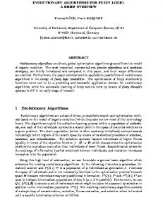
Fig. 1. Abstract representation of the new evolutionary process The introduction of a case-based memory is actually a form of long-term elitism. Elitism forces the EA to maintain the best element of every generation so the current optimum will never be lost. In our case the case-based memory stores these elitists and reintroduces them when the time is right. We believe that this simple approach can improve the exploration capabilities of the EA when convergence has taken place. In Figure 1 the entire process is visualised. At each generational step, the EA tries to optimise the current fitness function. After every attempt one or more individuals of that generation are added to the case-based memory. When a fitness change occurs, the elements of the case-based memory are re-evaluated and one or more of them are reintroduced in the population. There are a number of primary decisions that need to be made. These primary decisions will influence the possibilities of the case-based memory. Especially, they will influence how advanced this memory will be. 1. Which elements will be added to the case-based memory? Currently, the decision was made to present the best element in a generation to the case-based memory. The best individual is added when it does not already exist in the memory. We only store the genotype and fitness information. 2. What kind of structure will we use for the case-based memory? In this paper we simply used a small population as representation for the case-based memory. In later work we will look further at alternative structures. As with the population, the case-based memory size is fixed. We use a strategy called the least recently used strategy (LRU) when removing elements from the case-based memory to add a new individual[SG98]. 3. How will the elements be reintroduced in the population? Again we wanted to use a simple strategy to get a better understanding of the possibilities of the case-based memory. Two simple strategies, random and non-random replacement, will be compared to the standard genetic algorithm with elitism in the experiments. Random replacement just seeds the population with all the elements in the memory, i.e. if k is the number of elements in the memory, then those k elements replace k randomly chosen individuals in the
Raising the Dead
285
Table 2. Main parameters of the evolutionary algorithm. Parameter Value Algorithm type generational GA with elitism Population size 150 Parent selection Fitness proportionate selection Stop condition 1000 generations Mutation type bit-flip mutation Mutation probability 0.1 Crossover type One-point crossover Crossover probability 0.8
population. Non-random replacement removes the worst genotypes from the population and seeds the population with the better elements from the casebased memory. The best element in the memory is determined by evaluating the elements contained in the memory. Next to these primary decisions, there are a number of secondary questions which require an answer. 1. What will the size be of the case-based memory? In order not to slow down the EA process the size of the case-based memory can not be to large. Since the elements also need re-evaluation. We decided to use a case-based memory with a maximum size of 10% of the population size. The maximum size is not always reached during the evolutionary process. 2. When will we add the points to the case-based memory and when will we reintroduce the elements into the population? In the knapsack problem we can easily use the case-based memory every 15 generations since there is a fitness change at those points. But in reality we do not know when the change will take place. So it could be wiser to use the case-based memory every generation. Further, we decided to reintroduce the individuals stored in the case-based memory every time the best fitness drops. This can occur at any point during the evolutionary process and does not have to occur every 15 generations.
5
Experiments
To evaluate the usefulness of the case-based memory we used the periodically changing 0-1 knapsack problem described in Section 3. As explained, we adapted the evaluation function to be able to vary the number of periods and the order of the periods. The EA we used was a standard genetic algorithm with elitism, but again, this could also be some genetic programming or other EA configuration. The goal is to react as fast as possible to an oscillation. We will therefore examine the response time of the population through the performance of the best individual in the population. The response time is measured through the mean % tracking error. A tracking error is a value which measures the difference
286
Jeroen Eggermont et al.
between the optimal fitness and the current best fitness. The entire population does not have to track the changing fitness landscape. Also, when calculating the mean % tracking error over all experiments, the standard deviation is important since a small standard deviation is better than a large one. A very small standard deviation shows that the algorithm is able to track the changing fitness function very closely. In Table 2, the standard parameters for the experiments are described. For each experiments 100 separate runs were performed. For each run, the error resulting from the difference between the best individual in the population and the maximum fitness is collected and these values are used to calculate the mean % tracking error over all 100 runs. These tracking errors and standard deviations can be found in Table 3. In order to compare the tracking errors in a statistically correct way, we removed the trend from the error-data. Since we are only interested in the behaviour of the EA in tracking the changing optimum we calculated the mean % tracking error on the error values of the last 800 generations hence removing the evolutionary trend. Table 3. Resullts for the dynamic 0-1 knapsack problem (example runs for the entries with ∗ are shown in Figure 2, 3 and 4) Periods (= max. weight) {100, 61}∗
Technique
SGA+elitism SGA+Mem(random) SGA+Mem(non-random) {61, 100} SGA+elitism SGA+Mem(random) SGA+Mem(non-random) {100, 61, 30}∗ SGA+elitism SGA+Mem(random) SGA+Mem(non-random) {30, 61, 100} SGA+elitism SGA+Mem(random) SGA+Mem(non-random) {100, 61, 30, 8}∗ SGA+elitism SGA+Mem(random) SGA+Mem(non-random) {8, 30, 61, 100} SGA+elitism SGA+Mem(random) SGA+Mem(non-random)
Mean % track error 3.7018 0.0638 0.0244 2.5523 0.0051 0.0001 9.5358 0.4566 0.0706 17.0504 0.6467 0.5725 30.0398 5.0635 4.0766 36.0144 33.3807 34.1175
Stdev 2.0452 0.2503 0.13 0.9930 0.0504 0.0007 0.7725 0.4598 0.1915 2.8023 0.7169 0.7382 1.27 7.4957 6.2624 2.0562 6.7875 7.7239
From the results in the table it is clear that, by introducing the case-based memory, the tracking capabilities of the standard genetic algorithm are dramatically improved. In order to compare the obtained results for the different EA
Raising the Dead
120
120
periodic fitness changes SGA+elitism
100
100
90
90
periodic fitness changes SGA+Memory(non-random)
Fitness
110
Fitness
110
287
80
80
70
70
60
60
50
0
50
100
150
200 Generations
250
300
350
50
400
0
50
100
150
200 Generations
250
300
350
400
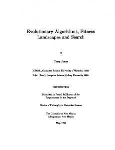
Fig. 2. Example run: Best fitness plot for the 2 periodic 0-1 knapsack problem (left: SGA, right: SGA+Mem(non-random))
120
periodic fitness changes SGA+elitism
110
110
100
100
90
90
80
80
Fitness
Fitness
120
70
70
60
60
50
50
40
40
30
0
50
100
150
200 Generations
250
300
350
30
400
periodic fitness changes SGA+Memory(non-random)
0
50
100
150
200 Generations
250
300
350
400
Fig. 3. Example run: Best fitness plot for the 3 periodic 0-1 knapsack problem (left: SGA, right: SGA+Mem(non-random))
120
periodic fitness changes SGA+elitism
100
100
80
80
Fitness
Fitness
120
60
60
40
40
20
20
0
0
50
100
150
200 Generations
250
300
350
400
periodic fitness changes SGA+Memory(non-random)
0
0
50
100
150
200 Generations
250
300
350
400
Fig. 4. Example run: Best fitness plot for the 4 periodic 0-1 knapsack problem (left: SGA, right: SGA+Mem(non-random))
288
Jeroen Eggermont et al.
configurations we used the student’s t-test [Ros97a]. In Table 4 the results of this statistical test are reported. Table 4. Results Student’s t-test on the data in Table 3 {100, 61} {61, 100} {100, 61, SGA RAN NRA SGA RAN NRAN SGA RAN SGA 0 17.66 17.94 0 25.62 25.7 0 100.9 RAN 17.66 0 1.4 25.62 0 0.98 100.9 0 NRAN 17.94 1.4 0 25.7 0.98 0 118.92 7.75
30} NRAN 118.92 7.75 0
{30, 61, 100} {100, 61, 30, 8} {8, 30, 61, 100} SGA RAN NRAN SGA RAN NRAN SGA RAN NRAN SGA 0 56.71 56.86 0 32.85 40.63 0 3.71 2.37 RAN 56.71 0 0.72 32.85 0 1.01 3.71 0 0.72 NRAN 56.86 0.72 0 40.63 1.01 0 2.37 0.72 0
6
Conclusion and Future Work
Based on all the data we produced from the experiments we can conclude that the introduction of a simple case-based memory in an EA improves the performance of the algorithm in periodically changing environments. As one can see in Table 3 the mean % tracking error of the best individual in the population is much lower when using even this simple case-based memory. To verify whether or not there is a significant difference between the obtained results we performed the students t-test[Ros97a]. In Table 4 the results of this test are shown for every EA combination. From these resuls, we can conclude that the case-based memory approach is significantly better than the simple EA. Also, when examining the standard deviation values we see that the enhanced form of the EA tracks the periodical changes closer that the standard form. When comparing the random and non-random approach, the difference isn’t significant anymore. But, these conclusions are not always true and it seems that the order of the optima is a crucial factor here, as can be seen in Table 3 for the experiment with periods {8, 30, 61, 100}. Also, the standard deviations for the last two experiments are much bigger than that of the standard genetic algorithm. Although we now have information about the possibilities of a simple casebased memory for an EA some extra work has to be done. For instance, we also need to investigate what the influence is of the length between the fitness changes. The length between the fitness changes will determine how converged the population will be when the change occurs. We need to perform experiments on this to know how well our algorithm is able to seed the population with past
Raising the Dead
289
information in order to increase the diversity required for the exploration of an EA. Further, since the size of the case-based memory is limited, it might be possible that, when the length between changes is much larger than the memory, we loose good information. The case-based memory is now only used when a fitness change occurs. It might be useful to use the memory every generation since we do not always know when such a fitness change occurs. Also, the seeding and selection process are very simple strategies. Alternatives to these strategies have to be investigated and compared to the results and performance of the currently used EA configurations. Some work has already been conducted in this area but no real important results have surfaced yet. Further, this simple memory can be extended with a meta-learner which tries to learn which elements are the most suited to seed the population. Such a metalearner could be based on simple regression or some simple machine learning technique. As a result of extending the case-based memory with a meta-learner, we might be able to predict the best seed for future use. As was mentioned in Section 1, next to periodically changing fitness functions there exist non-periodical ones. The case-based memory might also be useful in this context because it seeds the converged population with new information. Important will be how the population will be seeded and which information of the memory will be used. In this case, a meta-learner might come in handy since it would allow us to predict which individual improves the search process. finally we need to incorporate the global case-based memory into other EAs in order to examine the generality of the solution.
Acknowledgement The work presented in this paper was performed at the First COIL Summerschool at the University of Limerick. This summer-school lasted five days. The attendants were divided in groups and were assigned a problem which they had to solve with the techniques discussed in the first days. Our group was assigned the problem of dynamically changing fitness functions. This paper discusses our solution. Through this publication we would like to thank and congratulate the organisers, especially J. Willies and C. Ryan, for their excellent work. To implement the experiments we used the C++ library Evolutionary Objects[Mer,KMS]. Information on how to use the library was given by M. Keijzer who was also our supervisor at the summer-school. We want to thank him for the help and advice he gave us.
References BNKF98. W. Banzhaf, P. Nordin, R.E. Keller, and F.D. Francone. Genetic Programming: an introduction. Morgan Kauffman, 1998. Bra99. J. Branke. Evolutionary approaches to dynamic optimization problems; a survey. GECCO Workshop on Evolutionary Algorithms for Dynamic Optimization Problems, pages 134–137, 1999.
290
Jeroen Eggermont et al.
D. Goldberg. Genetic Algorithms in Search, Optimization and Machine Learning. Addison-Wesley, 1989. GS87. D.E. Goldberg and R.E. Smith. Nonstationary function optimization using genetic algorithms with dominance and diploidy. 2nd International Conference on Genetic Algorithms, pages 59–68, 1987. Hil92. W. Hillis. Co-evolving parasites improve simulated evolution as an opimization procedure. Artificial Life II, pages 313–324, 1992. KMS. M. Keijzer, J.J. Merlo, and M. Schoenauer, editors. Evolutionary Objects. http://sourceforge.net/projects/eodev/. Mer. J.J. Merelo, editor. EO Evolutionary Computation Framework. http://geneura.ugr.es/~jmerelo/EO.html/. Mit97. M. Mitchell. An Introduction to Genetic Algorithms. A Bradford Book, MIT Press, 3th edition, 1997. Par97. J. Paredis. Coevolutionary algorithms. The Handbook of Evolutionary Computation, 1997. Par99. J. Paredis. Coevolution, memory and balance. International Joint Conference on Artificial Intelligence, pages 1212–1217, 1999. Ros97a. W.A. Rosenkrantz. Introduction to Probability and Statistics for Scientists and Engineers. Mc. Graw-Hill, series in Probability and Statistics, 1997. Ros97b. C. Rosin. Coevolutionary Search among Adversaries. PhD thesis, University of California, San Diego, 1997. Rya97. C. Ryan. Diploidy without dominance. 3rd Nordic Workshop on Genetic Algorithms, pages 63–70, 1997. SG98. A. Silberschatz and P. Galvin. Operating System Concepts. Wiley, 5 edition, 1998. SLOA99. L. Spector, W.B. Langdon, U.-M. O’Reilly, and P.J. Angeline, editors. Advances in Genetic Programming, volume 3. MIT Press, 1999. Gol89.