approach is different since we nullify features not just at the training phase but also at the testing phase. Hinton's. arXiv:1610.01239v3 [cs.LG] 7 Oct 2016 ...
Random Feature Nullification for Adversary Resistant Deep Architecture Qinglong Wang1,2 , Wenbo Guo1,3 , Kaixuan Zhang1 , Xinyu Xing1 , C. Lee Giles1 and Xue Liu2
arXiv:1610.01239v3 [cs.LG] 7 Oct 2016
1
College of Information Sciences and Technology, Pennsylvania State University 2 School of Computer Science, McGill University 3 Department of Automation, Shanghai Jiao Tong University
Abstract Deep neural networks (DNN) have been proven to be quite effective in many applications such as image recognition and using software to process security or traffic camera footage, for example to measure traffic flows or spot suspicious activities. Despite the superior performance of DNN in these applications, it has recently been shown that a DNN is susceptible to a particular type of attack that exploits a fundamental flaw in its design. Specifically, an attacker can craft a particular synthetic example, referred to as an adversarial sample, causing the DNN to produce an output behavior chosen by attackers, such as misclassification. Addressing this flaw is critical if a DNN is to be used in critical applications such as those in cybersecurity. Previous work provided various defense mechanisms by either increasing the model nonlinearity or enhancing model complexity. However, after a thorough analysis of the fundamental flaw in the DNN, we discover that the effectiveness of such methods is limited. As such, we propose a new adversary resistant technique that obstructs attackers from constructing impactful adversarial samples by randomly nullifying features within samples. Using the MNIST dataset, we evaluate our proposed technique and empirically show our technique significantly boosts DNN’s robustness against adversarial samples while maintaining high accuracy in classification.
1
Introduction
Deep Neural Networks (DNN) have been recognized for its superior performance in a wide array of areas (Loreggia et al. 2015; Yann and Tang 2016; Bar et al. 2015; Silver et al. 2016; Farabet et al. 2012; Shin, Song, and Moazzezi 2015). However, recent work (Szegedy et al. 2014) uncovered a potential flaw in DNN-powered systems that could be readily exploited by an attacker. Given a DNN model with sufficient details (e.g., hyper-parameters within the model), an attacker can study its weaknesses, examine its class/feature importance, and identify the features that have significant impact on the target’s classification ability. With this knowledge of feature importance, an attacker can minimize the effort in crafting an adversarial sample – a synthetic example generated by modifying a real example slightly in order to make the DNN model believe it belongs to the wrong class with high confidence.
According to a recent study (Goodfellow, Shlens, and Szegedy 2014), the loophole in DNN, which makes it vulnerable to adversarial samples, is that the DNN behaves too much in a linear sense and linear models can be excessively confident when extrapolating an unobserved sample far from the training data. Following this explanation, solutions (Gu and Rigazio 2014; Huang et al. 2015; Miyato et al. 2015) proposed follow the idea of increasing the nonlinearity in DNN. For example, learning with adversarial training is one resistant technique in which a DNN is trained with not only the samples from the original data distribution but also artificially synthesized adversarial ones. It can be shown that such a training strategy is equivalent to increasing the DNN’s nonlinearity by integrating regularization with its objective function. While it has been shown that existing adversary resistant solutions improve DNN’s robustness, they are not completely resistant to adversarial samples. As discussed in Section 5, nonlinearity only makes it harder to craft adversarial samples but does not completely prohibit their effects upon a DNN classifier. In this paper, we show that an adversary can still easily generate adversarial samples from DNN classifiers created from adversarial training. Here, we present a new technique that significantly boosts the DNN’s robustness against adversarial samples. In Section 4 we introduce a random feature nullification in both the training and testing phase, which makes our DNN models non-deterministic. This non-deterministic nature manifests itself when attackers attempt to examine feature/class importance or when a DNN model takes input for classification. As such, there is a much lower probability that attackers could correctly identify critical features for target DNN models. Even if attackers could infer critical features and construct an impactful adversarial sample, the nondeterministic nature introduced at the time when the input is processed will also reduce the effectiveness of adversarial samples. Our random feature nullification approach can also be viewed as dropping neuron units at the input layer. It seems to be a special case of Hinton’s dropout technique (Srivastava et al. 2014) which during training randomly drops units (along with their connections) from a DNN. However, our approach is different since we nullify features not just at the training phase but also at the testing phase. Hinton’s
dropout introduces a non-deterministic nature to DNN during training. Once a training process is completed, a DNN’s model is determined. As such, critical features of the DNN model could still be correctly identified and manipulated to construct synthesized adversarial samples. In Section 5, we compare our random feature nullification to Hinton’s method. As is mentioned above, existing adversary resistant techniques primarily adversarial training). In this work, training DNN with our random feature nullification technique does not change the model linearity, which indicates our technique does not increase complexity of training for a DNN. This orthogonal design principle brings a further benefit. In Section 5, DNN’s robustness can be further boosted by combining our proposed method with existing adversary resistant techniques, particularly adversarial training. The rest of the paper is organized as follows. Section 2 describes the background of adversarial samples. Section 3 surveys relevant work. Section 4 presents our technique and discusses its characteristics. In Section 5, we demonstrate our experiment results where we compare our technique with other learning techniques. Finally, we conclude this work in Section 6.
2
Preliminary
Even though a well trained model is capable of recognizing out-of-sample patterns, a deep neural architecture can be easily fooled by introducing perturbations to the input samples that are often indistinguishable to the human eye (Szegedy et al. 2014). These so-called “blind spots”, or adversarial samples, exist because the input space of DNN is unbounded (Goodfellow, Shlens, and Szegedy 2014). Based on this fundamental flaw, we can uncover specific data samples in the input space able to bypass DNN models. More specifically, it was studied in (Goodfellow, Shlens, and Szegedy 2014) that attackers can find the most powerful blind spots via effective optimization procedures. In multiclass classification tasks, such adversarial samples can cause a DNN model to classify a data point into a random class besides the correct one (sometimes not even a reasonable alternative). Furthermore, according to (Szegedy et al. 2014), DNN models that share the same design goal, for example recognizing the same image set, all approximate a common highly complex, nonlinear function. Therefore, a relatively large fraction of adversarial examples generated from one trained DNN will be misclassified by the other DNN models trained from the same data set but with different hyper-parameters. Therefore, given a target DNN, we refer to adversarial samples that are generated from other different DNN models but still maintain their attack efficacy against the target as crossmodel adversarial samples. Adversarial samples are generated by computing the derivative of the cost function with respect to the network’s input variables. The gradient of any input sample represents a direction vector in the high dimensional input space. Along this direction, an small change of this input sample will cause a DNN to generate a completely different prediction result. This particular direction is important since
it represents the most effective way of degrading the performance of a DNN. Discovering this particular direction is realized by passing the layer gradients from output layer to input layer via back-propagation. The gradient at the input may then be applied to the input samples to craft an adversarial examples. To be more specific, let us define a cost function L(θ, X, Y ), where θ, X and Y denotes the parameters of the DNN, the input dataset, and the corresponding labels respectively. In general, adversarial samples can be crafted by adding to real ones via an adversarial perturbation δX. In (Goodfellow, Shlens, and Szegedy 2014), the efficient and straightforward fast gradient sign method was proposed for calculating adversarial perturbation as shown in (1): δX = φ · sign(JL (X)),
(1)
here δX is calculated by multiplying the sign of the gradients of real sample X with some coefficient φ. JL (X) denotes the derivative of the cost function L(·) with respect to X. φ controls the scale of the gradients to be added. Adversarial perturbation indicates the actual direction vector to be added to real samples. This vector drives real sample X towards a direction that the cost function L(·) is significantly sensitive to. However, it should be noted that δX must be maintained within a small scale. Otherwise adding δX will cause significant distortions to real samples, leaving the manipulation to be easily detected.
3
Related Work
To counteract adversarial samples, recent research mainly focuses on two lines of techniques – adversarial training and model complexity enhancement. In this section, we summarize these techniques and discuss their limitations as follows. Adversarial training approaches usually augment the training set by integrating adversarial samples (Szegedy et al. 2014). More formally, this data augmentation approach can be theoretically interpreted as adding regularization to the objective function of DNN. This regularization is designed to penalize certain gradients obtained by deriving the objective function with respect to the input variables. The penalized gradients indicate a direction in the input space that the objective function is the most sensitive. For example, recent work(Goodfellow, Shlens, and Szegedy 2014) introduces a novel objective function. This new objective function directly combines a regularization term with the original cost function. In this way, the DNN is enhanced to handle the worst case scenario. Instead of training DNN with a mixture of adversarial and real samples, other work (Nøkland 2015) uses only adversarial samples. Despite the difference between these strategies, a unifying framework, DataGrad (Ororbia II, Giles, and Kifer 2016), generalizes deep adversarial training and helps explain prior approaches (Gu and Rigazio 2014; Rifai et al. 2011). However, since adversarial training still falls into the category of data augmentation, it does not train DNN with the complete data set. In other words, adversarial training is still vulnerable to the adversarial samples not foreseen.
Model complexity enhancement is another approach recently proposed to improve the robustness of DNN. Recent work (Papernot et al. 2016a), denoted as distillation enhances a DNN model by enabling it to utilize other informative input. More specifically, for each input training sample, instead of using its original hard label which only indicates whether it belongs to a particular class, the enhanced DNN utilizes a soft label, which means there is a probability of belonging to every available class. In order to use this more informative soft label, two DNN must be designed successively and then stacked together. One DNN is designed for generating more informative input samples. Then, the other DNN is trained with these more informative samples in the standard way. However, once the architecture of distillation is disclosed to attackers, it is always possible to find adversarial samples based on the stacked model of distillation and DNN. More specifically, if an attacker (Carlini and Wagner 2016) generates adversarial samples by artificially reducing the magnitude of input to the final softmax function and modifies the objective function used for generating adversarial samples (Papernot et al. 2016b), the defensively distilled networks can be attacked. A de-noising autoencoder (Gu and Rigazio 2014) is proposed to filter out adversarial perturbations. However, it suffers the same problem (Papernot et al. 2016a). To be more specific, once the architecture of stacked DNN and auto-encoder is disclosed, attackers can generate adversarial samples by treating it as a normal feed-forward DNN only with more hidden layers. Indeed, adversarial samples of this stacked DNN (Gu and Rigazio 2014) show even smaller distortion compared with adversarial samples generated from the original DNN. Thus, a successful method for increasing model complexity requires the property that even if the model architecture is disclosed, it is impossible to generate adversarial samples based on it. According to the analysis above, neither adversarial training nor model complexity enhancement is sufficient for defending against adversarial samples. Therefore, we propose a new technique to build an adversary resistant DNN architecture which is not only robust against adversarial samples, but also robust against the mechanism of generating unseen adversarial samples specific to our proposed architecture.
4
Random Feature Nullification
Figure 1 illustrates a DNN using our random feature nullification method. Different from the most standard DNN, it introduces an additional layer between the input and the first hidden layer. The additional hidden layer is a nondeterministic layer playing the role of introducing randomness at both the training and testing phases. In particular, it randomly nullifies the features within the input. Consider image recognition as an example. When a DNN passes an image sample through the layer, it randomly nullifies some pixels within the image and then feeds the partial nullified image to the first hidden layer. The proportion of pixels nullified is determined from the parameter p. Next, we describe the DNN model with random feature nullification followed by the description on how to train such a model. Then, we explain why it is resistant to adversarial samples. Finally, we
f(X, Ip)
.
Input X
Feature Nullification Ip Hidden Layer
Hidden Layer
Output Layer
...
Figure 1: An example DNN that adopts our random feature nullification method. analyze the random feature nullification method and compare it with other adversary resistant techniques.
4.1
Model Description
Given an input sample denoted by X ∈ RN ×M , random feature nullification amounts to performing elementby-element multiplication of X and Ip . Here, Ip is a mask matrix sharing the same dimensionality with X (i.e., Ip ∈ RN ×M ). Each element in Ip is an independent, identically distributed (i.i.d.) random variable following Bernoulli distribution B(1, p) with the same value in p. In this work, an element in Ip takes the value 0 with probability of p and value 1 with probability of 1 − p. From Figure 1, random feature nullification can be viewed as a process in which the layer performing random feature nullification simply passes nullified features through to a standard DNN. Therefore, we have the following objective function: � min L θ, f (X, Ip ), Y . (2) θ Here, Y and θ are respectively the label of input X as well as the coefficient parameters that need to be learned during training. Function f (X, Ip ) represents a random feature nullification operation that has the form of f (X, Ip ) = X Ip . In this form, denotes the Hadamard-Product. The DNN in Figure 1 can be trained using stochastic gradient descent in a manner similar to a standard DNN. The only difference is that for each training sample we randomly take a value for Ip based on p. During forward and backward propagation for that training sample, we hold onto the value of Ip until the arrival of the next training sample. In�this way, we can compute the derivative of L θ, f (X, Ip ), Y with respect to θ and update θ accordingly.
4.2
Adversary Resistant Analysis
To craft an adversarial sample, recall that an attacker needs to produce an adversarial perturbation and then add it to a real sample. As is shown in Equation 1, the adversarial perturbation is produced by computing the derivative of a
Feed-forward DNN Backpropagation
Feed-forward DNN
ial sample that the attacker would use to fool the blackbox. Taking as input the synthesized adversarial sample, the blackbox performs random feature nullification and then feeds the nullified adversarial sample to the DNN in the blackbox. This nullified adversarial sample can be denoted by � � X + δX Ip∗ Ip = X Ip + δ Ip∗ Ip . (4) Here, X Ip is a nullified real sample, and δ Ip∗ Ip represents the adversarial perturbation added to it. As is mentioned above, δX is the most impactful adversarial perturbation to the DNN in the blackbox. With that multiplying a matrix represented by Ip∗ Ip , the impactful adversarial perturbation is distorted and no longer effective in making the DNN misclassified. To validate this empirically, we conduct experiments and show the result in Section 5.
4.3
Figure 2: A running example of generating an adversarial sample and testing it on the DNN with random feature nullification. DNN’s objective function. Following this process, an at-� ˜ Ip ), Y tacker can take the partial derivative of L θ, f (X, ˜ with regard to X. From the chain rule, this can be described as � ˜ Ip ), Y ∂L θ, f ( X, ˜ = JL (X) ˜ ∂X (3) ˜ Ip ) ∂f (X, . = JL (f ) · ˜ ∂X � ˜ p ),Y ∂L θ,f (X,I ˜ represents a where JL (f ) = . Note that X ˜ p) ∂f (X,I real sample and an adversarial sample can be produced by ˜ to X. ˜ adding φ · sign(JL (X)) In Equation (3), JL (f ) can be easily computed. How˜ p) ∂f (X,I ˜ ∂X
ever, contains random variable Ip , making derivative computation impossible. In other words, random variable Ip prohibits attackers from computing a derivative for producing an adversarial perturbation. With this randomness, the only way to generate an ‘adversarial sample’ for an attacker is to draw a sample from Ip and then replace random variable Ip with that sample. However, even if an attacker draws a sample that plays the optimal substitution for random variable Ip , an adversarial sample still cannot be sufficiently impactful. We theoretically test this hypothesis as follows. Assume an attacker draws a sample, Ip∗ representing the optimal substitution for Ip . Using this sample, the attacker computes an adversarial perturbation denoted by δX Ip∗ for real sample X. As is shown in Figure 2, we take as a blackbox the DNN with random feature nullification. δX represents the most impactful adversarial perturbation to the DNN in the blackbox, and δX Ip∗ is a synthesized adversar-
Comparison
In this work, we introduce randomness to a DNN, making it robust to adversarial samples. As is discussed in Section 3, there are other adversary resistant techniques. Here, we analyze why those resistant techniques fail to counteract adversarial samples, especially when attackers craft adversarial samples based on the model enhanced by these techniques. According to a recent study (Ororbia II, Giles, and Kifer 2016; Kang, Li, and Tao 2016; Wager, Wang, and Liang 2013), most adversary resistant techniques are actually instances of optimizing a general, regularized objective. In other words, they can be viewed as imposing regularization to DNNs (see the equation below). min G(θ, X, Y ) = L(θ, X, Y ) + γ · R(θ, X, Y ), θ
(5)
where L(θ, X, Y ) is an objective function of a standard DNN, and R(θ, X, Y ) is a regularization term. Here, γ controls the strength of the regularization term. To craft an adversarial sample, an attacker can easily produce an adversarial perturbation by computing derivative with regard to a real sample as follows ∂G(θ, X, Y ) ∂X � (6) ∂ L(θ, X, Y ) + γR(θ, X, Y ) = . ∂X With the regularization term, which penalizes the direction most effective in crafting adversarial sample, prior studies indicate that adding φ · sign(JG (X)) to sample X becomes less effective in fooling the corresponding DNN model. However, as we will show in Section 5, an attacker can still make a DNN misclassified by simply increasing scale factor φ because regularization only imposes limited penalty to the direction most impactful for producing adversarial perturbations. In a recent study (Goodfellow, Shlens, and Szegedy 2014), Goodfellow et al. explain this as a problem of exploring an unbounded adversarial sample space because adversarial samples occur in an unbounded subspace and adversarial training is a data augmentation technique which is never able to improve DNN’s robustness with all adversarial samples. Our random feature nullification method can be JG (X) =
also viewed as a way to penalize the direction most impactful for producing adversarial perturbations. Different from adversarial training, the penalty is imposed by a matrix (see Equation 4). Therefore, it can impose penalty to all adversarial samples and provide strong resiliency to DNNs. In Section 5, we show our random feature nullification method significantly advance adversarial training.
5
Evaluation
Here, we first evaluate our proposed technique (i.e., random feature nullification) against adversarial training, a traditional solution proved to be effective in undermining the impact of adversarial samples. We also empirically compared our random feature nullification method against Hinton’s dropout to showcase the differences. Last but not least, we integrate our solution along with adversarial training and evaluate its performance against standalone solutions – random feature nullification and adversarial training respectively.
5.1
Experimental Design and Setup
There are two outcome metrics that we focus on in our evaluation – model resiliency and classification accuracy. We deem a solution superior if we observe higher robustness against adversarial samples while incurring no or only negligible degradation in classification accuracy. Our evaluation data comes from the publicly available MNIST dataset comprised of 60,000 training samples and 10,000 testing samples. To evaluate classification accuracy, we use the 10,000 cases as they are across all aforementioned methods. For model resiliency evaluations, we need to construct method-specific adversarial samples based on the 10,000 hold out cases. We assumed attackers had acquired the full knowledge of each DNN model (i.e. hyper-parameters) and could construct most ‘impactful’ adversarial samples to their best knowledge, which gives them competitive advantage over our defense systems. Therefore, the observed resiliency should reflect the lower bound of model robustness against adversarial samples. To identify the optimal nullification rate in our proposed method for MNIST data, we randomly nullify features with various proportions – from 10% to 70% at 10% increment – at both training and testing phrases. We then evaluate the corresponding classification accuracy and model resiliency. As is shown in Table 1, we achieved the maximum resiliency against adversarial samples at 50% nullification rate. Classification accuracy wise, our proposed solution demonstrates roughly consistent performance at different nullification rates. Based on this result, we adopted 50% as our feature nullification rate in this evaluation.
5.2
Experimental Results
We implement five distinct DNN models by training them with different learning techniques specified in Table 2. We present the architecture of these DNN models as well as the corresponding hyper-parameters in Appendix. In Table 2, we also show the classification accuracy and model
Nullification rate
Classification error rate Accuracy
Resiliency
10%
0.0135
0.4130
20%
0.0133
0.3883
30%
0.0138
0.2891
40%
0.0149
0.2305
50%
0.0170
0.2154
60%
0.0209
0.2323
70%
0.0266
0.2366
Table 1: Classification accuracy vs. model resiliency with various feature nullification rates. resiliency of these DNN models against various coefficients φ. As is described in Section 2, coefficient φ represents the scale of the perturbation added to a real sample. As a result, Table 2 also illustrates a few adversarial samples (i.e., image samples distorted based on the scale of perturbation). With a subtle perturbation added to samples, Table 2 first shows that the standard DNN model exhibits a high classification error rate when classifying adversarial samples. This indicates weak model resiliency to adversarial samples. Following Hinton’s dropout and adversarial training respectively, we retrain the model and discover that the two DNN models newly trained present a certain level of improvement in model resiliency. The reason is that both learning techniques provide DNNs with an additional regularization benefit. The regularization increases the nonlinearity to the model, making it resistant to adversarial samples. Since adversarial training can provide regularization benefit beyond that provided by using dropout, Table 2 also shows the DNN model derived from adversarial training advances that from Hinton’s dropout in terms of model robustness to adversarial samples. In Table 2, we also discover both adversarial training and Hinton’s dropout only increase the difficulty for attackers in crafting adversarial samples. With the increase in coefficient φ, adversarial samples (handwritten digits in Table 2) are further distorted and model resiliency is attenuated. According to a prior study in (Goodfellow, Shlens, and Szegedy 2014), this is due to the fact that adversarial samples occur in unbounded subspaces, and regularization strategies cannot penalize all directions effectively in generating adversarial samples. Compared with the aforementioned methods using regularization for model robustness improvement, our random feature nullification exhibits a significant reduction in a model’s vulnerability to adversarial samples. As is shown in Table 2, a DNN model trained with random feature nullification demonstrates a low error rate when classifying adversarial samples. In addition, we observe that the model resiliency still remains relatively strong even though a harsh perceptible perturbation is added to samples (i.e., φ = 0.35). One intuitive explanation behind this observation is that our
Classification error rate Learning technique
Resiliency (Different step)
Accuracy φ = 0.15
φ = 0.25
φ = 0.35
Standard
0.0207
0.9181
0.9944
0.9999
Hinton’s dropout
0.0202
0.8049
0.9614
0.9904
Adversarial Training
0.0201
0.3229
0.7263
0.9238
bined technique also advances our random feature nullification technique significantly. This is due to the fact that random feature nullification and adversarial training penalize adversarial samples in two different manners, and a combination of the two amplifies the model resiliency that each technique can demonstrate. Last but not least, Table 2 also shows that neither our proposed technique nor the aforementioned combined technique brings about degradation in classification accuracy. Compared with the standard DNN model as well as the other two models trained with regularization strategies, models with random feature nullification exhibit high accuracy in classification. This is due to the fact that feature nullification makes data samples less informative and we enlarge the training dataset for compensating such information loss.
6
Random feature nullification
0.0148
0.2154
0.4764
0.6615
Random feature nullification & adversarial training
0.0149
0.0620
0.1543
0.3486
Table 2: Classification accuracy and model resiliency across five distinct models derived from (1) standard method, (2) Hinton’s dropout, (3) adversarial training, (4) random feature nullification and (5) the combination of adversarial training and random feature nullification. For training a DNN model with Hinton’s dropout, the probability of dropping units is set at 0.25.
proposed technique randomly knocks down a group of features which contain some features with high impacts upon fooling a DNN model. Recall that random feature nullification imposes randomness to samples. Applied to image recognition, this technique can be viewed as a way of image preprocessing in which our technique randomly nullifies a certain proportion of pixels within an image before passing it to a DNN. As such, it can be combined with other adversary resistant techniques. We expect such a combination can further improve model robustness. To validate this, we combine our random feature nullification technique with adversarial training and compare it with standalone solutions discussed above. Table 2 specifies the classification accuracy and model resiliency of the combined technique. Compared with standalone adversarial training, our random feature nullification exhibits superior performance with regard to counteracting adversarial samples. In addition, we observe that the com-
Conclusion
We proposed a new technique for constructing DNN models that are robust to adversarial samples. Our design is based on a thorough analysis of both the fundamental flaw of DNNs and the limitations of current solutions. Using our proposed technique, we show it is impossible for an attacker to craft an impactful adversarial sample that can force a DNN to provide adversary-selected output. This implies that our proposed technique no longer suffers from attacks that rely on generating model-specific adversarial samples. For comparison, we demonstrated that recently studied adversarial training methods are not sufficient for defending against adversarial samples. Applying our new technique on the MNIST data set, we empirically demonstrate that our new technique significantly reduces the error rates in classifying adversarial samples. Furthermore, our new technique does not impact DNN’s performance in classifying legitimate samples. Future work will entail investigating the performance of our technique for a wider variety of applications.
7
Appendix
To augment the experimental setup presented in Section 5, the following table indicates the hyper parameters that we used for model training.
References [Bar et al. 2015] Bar, Y.; Diamant, I.; Wolf, L.; and Greenspan, H. 2015. Deep learning with non-medical training used for chest pathology identification. In SPIE Medical Imaging, 94140V–94140V. International Society for Optics and Photonics. [Carlini and Wagner 2016] Carlini, N., and Wagner, D. 2016. Defensive distillation is not robust to adversarial examples. arXiv preprint arXiv:1607.04311. [Farabet et al. 2012] Farabet, C.; Couprie, C.; Najman, L.; and LeCun, Y. 2012. Scene parsing with multiscale feature learning, purity trees, and optimal covers. arXiv preprint arXiv:1202.2160. [Goodfellow, Shlens, and Szegedy 2014] Goodfellow, I. J.; Shlens, J.; and Szegedy, C. 2014. Explaining and harnessing adversarial examples. arXiv preprint arXiv:1412.6572.
Learning technique
Hyper Parameters Network Structure
Activation Func.
Learning rate
Batch size
Epoch
Standard
784-100-100-10
Tanh
0.1
100
100
Hinton’s Dropout
784-100-100-10
Tanh
0.1
100
100
Adv. training
784-100-100-100-10
Tanh
1
100
100
RFN
784-100-100-10
Sigmoid
0.1
1000
100
RFN & Adv. training
784-100-100-10
Tanh
0.1
1000
100
Table 3: The Hyper parameters for model training. Note that the network structure specifies the number of hidden layers and hidden units in each layer. For example, 784-100-10010 indicates a DNN with 4 hidden layers, and the numbers of hidden units across each layer are 784, 100, 100 and 10, respectively. For Hinton’s dropout, we set the dropout rate at 25%. [Gu and Rigazio 2014] Gu, S., and Rigazio, L. 2014. Towards deep neural network architectures robust to adversarial examples. arXiv preprint arXiv:1412.5068. [Huang et al. 2015] Huang, R.; Xu, B.; Schuurmans, D.; and Szepesv´ari, C. 2015. Learning with a strong adversary. CoRR, abs/1511.03034. [Kang, Li, and Tao 2016] Kang, G.; Li, J.; and Tao, D. 2016. Shakeout: A new regularized deep neural network training scheme. In AAAI Conference on Artificial Intelligence. [Loreggia et al. 2015] Loreggia, A.; Malitsky, Y.; Samulowitz, H.; and Saraswat, V. 2015. Deep learning for algorithm portfolios. In AAAI Conference on Artificial Intelligence. [Miyato et al. 2015] Miyato, T.; Maeda, S.-i.; Koyama, M.; Nakae, K.; and Ishii, S. 2015. Distributional smoothing with virtual adversarial training. stat 1050:25. [Nøkland 2015] Nøkland, A. 2015. Improving back-propagation by adding an adversarial gradient. arXiv:1510.04189 [cs]. [Ororbia II, Giles, and Kifer 2016] Ororbia II, A. G.; Giles, C. L.; and Kifer, D. 2016. Unifying adversarial training algorithms with flexible deep data gradient regularization. arXiv:1601.07213 [cs]. [Papernot et al. 2016a] Papernot, N.; McDaniel, P.; Wu, X.; Jha, S.; and Swami, A. 2016a. Distillation as a defense to adversarial perturbations against deep neural networks. In 2016 IEEE Symposium on Security and Privacy (SP), 582– 597. [Papernot et al. 2016b] Papernot, N.; McDaniel, P.; Jha, S.; Fredrikson, M.; Celik, Z. B.; and Swami, A. 2016b. The limitations of deep learning in adversarial settings. In 2016 IEEE European Symposium on Security and Privacy (EuroS&P), 372–387. IEEE.
[Rifai et al. 2011] Rifai, S.; Vincent, P.; Muller, X.; Glorot, X.; and Bengio, Y. 2011. Contractive auto-encoders: Explicit invariance during feature extraction. In Proceedings of the 28th international conference on machine learning (ICML-11), 833–840. [Shin, Song, and Moazzezi 2015] Shin, E. C. R.; Song, D.; and Moazzezi, R. 2015. Recognizing functions in binaries with neural networks. In 24th USENIX Security Symposium (USENIX Security 15), 611–626. [Silver et al. 2016] Silver, D.; Huang, A.; Maddison, C. J.; Guez, A.; Sifre, L.; Van Den Driessche, G.; Schrittwieser, J.; Antonoglou, I.; Panneershelvam, V.; Lanctot, M.; et al. 2016. Mastering the game of go with deep neural networks and tree search. Nature 529(7587):484–489. [Srivastava et al. 2014] Srivastava, N.; Hinton, G. E.; Krizhevsky, A.; Sutskever, I.; and Salakhutdinov, R. 2014. Dropout: a simple way to prevent neural networks from overfitting. Journal of Machine Learning Research 15(1):1929–1958. [Szegedy et al. 2014] Szegedy, C.; Zaremba, W.; Sutskever, I.; Bruna, J.; Erhan, D.; Goodfellow, I.; and Fergus, R. 2014. Intriguing properties of neural networks. In International Conference on Learning Representations. [Wager, Wang, and Liang 2013] Wager, S.; Wang, S.; and Liang, P. S. 2013. Dropout training as adaptive regularization. In Burges, C. J. C.; Bottou, L.; Welling, M.; Ghahramani, Z.; and Weinberger, K. Q., eds., Advances in Neural Information Processing Systems 26. Curran Associates, Inc. 351–359. [Yann and Tang 2016] Yann, M. L.-J., and Tang, Y. 2016. Learning deep convolutional neural networks for x-ray protein crystallization image analysis. In AAAI Conference on Artificial Intelligence.