TH E B ALANCING EFFECT IN B RAIN-M ACH INE INTERACT IO N FOTINI PALLIKARI Solid State Physics Department, Faculty of Physics, National and Kapodistrian University of Athens, Greece email:
[email protected]
Abstract. The meta-analysis of Intangible Brain-Machine Interaction (IMMI) data with random number generators (RNG’s) (Bösch, 2006) is re-evaluated through the application of rigorous and recognised mathematical tools. The current analysis shows that the statistical average of the true RNG-IMMI data is not shifted from chance by direct mental intervention, thus refuting the IMMI hypothesis. A facet of this general statistical behavior of true RNG-IMMI data is the statistical balancing of scores observed in IMMI tests where binary testing conditions are adopted. The actual dynamics that had been supporting the elusive IMMI effect are shown to be related to the psychology of experimenters. The implications of the refutation of the IMMI hypothesis especially on associated phenomena are also discussed.
Keywords Meta-analysis; Psychology; random number generators; funnel plot; Markovian process.
INTRODUCTION The IMMI hypothesis states that “the statistical average of random numbers is shifted away from the theoretically expected value by mental effort alone”. The difference between the observed statistical average from many IMMI tests and the expected statistical average is called the “mean-shift”. According to the IMMI hypothesis the value of this mean-shift should be found significantly above zero. In other words, the hypothesis predicts that just by applying our intention, our wish or desire, we can introduce some modulation in the statistical outcomes of a random process, without the mediation of a mind-machine interface device. Such mind-machine interface devices exist to date and are used for instance to drive the mechanical parts of neuroptosthetics (Medina, 2012 & Serruya, 2002).
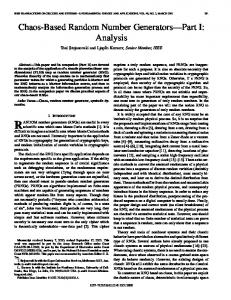
Twenty five years ago I started investigating the controversial world of the Intangible Brain-Machine Interaction (IMMI). It was during my sabbatical from the University of Athens, under the last of the series of Perrott-Warrick scholarships that brought me to Cambridge, UK. The scholarship supported my visit to the Mind Science Foundation (MSF) in San Antonio, Texas in 1991 where I was introduced to Dr Helmut Schmidt and his electronic random number generators (Schmidt, 1976 & 1987). These were interesting looking black boxes with buttons and switches featuring a linear or circular array of LED lights flashing randomly according to several modes of operation, figure 1. On one of its modes of operation, the linear array of lights of my IMMI device was set to flash either in one or the opposite direction. Our task was to mentally influence the progression of flashing lights in the specific direction of our choice, simply by thinking and wishing for it to happen. At the end of a run the digital display placed at its front showed a number which indicated the degree of success of our efforts. Dr Schmidt lent me one of his electronic IMMI devices so that I could assist his data collection as part of his IMMI experiment with prerecorded targets (Schmidt et al, 1993) and also that I could additionally familiarize with it. So, I began testing the IMMI hypothesis.
The present work will review the evidence in favour and against the IMMI hypothesis with true random number generators (RNG’s) involving the author’s own experimental observations and data treatment during the last 25 years. Yet, the major part of the analysis will involve the totality of data published during the last 35 years by independent experimenters and presented in the (Bösch et al, 2006) meta-analysis.
THE BALANCING EFFECT IN IMMI TESTS The adopted protocol of testing the IMMI hypothesis with the Schmidt RNG machine, consisted of one “run” of ten trials, while attempting to mentally influence the random progression of LED lights followed by another ten trials, under the same mode of operation, while allowing the machine to operate without consciously trying to mentally affect its statistics. The former type of data was named “intention” and the latter were the “no intention” data.
how many standard errors is the average of collected numbers shifted away from the chance score. Yet, the plot of cumulative z-scores against the number of data revealed an additional intriguing element: The cumulative scores of the “intention” condition were in the direction of intention, balancing about zero mean-shift the cumulative scores of the no-intention condition. The scores were even reaching a statistically significant level in both directions, figure 2a. The data shown on the top graph of figure 2a are the intention data exhibiting positive values of the cumulative z-scores (i.e. in the direction of intention) exactly as the IMMI hypothesis
At a certain point there were close to 1000 trials collected, that is, about 1000 random numbers presented as z-scores in each of the two testing conditions. That made a relatively small size of a study. The z-score evaluates by
1
statistical balancing of scores in a number of tests (Pallikari-Viras, 1997), figures 2b to 2d. The size of these tests was much smaller, about 250 to 500 of collected numbers in each one of them. In one of these tests, the cumulative z-scores of both conditions were observed to remain positive and not even exceeding chance levels, figure 2b. In another IMMI test a cross-over was observed around about 100 collected data. At that point of crossover, the intention data from positive assumed negative values while the opposite was observed for the nointention data, figure 2c. Again here the overall mean shift was not statistically different from zero. Finally, in a fourth test a similar cross-over as in the case of figure 2c was observed around about 50 collected data in each condition leaving the overall cumulative z-score again not statistically different from zero, figure 2d.
(a)
Prior to the observation of the statistical balancing effect, observations of similar result were independently reported. One of such cases was the “decline effect” (Rhine, 1969; Rhine 1971). The phenomenon appeared as a tendency to score below chance around the middle of a long run to render the overall score to chance and erase the previous scoring-above-chance success. Another similar report referred to the “differential effect”. According to that in IMMI experiments when people are asked to produce an effect under two different conditions, they tend to score above chance in the one of them and below chance in the other (Rao, 1965). The net score would thus be a zero mean-shift. In addition, a statistical balancing of scores was also observed within the large database of Princeton Engineering Anomalies Research (PEAR) (Jahn et al, 1987). On page 119 of the book “Margins of Reality-The Role of Consciousness in the Physical World” it reads: “When all intention data were merged with no-intention data, they yielded the theoretically expected Gaussian curve, i.e. no meanshift.” There were also at least, to the best of our knowledge, two reports of the Balancing Effect published by (Bierman et al, 1994 & Houtkooper, 2002) not prior, but this time following its first publication in related research literature.
(b) Fig. 1. Two electronic IMMI-RNG machines manufactured by Dr H. Schmidt. (a) The borrowed RNG with which the first IMMI tests were performed, through which the Balancing Effect was first observed. Its orthogonal parallelepiped shape features 31 LED lamps on its top and a digital display of the scores in the front. (b) This model of RNG device features 9 LED lamps placed circularly in front and a digital display. It was purchased by the author in 1995.
predicts. The bottom data in figure 2a are the no-intention data, surprisingly keeping negative values of the cumulative z-scores (i.e. against the direction of intention) balancing the scores of the intention condition. Around about 200-250 of collected data, the cumulative z-scores appear to reach statistically significant levels: i.e. +2,5 and -3,0. The experience during these tests was imposing the impression that the mind could command the progression of lights.
All those independently reported cases were describing the same behavior of statistical balancing observed in various related databases, that is: When a large enough number of random data is collected under psi or non-psi oriented conditions as part of a IMMI experiment, the overall score of the database will exhibit a zero meanshift from chance.
The end result of such balancing of scores was, of course, that the overall statistical average of numbers collected both under intention and no-intention conditions was not shifted away from chance, indicated in figure 2a-d by the dotted line at z=0. This bizarre statistical behavior of the random numbers generated by the Schmidt electronic RNG-IMMI machine was termed “the balancing effect” and presented at the 36th PA convention in Toronto, Canada in 1993 (Pallikari-Viras, 1998).
The first observation of the Balancing Effect, figure 2a, was simply a facet of the same fundamental law underlying all these diverse observations, i.e. the law of large numbers, that can manifest itself in more than one way in very large studies as well as in smaller datasets. According to the law of large numbers the average of the outcomes obtained from a large number of IMMI trials with RNG’s gets closer to the expected value, i.e. close to chance, as more trials are collected.
Further testing of the IMMI hypothesis (the first RNG machine had meanwhile returned back to Dr Schmidt, its chips were replaced by new ones and it was then returned to me for the follow-up studies) failed to observe the same
2
Z Values
(b)
(a)
(c)
(d) Number of data
Fig. 2. Cumulative z-scores vs the number of data, N, in four MicroPK tests with an electronic Schmidt RNG (PallikariViras, 1997 & 1998). (a) Scores exhibit the balancing effect: Intention data are positive reaching statistically significant levels and no-intention data are negative also reaching statistically significant levels; N is close to 1,000. (b) to (d): The data do not exhibit the previous statistical balancing, yet they always maintain an overall zero mean-shift. The size N in (b) and (c) is about 250 and about 500 in (d).
To support the statistical balancing observation in IMMI tests with true RNG’s came a sequence of events. First, a three-leg consortium of research groups at Freiburg, Giessen, and Princeton (IMMI PortREG) was formed in 1996 to replicate prior evidence indicating that the mind could affect the random statistical behavior of electronic random number generators (Jahn et al, 1987). This large experiment failed, however, to replicate the IMMI hypothesis; the overall statistical average was found to be within chance in each one of the three experimental groups of this consortium (Jahn et al, 2000). Finally, a meta-analysis of all true RNG-IMMI data was performed triggered by this large replication failure (Bösch, 2006). Can observations that disprove the IMMI hypothesis apply not to just a part of IMMI tests, but to the large
database of all IMMI tests that have ever been published? If the answer is “yes”, then why do IMMI test scores exist which significantly deviate from chance? To answer adequately questions like the above the existing IMMI evidence has been subjected to a variety of data analyses: a) the Rescaled Range Analysis which reveals the presence of long-range correlations in time series; b) the graphical representation of the RNG data on funnel plots, clearly revealing that the IMMI hypothesis is refuted while indicating the presence of correlations in the database; and c) the Markovian representation of IMMI true RNG bits which can adequately replicate the IMMI funnel plot, making itself a suitable candidate of the mechanism that introduces correlations in the database.
3
Fig. 3. Funnel plot of scores, pi, reported in IMMI data meta-analysis with true RNG’s (Bösch et al, 2006). Blue dashed curves: The statistical border that should theoretically envelope the 95% of random plotted data. Red solid curves: The broadened new position of the blue dash lines that adequately envelopes the 95% of plotted data. Dashed vertical line: Indicates the position of the most representative effect size. Dash-dotted vertical line: Indicates the position of the simple statistical average of all IMMI effect sizes, ℘ = 0,51; standard error=0,002. The standard errors of pi values are not displayed on the graph for clarity. This graph was published in (Pallikari, 2015).
DATA ANALYSIS AND MODELLING The Rescale Range Analysis. The part of IMMI records generated at the IGPP Institute, the FAMMI (Freiburg Anomalous Mind Machine Interaction) during the three-leg IMMI consortium, was subjected to the Rescaled Range Analysis, or R/S analysis (Pallikari, 1998; Bauer, 1998). The aim of the analysis was to identify whether the IMMI records of tests arranged in time series were adequately random or correlated (Pallikari et al, 1999; Pallikari et al, 2000; Pallikari, 2001; Pallikari, 2002).
correlations or by antipersistent correlations, but an overall persistence typically marks natural phenomena (Pallikari et al, 1999). The natural records may tend to persistently deviate away, either above or below chance, while the Hurst exponent ranges as: 0,5 > ≥ 1. In the case of anti-persistence, the variation of natural records keep close to, without deviating away from, chance as compared to the random case. The Hurst exponent is found then to range as: 0 ≤ < 0,5. In absence of correlations in a time series of natural records, the Hurst exponent is = 0.5.
The R/S analysis estimates a parameter, the Hurst exponent, indicated by H. The records of natural phenomena are usually correlated; either by persistent
Experimental Control Calibration
There were three types of FAMMI-IMMI data that were
H 0.521 0.508 0.505
SE 0.004 0.003 0.006
N 450,000 450,000 500,000
Table 1. Hurst exponents, H, of IMMI data estimated by the R/S analysis. N: size of study; SE: standard error of H.
4
subjected to the R/S analysis; the experimental, the control and the calibration data. The “experimental data” were the records of many individual IMMI experimental sessions where operators were trying to mentally influence the behavior of the RNG device. These segments of individual tests were later merged together into the large “experimental” data time series.
dependent upon the associated standard error. More precisely, IMMI experiments with very fast RNG’s allow for the collection of a very large number of data. The size of experiments shown in table 1 ranges from 450 to 500 thousands of numbers. For such very large data sets the associated standard errors (se) are very low, since they are estimated as the ratio of the population standard deviation divided by the square root of the size of data. Standard error can therefore be as small as 10-3, table 1. Larger experimental sizes yield incredibly smaller standard errors and as a consequence they become the tokens of incredibly large strengths of the effect that they estimate, even if they are in absolute terms very close to null effect.
The “control data” constituted of RNG records collected usually at the end of a testing day, where the RNG was allowed to run “on its own” until the same number data was collected to equal the number of IMMI data generated on the same day. Finally, the RNG device was tested for efficiency by leaving it to run uninterrupted for very long periods of time generating the “calibration” data. The results of this R/S analysis is shown in table 1. There are persistent correlations present in the “experimental” data time series, while much weaker persistent correlations are exhibited in the “control” data. Finally, the expected randomness was exhibited by the “calibration” data, free of long-range correlations.
See for instance, the Hurst exponent of the control data. It appears to be close to 0.5, but it differs from it to about 2.7 standard errors and that makes the presence of persistent correlations in the control time series significant. What is the true nature of these long-range correlations, of these huge statistically significant deviations from chance (i.e. from randomness) and what is the real effect they are actually uncovering, will be
9
10
8
Number of bits per study
10
7
10
6
10
5
10
4
10
3
10
2
10
0,44
0,46
0,48
0,50
0,52
0,54
0,56
Effect size, pi
Fig. 4. Funnel plot of effect sizes obtained in control tests reported by the IMMI meta-analysis with true RNG’s (Bösch, 2006). Blue dashed curves: 95% confidence interval as in fig.3. Dashed vertical line: positioned at the most representative effect size, to which the funnel plot converges and which coincides with the theoretically expected statistical average of a random binary process, 50%. Dash-dotted vertical line: positioned at the simple statistical average of control effect sizes ℘ = 0,495; standard error=0,001. The standard errors of pi values are not displayed on the graph for clarity. The graph was published in (Pallikari, 2015).
At this point it becomes obvious that the evaluation of the strength of correlations in the time-series is closely
elaborated in the following sections.
5
The funnel plot of RNG-IMMI data. The following event that played an important role towards the understanding of the IMMI effect was the metaanalysis of all studies that had been performed over a period of 35 years to examine the effects of direct human intention on the concurrent output of a true RNG (Bösch et al, 2006). The authors of the meta-analysis examined the quality of the IMMI database by constructing the socalled funnel plot.
(i. e. pı =0,510; standard error = 0,002), indicated by the dash dotted vertical line in figure 3, does not coincide with their most representative effect size, (i.e. 50%), indicated in figure 3 by the vertical dashed line. Publication bias in the database is due to either the reluctance of experimenters, or of journals to report the result of experiments, possibly because it contradicts the hypothesis under investigation.
The IMMI data meta-analysis was later re-evaluated by additional analysis (Pallikari, 2015) focussing on the information revealed by the IMMI and control data funnel plots. These funnel plots are reproduced here in figures 3 and 4. Figure 3 refers to the 380 records constituting all IMMI data with true RNG’s. The open circles represent the experimental data plotted as the size of study, N, against the raw proportion of hits in a study, pi. The dashed curves represent the statistical confidence interval at a 95% statistical level for random data that, as it is apparent, cannot successfully envelope the 95% of plotted data; see equations (2). The solid curves represent the new position the dashed curves should take in order to properly envelope the 95% of plotted IMMI data; see equation (3).
A more revealing case of publication bias is shown by the funnel plot of control studies performed by the same true RNG processes that have generated the IMMI database. The control database contains only 137 data, shown in figure 4. For the case of control data, experimenters tend to withhold experimental results that they consider to challenge the effectiveness of the used RNG. Hence, the lower right hand side of the funnel plot is void of data points, where pi>50%, unlike the lower left hand side. Yet, experimental results during control tests would not have challenged the true randomness of the RNG if they had produced a score falling at the –presently void– lower right hand side region of the funnel plot under the blue dotted curve. It is expected by chance. Here again, the statistical average of control effect sizes, (pı) = 0,495; standard error = 0,001, marked by the vertical dash-dotted line in figure 4, does not coincide with the most representative effect size in the control database, (i.e. 50%), indicated by the vertical dashed line, as it should do. The publication bias is clearly the reason for such inconsistency.
Provided a database is adequately large and free of biases, the scatter of data in the funnel plot is expected to be symmetric about the most representative effect size of this database, i.e. about the effect size to which the plot regresses at very large size of data, N. The shape of this graphical representation will therefore resemble that of an inverted funnel. As shown in figure 3, the most representative effect size (the actual proportion of 1’s in an experimental bit sequence) in the IMMI database is 50%; i.e. chance. As it will be explained later, the totality of plotted data can be replicated by the same Markovian mathematical formulation. This feature, therefore, confirms that the totality of IMMI data with true RNG’s, i.e. the small size as well as the large size studies, does not support the IMMI hypothesis, which predicts by definition a statistically significant mean-shift from chance.
Yet, the control data points on the funnel plot behave statistically well; they are adequately enveloped by the two 95% statistical confidence curves, the blue dashed curves in figure 4. The scores obtained during control tests in IMMI studies appear to be free of correlations. Interestingly, the statistical balancing discussed previously has surfaced again in these tests, noticeable in figures 3 and 4. The statistical average of all IMMI data, pı , balance the statistical average of all control data, (pı) , about chance. In this case, the balancing effect manifests because the publication bias affects the two databases in a complimentary fashion adding up to zero mean-shift: pı = (pı + pı )/2 = 0.503; standard error = 0.002. The balancing effect makes itself present here, yet again as a demonstration of the law of large numbers. Merging the two databases –IMMI and control– into a larger one is after all legitimate, since both have been generated by the same RNG processes.
A most important feature of the IMMI database is that the data do not scatter randomly about 50%, but instead their spread is broadened as compared to the spread of random data. This fact is witnessed by the inadequacy of the 95% confidence interval curves of random data to envelope the 95% of plotted IMMI records, figure 3. It is therefore concluded that the records of IMMI experiments with true RNG’s are correlated.
In any case, the funnel plots offer a visible confirmation that the most representative effect size in each of the two databases is 50%, that is, chance. These two funnel plots, representing the entire database that has tested the effects of the mind on random physical processes by use of true RNG’s, provide a concrete example of how publication bias can distort the estimated statistical average in databases creating false results.
If a large enough database is laden by the publication bias, traits of it should appear in its funnel plot. See for instance figure 3; the funnel plot of IMMI data is not symmetric. At the lower right hand side, in the region of study sizes below N=105 and effect sizes above 50%, the data scatter is more densely populated than in the left hand side. This asymmetry in shape demonstrates the presence of publication bias, which is responsible for the fact that the statistical average of all IMMI effect sizes
6
There is another quite telling feature of the funnel plot of IMMI data shown in figure 3: The broadened scatter of data points, which had been described in a previous publication as caused by an unknown “gluing mechanism” that introduces persistence of the same RNG bit (Pallikari, 2003; Pallikari, 2004). This broadening of
data scatter indicates that the records of IMMI experiments are correlated, although they represent records of independent experimental tests and as such they should have behaved statistically well as random data; i.e. they should be adequately enveloped by the blue dashed curves (the 95% confidence intervals).
The Markovian model of RNG-IMMI data.
Number of bits in sample, N
The funnel plots of both IMMI and control databases clearly exhibit that the most representative effect size in both of them is null mean-shift from chance, when testing the direct influence of intention on the concurrent outcomes of a true RNG. Such an experimental result would be expected by the control database, but present in the IMMI database it provides concrete and undisputable evidence that the IMMI hypothesis is not confirmed. The
mind cannot directly affect, modulate or mould physical reality. A great puzzle is offered to interpret the presence of correlations in the IMMI records. Are such correlations the fingerprint of a different type of mind-matter interaction? In what follows it will be shown that the answer to this question is “yes”, albeit not as the type of
108
10
8
107
10
7
106
10
6
105
10
5
104
10
4
103
10
3
102
10
2
10
1
101 0,40
0,45
0,50
0,55
0,60
0,40
0,45
0,50
(a)
0,55
0,60
(b)
8
8
10
10
7
10
6
10
5
10
4
10
3
10
2
10
1
10
7
10
6
10
5
10
4
10
3
10
2
10
1
10
0
0
10
10
0,3
0,4
0,5
(c)
0,6
0,7
0,6
0,8
Proportion of hits in sample, pi
0,7
0,8
0,9
1,0
(d)
Fig. 5. Examples of funnel plots of simulated Markovian bit sequences generated at self-transition probabilities, p and p . Open circles: The average of the proportion of 1’s in 30 such samples of bits of size N. Vertical dashed line: The position ℘ of the most representative proportion of 1’s, equation (8a); Red solid lines: 95% confidence interval of biased Markovian data,V ≠ 1, equations (6), (7) and (8c); Blue dashed lines: 95% confidence interval of random data, V=1, equations (6), (7) and (8c). Markovian parameters: (a) p = p = 0,12 , ℘ = 0,5; V = 0,37; (b) p = p = 0,5; ℘ = 0,5, V = 1; (c) p = p = 0,88, ℘ = 0,5; V = 2,71; (d) p = 0,88 and p = 0,5, ℘ = 0,807; V = 1,49. The graph was published in (Pallikari, 2015).
7
interaction that would support the IMMI hypothesis.
variable length. For each sequence of length N thus generated, the average of bits, pi, has been estimated and plotted on a graph as N = f(pi). In fact, in figure 5 each data point represents the average effect size, pı, of 30 sequences of size N generated by the same rules. The size of sequences, N, varies from 10 to 10.000.000 bits. The self-transition probability of bit-state “1”, (i.e. the probability that a 1 will be following another 1 in the generated sequence, i.e. two 1’s in a row), is . Similarly, the self-transition probability of state 0, getting two 0’s in a row, is . The computer program can be designed to assume any relationship between and , such as = or ≠ . Also, it can be arranged that = > 0,5, or = < 0,5 etc. as shown in figure 5.
Let us first assume that an ongoing universal IMMI mechanism is underway each time a RNG bit is being registered during a IMMI trial. This is of course not only an assumption but also a generalization of a universal mechanism. It will be shown, however, that this hypothetical universal mechanism can adequately reproduce the features on the IMMI data funnel plot and as such it presents itself as a very good candidate of the actual mechanism responsible to account for the correlations in the IMMI data. More precisely, this alternative universal IMMI mechanism can adequately replicate the two characteristics of its funnel plot; the broadened scatter and the convergence to 50%, i.e. to a chance mean-shift.
As shown in figures 5a to 5c, whenever the Markovian self-transition probabilities are equal, = , the funnel plot always converges to 50%, i.e. to chance meanshift. This replicates exactly one of the characteristic features on the funnel plot of the IMMI database. If additionally the two equal self-transition probabilities are above 50%, then the funnel plot is broadened as compared to random data, figure 5c, replicating the second characteristic feature on the funnel plot of the IMMI database.
This hypothetical universal IMMI mechanism works based on the following two principles: (a) whenever a IMMI bit is generated by a true RNG (during a test somewhere in the world) the outcome depends on the previously generated bit in the same test by a universal fixed probability which is above 50%. (b) The above rule is independent of the type of bit; i.e. it does not distinguish between 0’s and 1’s. The task will be to estimate this universal self-transition probability that replicates data present in the funnel plot of the true-RNG IMMI database.
There are other possible combinations regarding the Markovian self-transition probabilities as for instance when they are equal but lower than 50%: = < 0,5. Then the scatter of funnel plot contracts compared to that of random distribution of data, figure 5a. As a last example, figure 5d shows that the statistical average of the Markovian bits in a sequence will be shifted provided the self-transition probabilities are not equal: ≠ . Then the funnel plot will converge to an effect size either above or below 50% depending on the preference of the Markovian bias for the persistence of 1’s or of 0’s upon bit generation, respectively. In figure 5d the preference is for 1’s at a self-transition probability 88%, whereas the self-transition probability of 0’s is 50%.
The name given to the process that generates bits according to the above two rules is the Markovian process. Surely, the Markovian mechanism has refuted the IMMI hypothesis, which advocates that the mind can shift a random process in the direction indicated by intention. What the Markovian mechanism above accomplishes in the description of IMMI data is to assume a bias on the generated RNG bits equally in the intended direction as well in the opposite direction. In other words, the Markovian style of bias glues similar bits regardless of which kind they are. Based on the above two rules an appropriate computer program has been written to simulate sequences of bits of
Replicating the funnel plot of RNG-IMMI data. Mathematical formulas have so far been avoided in this discussion. The analytical mathematical description of the Markovian process can be found elsewhere (Pallikari, 2015; Papasimakis et al, 2006; Pallikari, 2008). Yet, for the sake of assisting towards a better understanding of the successful description of funnel plots by the Markovian model and also for encouraging its application on other related databases by interested researchers, some simple formulas are presented below and their application to available data is described in detail.
should coincide with the statistical average of all effect sizes in a large database free of biases. It is easily shown from equation 1a that ℘ is 50% when the two self-
1 p 00 2 p11 p 00
σ0
In equation 1(a) the letter ℘ denotes the most representative effect size in the database, pi; it is the effect size to which the funnel plot converges at very large sample sizes, N. Or, in other words, it is the expected proportion of hits in the IMMI studies which
V
8
1 N p11 p 00 2 p11 p 00
p11
p00 0,5
p00 0,5 N p11 p00 p p 1 p
(a)
p11
(b)
(c)
(1)
transition probabilities are equal: = . At such condition, the Markovian process is mimicking a random process as far as the statistical average is concerned. Equation (1a) can adequately estimate the effect size ℘ to which a funnel plot converges for any given set of selftransition probabilities, p and p . Simply, the selftransition probabilities of the associated Markovian process should be estimated by fitting on the funnel plot of the said database, the confidence interval curves; equations (2) and (3). The successful final result of computer simulation of Markovian data is shown in figure 5.
the 95% of data plotted, due to Markovian correlations present in the database which either broaden or contract the data scatter. If the self-transition probabilities are such so that the stream of bits generated by the Markovian source are correlated, , ≠ 0,5, then the confidence interval curves, pi = f(N), acquire the more general form of equation (3) rather than of equation (2) pi z0 σ0 V z0
Equation (3) reduces to equation (2) when 0,5 , ℘ = 0,5 and V=1.
The sample standard deviation of effect sizes (i.e. the st. dev. of the averages of Markovian units in bits sequences of size N) whose frequency of 1’s is ℘ and frequency of 0’s is 1 − ℘, is symbolized by , in the left-hand side of equation 1b. When the two self-transition probabilities are equal, i.e. when the Markovian process is mimicking a random process, then the standard deviation acquires the familiar form as in a random process, right-hand side of equation 1b.
0,5
z 0 1,96
0,5
(3) =
=
The variance factor, V, in equation (3) estimates the degree of deviation of the scatter of data on the funnel plot from that expected by random data. The variance factor relates to the self-transition probabilities through equation (1c). When the self-transition probabilities are equal, = = , the variance reduces to the expression in the right-hand side of equation (1c). When the funnel plot of a database is broadened then V>1; when it is contracted then V