Published in: Water Industry Systems: Modelling and Optimization Applications, vol.2, D.Savic, G. Walters (eds.). Research Studies Press, Ltd. Baldock, UK, 1999, pp. 317-332
1
Random search methods in model calibration and pipe network design D.P. Solomatine International Institute for Infrastructural, Hydraulic and Environmental Engineering (IHE), Delft, The Netherlands Internet: www.ihe.nl/hi Email:
[email protected]
ABSTRACT Many water-related problems are posed as optimization problems and traditionally such problems were posed as single-extremum problems. Recently, more and more attention is given to the multi-extremum (global) optimization techniques that permit to find better solutions. The paper gives an overview of global optimization (GO) methods – controlled random search, genetic algorithm, adaptive cluster covering and other methods implemented in PC-based GLOBE tool. Two examples of GO practical use are given – in hydrological model calibration, and in pipe network optimal design. Application of GO methods in water distribution problems allows to solve complex optimization problems without the necessity of analytical formulation of an objective function. Various GO algorithms are compared in their performance and most efficient algorithms are identified.
1. INTRODUCTION A number of water-related problems require the solution of optimization problems. These include reservoir optimization, problems of optimal allocation of resources and planning, calibration of models, design problems and many others. Traditionally, optimization problems were solved using linear and non-linear optimization techniques which normally assume that the minimized function (objective function) is know in analytical form and that it has a single minimum. (Without a loss of generality we will assume that the optimization problem is minimization problem) In practice, however there are many problems that cannot be described analytically and many objective functions have multiple extrema. In these cases it
2 is necessary to pose multi-extremum (global) optimization problem (GOP) where the traditional optimization methods are not applicable, and other solutions must be investigated. One of these typical GOPs is that of automatic model calibration, or parameter identification. The objective function is then the discrepancy between the model output and the observed data, i.e. the model error, measured normally as the weighted RMSE. One of the approaches to solve GOPs that has become popular during the recent years is the use of the so-called genetic algorithms (GAs) (Goldberg 1989, Michalewicz 1996). A considerable number of publications related to water-resources are devoted to their use (Wang 1991, Cieniawski 1995, Savic & Walters 1997, Franchini & Galeati 1997). (Evolutionary algorithms (EA) are variations of the same idea used in GAs, but were developed by a different school. It is possible to say that EAs include GAs as a particular case). Other GO algorithms are used for solving calibration problems as well (Duan et al., 1993, Kuczera 1997, Solomatine 1995, 1998, 1999), but GAs seem to be prefered. Our experience shows however, that many practitioners are unaware of the existence of other GO algorithms that are more efficient and effective than GAs. This serves as a motivation for writing this paper which has the following main objectives: - classify and briefly describe GO algorithms;a - demonstrate the applicability of several GO algorithms, including GAs, on two problems – automatic model calibration and pipe network design. 2
GLOBAL (MULTI-EXTREMUM) OPTIMIZATION
2.1 Posing the problem A global minimization problem with box constraints is considered: find an optimizer x* such that generates a minimum of the objective function f (x) where x 0 X and f (x) is defined in the finite interval (box) region of the n-dimensional Euclidean space: X = {x 0 Rn: a# x# b} (componentwise). This constrained optimization problem can be transformed to an unconstrained optimization problem by introducing the penalty function with a high value outside the specified constraints. In cases when the exact value of an optimizer cannot be found, we speak about its estimate and, correspondingly, about its minimum estimate. Approaches to solving this problem depend on the properties of f(x): 1. f(x) is a single-extremum function expressed analytically. If its derivatives can be computed, then gradient-based methods may be used: conjugate gradient methods; quasi-Newton or variable metric methods, like DFP and BFGS methods (Jacobs 1977; Press et al. 1991). In certain particular cases, e.g. in the calibration of complex hydrodynamic models, if some assumptions are made about the model structure and/or the model error formulation, then there are several techniques available (like inverse modelling) that allow the speeding up of the solution.
3 Many engineering applications use minimization techniques for singleextremum functions, but often without investigating wether the functions are indeed single- extremum (unimodal). They do recognize however, the problem of the "good" initial starting point for the search of the minimum. Partly, this can be attributed to the lack of the wide awareness of the engineering community of the developments in the area of global optimization. 2. f(x) is a single-extremum function which is not analytically expressed. The derivatives cannot be computed, and direct search methods can be used such as Nelder & Mead 1965. 3. No assumptions are made about the properties of f(x), so it is a multiextremum function which is not expressed analytically, and we have to talk about multi- extremum or global optimization. Most calibration problems belong to the third category of GO problems. At certain stages the GO techniques may use the single-extremum methods from category 2 as well. 2.2 Main approaches to global minimization The reader is referred to Törn and Zilinskas 1989, Pintér 1995 for an extensive coverage of various methods. It is possible to distinguish the following groups: - set (space) covering techniques; - random search methods; - evolutionary and genetic algorithms (can be attributed to random search methods); - methods based on multiple local searches (multistart) using clustering; - other methods (simulated annealing, trajectory techniques, tunneling approach, analysis methods based on a stochastic model of the objective function). Several representatives of these groups are covered below. Set (space) covering methods. In these the parameter space X is covered by N subsets X1,...,XN, such that their union covers the whole of X. Then the objective function is evaluated in N representative points {x1, ..., xN}, each one representing a subset, and a point with the smallest function value is taken as an approximation of the global value. If all previously chosen points {x1, ..., xk} and function values {f(x1), ..., f(xk)} are used when choosing the next point xk+1, then the algorithm is called a sequential (active) covering algorithm (and passive if there is no such dependency). These algorithms were found to be inefficient. The following algorithms belong to the group of random search methods. Pure direct random search (uniform sampling). N points are drawn from a uniform distribution in X and f is evaluated in these points; the smallest function value is the minimum f * assessment. If f is continuous then there is an asymptotic guarantee of convergence, but the number of function evaluations grows exponentially with n. An improvement is to make the generation of evaluation points in a sequential manner taking into account already known function values when the next point is chosen, producing thus an adaptive random search (Pronzato et al. 1984).
4 Evolutionary strategies and genetic algorithms. The family of evolutionary algorithms is based on the idea of modelling the search process of natural evolution, though these models are crude simplifications of biological reality. Evolutionary algorithms (EA) are variants of randomized search, and use the terminology from biology and genetics. For example, given a random sample at each iteration, pairs of parent individuals (points), selected on the basis of their ‘fit’ (function value), recombine and generate new ‘offspring’. The best of these are selected for the next generation. Offspring may also ‘mutate’ that is randomly change their position in space. The idea is that fit parents are likely to produce even fitter children. In fact, any random search may be interpreted in terms of biological evolution: generating a random point is analogous to a mutation, and the step made towards the minimum after a successful trial may be treated as a selection. Historically, evolution algorithms have been developed in three variations evolution strategies (ES), evolutionary programming (EP), and genetic algorithms (GA). Back & Schwefel (1993) give an overview of these approaches, which differ mainly in the types of mutation, recombination and selection operators. There are various versions of GA varying in the way crossover, selection and construction of the new population is performed. In evolutionary strategies (ES), mutation of coordinates is performed with respect to corresponding variances of a certain ndimensional normal distribution, and various versions of recombination are introduced. On GAs applications see, e.g., Wang 1991, Cieniawski 1995, Savic & Walters 1997, Franchini & Galeati 1997, Schaetzen et al. 1998. Multistart and clustering. The basic idea of the family of multistart methods is to apply a search procedure several times, and then to choose an assessment of the global optimizer. One of the popular versions of multistart used in global optimization is based on clustering, that is creating groups of mutually close points that hopefully correspond to relevant regions of attraction of potential starting points (Törn & Zilinskas 1989). The region (area) of attraction of a local minimum x* is the set of points in X starting from which a given local search procedure P converges to x*. For the global optimization tool GLOBE used in the present study, two multistart algorithms were developed – Multis and M-Simplex. They are both constructed according to the following pattern: 1. Generate a set of N random points and evaluate f at these points. 2 (reduction). Reduce the initial set by choosing p best points (with the lowest fi ). 3. (local search). Launch local search procedures starting from each of p points. The best point reached is the minimizer assessment. In Multis, at step 3 the Powell-Brent local search (see Brent 1973, Press et al., 1991) is started. In M-Simplex the downhill simplex descent of Nelder & Mead 1965 is used. The ACCO strategy developed by the author and covered below, also uses clustering as the first step, but it is followed by the global randomized search, rather than local search.
5 Adaptive cluster covering (ACCO) (first introduced by Solomatine 1995, later enhanced in Solomatine 1998, 1999) is a workable combination of generally accepted ideas of reduction, clustering and covering (Fig.1).
Figure 1. Iterations in ACCO algorithm in 2-dimensional case 1. Clustering. Clustering (identification of groups of mutually close points in search space) is used to identify the most promising subdomains in which to continue the global search by active space covering. 2. Covering shrinking subdomains. Each subdomain is covered randomly. The values of the objective function are then assessed at the points drawn from the uniform or some other distribution. Covering is repeated multiple times and each time the subdomain is progressively reduced in size. 3. Adaptation. Adaptive algorithms update their algorithmic behaviour depending on the new information revealed about the problem. In ACCO, adaptation is in shifting the subregion of search, shrinking it, and changing the density (number of points) of each covering - depending on the previous assessments of the global minimizer.
6 4. Periodic randomization. Due to the probabilistic character of points generation, any strategy of randomized search may simply miss a promising region for search. In order to reduce this danger, the initial population is rerandomized, i.e. the problem is solved several times. Depending on the implementation of each of these principles, it is possible to generate a family of various algorithms, suitable for certain situations, e.g. with non-rectangular domains (hulls), non-uniform sampling and with various versions of cluster generation and stopping criteria. Figure 1 shows the example of an initial sampling, and iterations 1 and 2 for one of the clusters in a two dimensional case. ACCOL strategy is the combination of ACCO with the multiple local searches: 1. ACCO phase. ACCO strategy is used to find several regions of attraction, represented by the promising points that are close (such points we will call ‘potent’). The potent set P1 is formed by taking one best point found for each cluster during progress of ACCO. After ACCO stops, the set P1 is reduced to P2 by leaving only several m (1...4) best points which are also distant from each other, with the distance at each dimension being larger than, for example, 10% of the range for this dimension; 2. Local search (LS) phase. An accurate algorithm of local search is started from each of the potent points of P2 (multistart) to find accurately the minimum; a version of the Powell-Brent search is used. Experiments have shown, that in comparison to traditional multistart, ACCOL brings significant economy in function evaluations. ACD algorithm (Solomatine 1999) is also a random search algorithm, and it combines ACCO with the downhill simplex descents (DSD) of Nelder & Mead 1965. Its basic idea is to identify the area around the possible local optimizer by using clustering, and then to apply covering and DSD in this area. The main steps of ACD are: - sample points (e.g., uniformly), and reduce the sample to contain only the best points; - cluster points, and reduce clusters to contain only the best points; - in each cluster, apply the limited number of steps of DSD to each point, thus moving them closer to an optimizer; - if the cluster is potentially ‘good' that is contains points with low function values, cover the proximity of several best points by sampling more points, e.g. from uniform or beta distribution; - apply local search (e.g., DSD, or some other algorithm of direct optimization) starting from the best point in ‘good’ clusters. In order to limit the number of steps, the fractional tolerance is set to be, say, 10 times greater than the final tolerance (that is, the accuracy achieved is somewhat average); - apply the final accurate local search (again, DSD) starting from the very best point reached so far; the resulting point is the assessment of the global optimizer. ACDL algorithm, combining ACD with the multiple local searches, has been built and tested as well.
7
4
GLOBAL OPTIMIZATION TOOL GLOBE
A PC-based system GLOBE incorporating nine GO algorithms was built. Currently, GLOBE includes the following nine algorithms described above: CRS2 (controlled random search, by Price 1983); CRS4 (modification of the controlled random search by Ali & Storey 1994); GA with a one-point crossover, and with a choice between the real-valued or binary coding (15 bits were used in our experiments); with the standard random bit mutation; between the tournament and fitness rank selection; and between elitist and non-elitist versions. Multis - multistart algorithm; M-Simplex - multistart algorithm; adaptive cluster covering (ACCO); adaptive cluster covering with local search (ACCOL). adaptive cluster descent (ACD); adaptive cluster descent with local search (ACDL). GO algorithms implemented in GLOBE were used in solving various problems of calibration and optimization. One of the important items in research was analysis of algorithms performance. Normally, three main performance indicators were investigated: 1. effectiveness (how close the algorithm gets to the global minimum); 2. efficiency (running time) of an algorithm measured by the number of function evaluations needed (the running time of the algorithm itself is negligible compared with the former); 3. reliability (robustness) of the algorithms can be measured by the number of successes in finding the global minimum, or at least approaching it sufficiently closely. Traditional benchmark functions used in GO with known global optima (Törn & Zilinskas 1989; Duan et al. 1993, Solomatine 1999) were used for performance analysis. Detailed analysis of algorithms’ performance is made in Solomatine 1998 and 1999. General conclusion is that most efficient, effective and reliable algorithms are ACCO and CRS4 (and not, for example GA). 5
USING GO ALGORITHMS IN MODELS CALIBRATION
The objective of calibration (parameter optimization) of any model of a physical system is to identify the values of some parameters in a model which are not known a priori. This is achieved by feeding the model with input data, and subsequent comparison of the computed values of output variables and the values as measured in the physical system. In the trial-and-error calibration, the model parameters are adjusted according to a modeller judgement, in order to provide a ‘better’ match. Among the widely used evaluation criteria for the discrepancy (error) between the model results and observations the following one may be mentioned: given the vector OBSt of observed output variables values, and the corresponding vector MODt of the modelled values at time moments t = 1...T,:
8
E
=
1 T
T
∑
t =1
(
wt OBS t − MODt
)
γ
where γ taken between 1 and 2, and wt is the weight associated with particular moments of time. For γ =2 and wt =1, E is the mean squared error (MSE). Duan et al. 1993 and Pintér 1995 report the high degree of non-linearity, and often nonsmoothness of such functions. This justifies the use of GO methods for minimizing E.. Our experience of using GO algorithms implemented in GLOBE for models calibration includes: - calibration of a lumped hydrological model (Solomatine 1995); - calibration of an electrostatic mirror model (Vdovine et al., 1995); - calibration of a 2D free-surface hydrodynamic model (Constantinescu 1996); - calibration of an ecological model of plant growth; - calibration of a distributed groundwater model (Solomatine et al 1999);
Figure 2. Using GLOBE for model calibration GLOBE can be configured to use an external program as a supplier of the objective function values. The number of independent variables and the constraints imposed on their values are supplied by the user in the form of a simple text file. Figure 2 shows how GLOBE is used in the problems of automatic calibration. Model must be an executable module (program) which does not require any user input, and the user has to supply two transfer programs P1 and P2. These three programs (Model, P1, P2) are activated from GLOBE in a loop.
9 GLOBE runs in DOS protected mode (DPMI) providing enough memory to load the program modules. A Windows version is being developed. The user interface includes several graphical windows displaying the progress of minimization in different coordinate planes projections. The parameters of the algorithms can be easily changed by the user. As an example, Figure 3 shows a conceptual lumped rainfall-runoff model SIRT. It has 8 unknown parameters that have to be determined through calibration. Before calibration, the ranges for all 8 parameters have been set. Figure 4 shows performance of several algorithms used.
Figure 3. SIRT conceptual rainfall-runoff model with 8 parameters to calibrate 6 USING GO ALGORITHMS IN PIPE NETWORK OPTIMIZATION We applied GO techniques to other problems as well: • solution of a dynamic programming problem for reservoir optimization (Lee 1997); • optimization of pipe networks (Abebe & Solomatine 1998). 6.1
Approaches to pipe network optimization
10 A water distribution network is a system containing pipes, reservoirs, pumps, valves of different types, which are connected to each other to provide water to consumers. It is a vital component of the urban infrastructure and requires significant investment. The problem of optimal design of water distribution networks has various aspects to be considered such as hydraulics, reliability, material availability, water quality, infrastructure and demand patterns. Often, however, due to complexity, these aspects are considered separately. One of important problems is determining the optimal diameters of pipes in a network with a predetermined layout. This includes providing the pressure and quantity of water required at every demand node. The diameters of the pipes in the network are considered as decision variables.
SIRT rainfall-runoff model (8-var.) 9
CRS2 GA 8
ACCOL/3LC
Function value
Multis M-Simplex
7
CRS4 ACDL/3LC 6
5
4 0
1
2
3
4
Thousands
Function evaluations
Figure 4. Performance of GLOBE algorithms in model calibration The objective function to be minimized is normally the cost of the network. There is a number of constraints however. If the actual cost of the network is the sole objective function, then obviously the search will end up with the minimum possible diameters allocated to each of the pipes in the network. Hence, the minimum head requirement at the demand nodes is taken as a constraint for the choice of pipe diameters. Additional market constraints dictate the use of commercially available (discrete) pipe diameters. Most of the constraints can be transferred to the penalty function added to the cost function, other constraints (like ranges of pipe diameters) are handled as box-constraints. This allows to pose the problem as a combinatorial problem.
11 During the past decades various researchers have addressed this problem in a number of different ways. Although enumeration techniques (explicit and implicit) are reliable global search methods (Yates et al. 1984, Gessler 1985) their application to practical size networks is limited due to the extraordinarily wide search space and consequently the enormous computational time. Kessler & Shamir (1989) used the linear programming gradient (LPG) method as an extension of the method proposed by Alperovits & Shamir (1977). It consists of two stages: an LP problem is solved for a given flow distribution and then a search is conducted in the space of flow variables. Later Fujiwara & Khang (1990) used a two-phase decomposition method extending that of Alperovits & Shamir (1977) to non-linear modelling. Also Eiger et al. (1994) used the same formulation as Kessler & Shamir (1989), which leads to the determination of lengths of one or more segments in each link with discrete diameters. Even though split pipe solutions obtained in the above cases are cheaper, some of the results obtained were not practical and some others were not feasible. In addition to this, some of the methods impose a restriction on the type of the hydraulic components in the network. For instance, the presence of pumps in the network increases the non-linearity of the problem and as a result networks with pumps can not be solved by some of the methods. Dissatisfaction with the obtained results forced researchers to pose the considered problem as a constrained discrete multi-extremum (global) optimization problem. So, more recently genetic algorithms (Goldberg 1989, Michalewicz 1996) have been applied in the problem of pipe network optimization. Simpson & Goldberg (1994), Dandy et al. (1993), Murphy et al. (1994) and Savic & Walters (1997) applied both simple genetic algorithm (SGA) and improved GA, with various enhancements based on the nature of the problem, and reported promising solutions for problems from literature. Some problems associated with GAs are the uncertainty about the termination of the search and, as in all random search methods, the absence of guarantee for the global optimum. We found appropriate to apply other GO methods. 6.2 Experiments with GLOBE For network optimization, a scheme presented on Figure 5 was realised – an appropriate interface was created between GLOBE and a network simulation model. For simulation EPANET (Rossman 1993; www.epa.gov) was used – it can handle steady as well as dynamic loading conditions.
12 E P A C O S T Actual Cost of the Network COST1 Corresponding Pipe sizes from Commercial Pipe Database
Update Input File of Simulator EPAUPD
Run Network Simulation Model
Input
EPANET
Extract Nodal Heads from OutPut
Penalty Cost COST2
Total Cost COST1+COST2
Output
START G L O B E
File with Potential Solutions (Pipe Indices)
File With Total Cost of Network
Optimal Solution Obtained?
STOP
Figure 5. GLOBE in solving network optimization problem The actual cost of the network Ca is calculated based on the cost per unit length associated with the diameter and the length of the pipe: n
C a = ∑ c( Di ) Li
(5)
i =1
where n is the number of pipes in the network and c(Di ) is the cost per unit length of the ith pipe with diameter Di and length Li . The penalty cost is superimposed on top of the actual cost of the network in such a way that it will discourage the search in the infeasible direction. It is defined on the basis of the difference between the required minimum head (Hmin) at the demand nodes and the lowest nodal head obtained after simulation. Several test problems were run. Some of the details can be found in Abebe and Solomatine 1998 and on www.ihe.nl/hi/sol/global.htm. For one of the test problems, the Hanoi network, data obtained from literature (Fujiwara & Khang, 1990) were used. The network contains 34 pipes, 31 demand nodes and a reservoir. The cost of the network was minimized by choosing a diameter of each of 34 pipes out of a set of 14 possible values. The cost per unit length is calculated based on the analytical cost function 1.1HD1.5 used by Fujiwara & Khang (1990). It must be noted that our approach does not require having an analytical function relating the cost per unit length of the pipes to the diameter. Table 1 and Figure 6 give an indication of the performance of various algorithms on a Hanoi network.
13
Table 1. Comparison of the various solutions obtained for the Hanoi network Fujiwara Fujiwara Eiger Savic & Abebe & & Khang & Khang et al. Walters (1997) Solomatine (1998) (1990) (1990) (1994) GA-1 GA-2 GA ACCOL Continuous Yes No No Yes Yes Yes Yes solution* Feasible** No No No Yes Yes Yes Yes No. of nodes with 18 18 6 head deficit Cost of network 5.354 5.562 6.027 6.073 6.195 7.006 7.836 (millions) * “No” implies split pipe solution. ** Only in terms of nodal head violation.
Optimization of the Hanoi Network 18.0 CRS2 GA 16.0
ACCOL
Total cost (millions units)
CRS4 14.0
12.0
10.0
8.0
6.0 0
5
10
15
Function evaluations (thsousands)
Figure 6. Performance of GLOBE algorithms in minimizing cost of the Hanoi pipe network It is observed that the algorithm CRS2 terminated without any improvement in the network obtained by the first iteration. It stopped after exhausting the total number of function evaluations allowed. On the other hand, CRS4 in almost all of
14 the experiments stopped after exhausting the initial iteration. One possible reason for the failure of these algorithms is that they were designed for continuous variables. Genetic algorithm and ACCOL moved the search towards the global munimum. For GA it took relatively more function evaluations (about 17000, it took 75 minutes on Pentium 100MHz PC) and ended up with a better least cost solution. ACCOL on the other hand converged 5 times faster (about 3000 function evaluations, 15 minutes on the same PC) and reported a solution slightly more expensive (10%) than that of GA. The results obtained from all algorithms are feasible from the nodal head point of view. For large networks it is sensible to use a suite of algorithms in order to have the choice between fast-running algorithms and algorithms oriented towards more exhaustive but longer search. The fact that the problems considered do not have pumping facilities is simply because these problems were taken from literature. It is however possible to optimize networks with any kind of hydraulic facilities as long as the network simulator is capable of handling it. Since global optimisation methods work with any objective (cost) functions, they can also be efficiently used to solve other optimization problems. 7. CONCLUSION Advances in computer technology during the last decade made it possible for researchers and practitioners to use ordinary PC to apply computational techniques that formerly could have been used on expensive mainframe computers. One group of such methods is comprised of non-exhaustive empirical search techniques that do not require the knowledge of analytical expression for an objective function – they allow for the search of global (as opposed to local) extremum. (A well-known representative of such global optimization methods (GO) is a genetic algorithm). This paper demonstrates how global optimization methods can be applied in solving two important problems arising in water industry – model calibration, and pipe network optimization. In calibration problem, GO methods allow for the search of model parameters providing for the better model fit, requiring otherwise a tedious trial-and-error process. In pipe network optimization these methods often allow to find solutions that is simply impossible to find using more traditional optization methods. Our current research is aimed at testing various parameter coding schemes allowing for better handling of pipe optimization networks’ discrete character. Important is that GO methods allow to use any objective (cost) functions, not necessarily analytically expressed but also represented as an algorithm or computer code of the third party. The proposed optimization setup can handle any type of loading condition and neither makes any restriction on the type of hydraulic components in the network nor does it need analytical cost functions for the pipes. This means that these methods can be efficiently used to optimize not
15 only design but also operation, maintenance and other aspects of water distribution where objective function may include a complex combination of various factors. It is worth mentioning that the group of GO methods includes a whole variety of methods. High popularity of genetic algorithms, which they of course deserve, does not mean however, that these are the only GO methods available. Our experiments show that almost in all problems where genetic a algorithm is used, many other GO methods (like CRS4 or ACCO), often more efficient, can be used as well. Details on GLOBE tool can be found on www.ihe.nl/hi/sol/global.htm.
REFERENCES Abebe A.J. & Solomatine D.P. 1998. Application of global optimization to the design of pipe networks. Proc. Int. Conf. Hydroinformatics-98, pp. 989-995. Ali, M.M & Storey, C. 1994. Modified controlled random search algorithms. Intern. J. Computer Math., 53, pp. 229-235. Alperovits, E. & U. Shamir 1977. Design of optimal water distribution systems. Water Res. Research, 13(6), 885-900. Back, T. & Schwefel, H.-P. 1993. An overview of evolutionary algorithms for parameter optimization. Evolutionary Computation, 1, No. 1, pp. 1-23. Brent, R.P. 1973. Algorithms for minimization without derivatives. PrenticeHall, Englewood-Cliffs, N.J., 195p. Cieniawski, S.E, Eheart, J.W. & Ranjithan, S. 1995. Using genetic algorithms to solve a multiobjective groundwater monitoring problem. Water Resour. Res., 31 (2), 399-409. Constantinescu A. 1996. Calibration of hydrodynamic numerical models using global optimization techniques. M.Sc. thesis No. HH262, IHE, Delft, 85p. Duan, Q., Gupta, V., Sorooshian, S. 1993. Shuffled complex evolution approach for effective and efficient global minimization. J. of Optimiz. Theory Appl., 76 (3), pp. 501-521. Eiger, G.,U. Shamir & A. Ben-Tal 1994. Optimal design of water distribution networks. Water Res. Research, 30(9), 26637-2646. Franchini, M. & Galeati, G. 1997. Comparing several genetic algorithm schemes for the calibration of conceptual rainfall-runoff models. Hydrol. Sci. J., 42 (3), 357 - 379. Fujiwara, O. & D.B. Khang 1990. A two-phase decomposition method for optimal design of looped water distribution networks. Water Res. Research, 26(4), 559-5549. Gessler, J. 1985. Pipe network optimization by enumeration. Proc., Spec. Conf. on Comp. Applications/Water Res. Research, 23(7), 977-982. Goldberg, D.E. 1989. Genetic Algorithms in Search, optimization & Machine Learning. Addison-Wesley Publishing Co., Reading.
16 Jacobs, D.A.H. 1977. The state of the art in numerical analysis, Academic Press, London. Kessler, A. & U. Shamir 1989. Analysis of the linear programming gradient method for optimal design of water supply networks. Water Res. Research, 25(7), 1469-1480. Kuczera, G. 1997. Efficient subspace probabilistic parameter optimization for catchment models. Water Resour. Res, 33 (1), 177-185, January. Lee H. 1997. Optimal reservoir operation for flood control using a hybrid modelling approach. M.Sc. thesis No. HH319, IHE, Delft. Michalewicz, Z. 1996. Genetic Algorithms + Data Structures = Evolution Programs (3ed), Springer-Verlag, New York, N.Y. Nelder, J.A & Mead, R. 1998. A simplex method for function minimization. Computer J., vol. 7, No. 4 p. 308-313, 1965. Neumaier. WWW page on global optimization. solon.cma.univie.ac.at/ ~neum/glopt.html. Pintér, J. 1995. Global optimization in action. Kluwer, Amsterdam. Press, W.H., Flannery, B.P., Teukolsky, S.A., Vetterling, W.T. 1990. Numerical recipes in Pascal. The art of scientific computing. Cambridge University Press, Cambridge, 759p.. Price, W.L. 1983. Global optimization by controlled random search. J. of Optimization Theory & Applications, (40), 333-348. Pronzato L., Walter E., Venot A., Lebruchec J.-F. 1984. A general purpose global optimizer: implementation and applications, in Mathematics and Computers in Simulation, 26, 412-422. Quindry, G.E., E.D. Brill & J.C. Liebman 1981. Optimization of looped water distribution systems. J. of Env. Engg., ASCE, 107(4), 665-679. Rossman, L.A. 1993. EPANET, Users Manual. Risk Reduction Engg. Laboratory, Office of Research & Devt., U. S. Env. Protection Agency, Cincinnati, Ohio. Savic, D.A. & G.A. Walters 1997. Genetic algorithms for least-cost design of water distribution networks. Water Res. Planning & Management, 123(2), 67-77. Schaetzen, de, W.B.F., Savic, D.A. and Walters, G.A. 1998. A genetic algorithm approach to pump scheduling in water supply systems. Proc. Int. Conf. Hydroinformatics-98, pp. 897 - 899. Simpson, A.R. & D.E. Goldberg 1993. Pipeline optimization using an improved genetic algorithm. Department of Civil & Env. Engg., University of Adelaide, Research Report No. R109. Simpson, A.R., G.C. Dandy & L.J. Murphy 1994. Genetic algorithms compared to other techniques for pipe optimization. Water Res. Planning & Management, ASCE, 120(4), 423-443. Solomatine, D.P. 1995. The use of global random search methods for models calibration. Proc. XXVIth congress of the IAHR, London, Sept. 1995.
17 Solomatine, D.P. 1998. Genetic and other global optimization algorithmscomparison and use in calibration problems. Proc. Int. Conf. Hydroinformatics98, pp. 1021-1027. Solomatine, D.P. 1999. Two strategies of adaptive cluster covering with descent and their comparison to other algorithms. J. Global Optimiz., No.1. Törn, A. and Zilinskas, 1989. A. Global optimization. Springer-Verlag, Berlin, 255pp. Yates, D.F., A.B. Templeman & T.B. Boffey 1984. The computational complexity of the problem of determining least capital cost designs for water supply networks. Engg. Optimization, 7(2), 142-155. Vdovine, G., Middelhoek, S., Bartek, M., Sarro, P.M., & Solomatine, D.P. 1995. Technology, characterization and applications of adaptive mirrors fabricated with IC-compatible micromachining. Proc. SPIE’s Int. Symposium on Optical Science, Engineering and Instrumentation, vol. 2534/13, San-Diego, USA, July 10-14.
18
Sample page 3 to show a figure