Ranking Attack Graphs with Graph Neural Networks

Ranking Attack Graphs with Graph Neural Networks Liang Lu1, Rei Safavi-Naini1, Markus Hagenbuchner1, Willy Susilo1, Jeffrey Horton1, Sweah Liang Yong1, Ah Chung Tsoi2

2

1 University of Wollongong, Wollongong, Australia. {ll97,rei,markus,wsusilo}@uow.edu.au Hong Kong Baptist University, Kowloon, Hong Kong. [email protected]

Abstract. Network security analysis based on attack graphs has been applied extensively in recent years. The ranking of nodes in an attack graph is an important step towards analyzing network security. This paper proposes an alternative attack graph ranking scheme based on a recent approach to machine learning in a structured graph domain, namely, Graph Neural Networks (GNNs). Evidence is presented in this paper that the GNN is suitable for the task of ranking attack graphs by learning a ranking function from examples and generalizes the function to unseen possibly noisy data, thus showing that the GNN provides an effective alternative ranking method for attack graphs.

1 Introduction

A large computer system is built upon multiple platforms, runs different software packages and has complex connections to other systems. Despite the best efforts by system designers and architects, there will exist vulnerabilities resulting from bugs or design flaws, allowing an adversary (attacker) to gain a level of access to systems or information not desired by the system owners. The act of taking advantages of an individual vulnerability is referred to as an “atomic attack” or an “exploit”. A vulnerability is often exploited by feeding a specially crafted chunk of data or sequence of commands to a piece of defective software resulting in unintended or unanticipated behaviour of the system such as gaining control of a computer system or allowing privilege escalation. Although an exploit may have only insignificant impact on the system by itself, an adversary may be able to construct a system intrusion that combines several atomic attacks, each taking the adversary from one system state to another, until attaining some state of interest, such as access to customer credit card data. To evaluate the security level of a large computer system, an administrator must not only take into account the effects of exploiting each individual vulnerability, but also considers global intrusion scenario where an adversary may combine several exploits possibly in a multi-stage attack to compromise the system. In order to provide a global view on multi-stage attacks by combining several individual vulnerabilities, Sheyner et al. proposed the use of attack graphs [11]. An attack graph is a graph that consists of a set of nodes and edges, where each node represents a reachable system state and each edge represents an atomic attack that takes the system from one state to another. However, as the size and complexity of an attack graph usually greatly exceeds the human ability to visualize, understand and analyze, a scheme is required to identify important portions of attack graphs (which may be vulnerable to external attacks). Recently, Mehta et al. [15] proposed to rank states of an attack graph by their importance using PageRank [10], an algorithm used by the Google web search engine. This is possible since the class of attack graphs is a subset of a web graph with nodes representing web pages, and edges representing hyperlinks among the web pages. The PageRank algorithm would rank the importance of web pages based on its hyperlink structure only [10]. In other words, Mehta et al. demonstrated that the PageRank algorithm when applied to attack graphs allow the color coding of nodes in the graphs so as to highlight its important portions. Questions such as “what happens if a particular vulnerability is patched” or “what happens if a firewall rule is altered, added or removed” are often raised in an organization before any planned network structural change takes place. Being able to answer

such questions (without actually carrying the reconfiguration) is necessary for the network administrator to evaluate the results of the planned network changes. Clues to answering such questions can be obtained from analyzing the attack graph resulted from situation changes in the modeled system. However, the PageRank algorithm [10] is not of linear time complexity and thus it may be difficult to rank many attack graphs, each resulting from one of many possible changes in the modeled system. In this paper, we consider an alternative scheme to estimate ranks of attack graphs based on the Graph Neural Network (GNN) [3], a new neural network model capable of processing graph structures. The applications of GNN have been successful in a number of areas where objects are naturally represented by a graph structure, the most notable example being the ranking of web pages [13]. In [13] it is shown that the GNN can be trained to simulate the PageRank function by using a relatively small set of training samples. Once trained, the GNN can rank large sets of web pages efficiently due to its ability to generalize over unseen data. In other words, the GNN learns the ranking function (whether explicit, as in the case of PageRank, or implicit) of web pages from a small number of training samples, and can then generalize over unseen examples, possibly contaminated by noise. Because of the above stated properties, GNN may be considered suitable for the task of ranking attack graphs. Moreover, [12] provides a universal approximation theorem that the GNN is capable of learning to approximate any “reasonable” problem, reasonable in the sense that the problem is not a pathological problem, to any arbitrary degree of desired precision. The universal approximation theorem further justifies the suitability of ranking attach graphs using GNN. However on the other hand, some properties of attack graphs differ fundamentally from those of the web graph. The web graph is a single very large graph with a recursive link structure (web pages referring to themselves) whereas attack graphs can be numerous, are relatively small, and may be of strictly tree structured. This together with the observation that PageRank is a link based algorithm whereas the GNN is a node based approach in that it processes nodes more effectively than links, whether the GNN is suitable for the task of ranking attack graphs is unknown. One of the key questions that this paper wishes to answer is the suitability of GNN for the purpose of ranking attack graphs. There were numerous prior approaches to the processing of attack graphs and similar poli-instantiation problems. Research in this area was particularly active in the 1980s and early 1990s (see for example [8]). Most of these work were of an automated proof nature, desiring to show if an attack graph is vulnerable or not. Such automated proof concept can be expressed in terms of graph structured data [5]. However, any attempts to use a machine learning approaches required the pre-processing of the graph structured data to “squash” the graph structure into a vectorial form as most popular machine learning approaches, e.g. multilayer perceptrons, self organizing maps [6], take vectorial inputs rather than graph structured inputs. Such pre-processing step can result in the loss of contextual information between atomic components of the data. The GNN is a relatively recent development of a supervised machine learning approach which allows the processing of generic graphs without first requiring the “squashing” of graph structured data into vectorial form. It is shown in [12] that the GNN algorithm is guaranteed to converge, and that it can model any set of graphs to any arbitrary degree of precision. Hence, to the best of our knowledge, this paper is the first reported work on ranking attack graphs (without pre-processing) using a machine learning approach. Training a GNN can take a considerable period of time. It is shown in [3] that the computational burden of the training procedure can be quadratic. However, once trained, a GNN is able to produce output in linear time. This is an improvement over O(N log 1² ), the computational complexity of PageRank, where N is the number of links and ² is the expected precision [10]. Moreover, GNN is able to learn the ranking scheme from a small number of training examples and then generalize to other unseen attack graphs. For reasons stated above, using GNN may be more suitable than the PageRank algorithm in the case where it requires ranking many attack graphs, each resulting from one of many possible changes in the modeled system.

The contributions of this paper include: (a) an alternative attack graph ranking method based on a supervised machine learning approach, viz., GNN is proposed, and (b) both the PageRank-based and the GNN-based ranking approaches are implemented and their results are compared. This provides an insight into the suitability of applying GNN to rank attack graphs. The paper is organized as follows. Section 2 provides a brief review of relevant background. The proposed alternative ranking scheme is presented in Section 3. Section 4 provides the experimental results to show the effectiveness of the proposed scheme, and Section 5 concludes the paper.

2 Background To evaluate the security condition of a computer system built upon multiple platforms, runs different software packages and has complex connections to other systems, a network administrator needs to consider not only the damages that can be done by exploiting individual vulnerabilities on the system, but also investigates the global effect on what an intruder can achieve by combining several vulnerabilities possibly in multistages which by themselves only have insignificant impact on the system. This requires an appropriate modeling of the system that takes into account information such as vulnerabilities and connectivity of components in the system, and is able to model a global intrusion scenario where an intruder combines several vulnerabilities to attack the system. Sheyner et al. first formally defined the notion of attack graph to provide such a modeling of the system [11]. An attack graph describes security related attributes of the attacker and the modeled system using graph representations. States of a system such as the attacker’s privilege level on individual system components are encapsulated in graph nodes, and actions taken by the attacker which lead to a change in the state of the system are represented by transition between nodes, i.e. edges of the graph. The root node of an attack graph denotes the starting state of the system where the attacker has not been able to compromise the system but is only looking for an entry point to the system. Consider an attack on a computer network as an example: a state may encapsulate attributes such as the privilege level of the attacker, the services being provided, access privileges of users, network connectivity and trust relations. The transitions correspond to actions taken by the attacker such as exploiting vulnerabilities to attain elevated privileges. The negation of an attacker’s goal against the modeled system can be used as security properties that the system must satisfy in a secure state. An example of a security property in computer networks would be “the intruder cannot log in onto the central server”. Nodes in an attack graph where the security properties are not satisfied are referred to as error states. A path from the root node to an error state indicates how an intruder exploits several vulnerabilities, each corresponding to one of the edges on the path, to finally reach a state where the system is considered compromised. An attack graph as a whole represents all the intrusion scenarios where an intruder can compromise the system by combining multiple individual vulnerabilities. Following these descriptions, an attack graph is formally defined as follows Let AP be a set of atomic propositions. An Attack Graph is a finite automaton G = (S, τ , s0 , Ss , l), where S is a set of states in relation to a computer system, τ ⊆ S × S is the transition relation, s0 ∈ S is the initial state, Ss ⊆ S is the set of error states in relation to the security properties specified for the system, and l : S → 2AP is a labeling of states with the set of propositions true in that state. In other words, an attack graph is a tree structured graph where the root is the starting state, leaf nodes are final states denoting an intruder having reached a targeted system, and intermediate nodes are the intermediate states that a system can have during an attack. Typically, for mid- and large-sized organizations, an attack graph consists of several hundred or thousand nodes. Several attack graphs are formed to reflect the numerous various subnets or security configurations of a network. Given a system and the related information such as vulnerabilities in the system, connectivity of components and security properties, model checking techniques can be used to generate attack graphs automatically [11].

2.1 Multi-Layer Perceptron Neural Networks The application of neural networks [6] for pattern recognition and data classification has gained acceptance in the past. In this paper, supervised neural networks based on layered structures are considered. Multilayer perceptrons (MLPs) are perhaps the most well known form of supervised neural networks [6]. MLPs gained considerable acceptance among practitioners from the fact that a single-hidden-layer MLP has a universal approximation property [7], in that it can approximate a non-pathological nonlinear function to any arbitrary degree of precision. The basic computation unit in a neural network is referred to as a neuron [6]. It generates the output value through a parameterized function called a transfer function f . An MLP can consist of several layers of neurons. The neuron layer that accepts external input is called the input layer. The dimension of the input layer is identical to the dimension of the data on which an MLP is trained. The layer that generates the output of the network is called the output layer. Its dimension is identical to the dimension of the target values. A layer between the input layer and the output layer is known as a hidden layer. There may be more than one hidden layer but here for simplicity we will only consider the case of a single hidden layer. Each layer is fully connected to the layer above or below3 . The input to each hidden layer neuron and the output layer neuron is the weighted sum from the previous layer, parameterized by the connecting weights, known as synaptic weights. The multiple layered structure described here has given MLP its name. Input 1

w01

F1

w02

w13

F3

w35

w14

F5 Input 2

w04

output

w23

w03

F2 Input Layer

w24

F4

w45

Hidden Layer Output Layer

Fig. 1. An example of a multi-layered perceptron neural network, where F1 , and F2 form the input layer, F3 and F4 form the hidden layer, while F5 forms the output layer.

Figure 1 illustrates an example of a single-hidden-layered MLP. The transfer funcPn tion associated with each of the neurons is Fj = f ( i=0 wji xi ), where n is the total number of neurons in the previous layer, x0 = 1, xi is the i−th input (either a sensory input or the output Fj from a previous layer), and wji is a real valued weight connecting neuron (or input) i with neuron j. The transfer function f (·) often takes the shape of a hyperbolic tangent function. The MLP processes data in a forward fashion starting from the input layer towards the output layer. Training an MLP [6] is performed through a backward phase known as error back propagation, starting from the output layer. It is known that an MLP can approximate a given unknown continuously differentiable function 4 g(x1 , . . . xn ) by learning from a training data set {xi1 , . . . xin , ti }, 1 ≤ i ≤ r where ti = g(xi1 , . . . xin ). It computes the output for each input Xi = {xi1 , xi2 . . . xin } and compares the output with the target ti . Weights are then adjusted using the gradient descent algorithm based on the error towards the best approximation of the target ti . The forward and the backward phases are repeated a number of times until a given prescribed accuracy (stopping criterion) is met e.g. the output is “sufficiently” close to the target. Once the stopping criterion is met, the learning stage is finished. The MLP is then said to emulate the unknown nonlinear function g(·, . . . , ·). Given any input Xi with unknown target ti , it will be able to produce an output from g or it is said to be able to generalize from the training set to the unseen input Xi . 3 4

Fully connected layers are the most commonly studied and used architectures. There are some neural network architectures which are connected differently. The function does not need to be continuously differentiable. However for our purpose in this paper, we will assume this simplified case.

The application of MLP networks has been successful in many areas [3, 13, 6]. The inputs to the MLP would need to be in vectorial form, and as such, it cannot be applied to graph structured inputs or inputs which relate to one another. 2.2 Graph Neural Network In several applications including attack graphs and web page ranking, objects and their relations can be represented by a graph structure such as a tree or a directed acyclic graph. Each node in the graph structure represents an object in the problem domain, and each edge represents relations between objects. For example, an attack graph node represents a particular system state, and an edge represents that the attacker can reach one state from the other. Graph Neural Network (GNN) is a recently proposed neural network model for graphical-based learning environments [3]. It is capable of learning topological dependence of information representing an object such as its rank relative to its neighbors, i.e. information representing neighboring objects and the relation between the object and its neighboring objects. The use of GNN for determining information on objects represented as nodes in a graph structure has been successfully shown in several applications [13, 4]. The GNN is a complex model. A detailed description of the model and its associated training method cannot be described in this paper due to page limits, and hence, this section only summarizes the key ideas behind the approach as far as it is necessary to understand the method. The interested reader is referred to [3]. In order to encapsulate information on objects, a vector sn ∈ Rs referred to as state5 , which represents information on the object denoted by the node, is attached to each node n. This information is dependent on the information of neighboring nodes and the edges connecting to its neighbors. For example, in the case of page rank determinations, the state of a node (page) is the rank of the page. Similarly, a vector eij may also be attached to the edge between node ni and nj representing attributes of the edge 6 . The state of a node n is determined by states of its neighbors and the labels of edges that connect it to one of its neighbors. Consider the GNN shown in Figure 2, the state of node n1 can be specified by Equation (1). s1 = fw (s2 , s3 , s5 , e21 , e13 , e51 ) (1) S4 S3

e34

L3

L4

e46 L6 e45

S6

e13

L2 S2

L5

e21

e51 L1

S5

S1

Fig. 2. The dependence of state s1 on neighborhood information

More generally, let S(n) denote the set of nodes connected to node n and fw1 be a function parameterized by w1 that expresses the dependence of information representing a node on its neighborhood, then the state sn is defined by Equation (2) where 5

6

For historical reasons this is called a “state”, which carries slightly different meaning to the meaning of “state” in the attack graph literature. However, there should not be any risk of confusion as this concept of “state” in GNN is used in the training of the GNN model. GNN can also accept labels on nodes; however this will not be used in this paper and is omitted here.

w1 ∈ R is the parameter set of function f which is usually implemented as an MLP described in Section 2.1. sn = fw1 (su , exy ), u ∈ S(n), x = n ∨ y = n (2) The state sn is then put through a parameterized output network gw2 , which is usually also implemented as an MLP parameterized by w2 , to produce an output (e.g. a rank) on o = g (s ) (3) n

w2

n

Equations (2) and (3) define a function ϕw (G, n) = on parameterized by weights w1 , and w2 that produces an output for the given graph G. The parameter sets w1 and w2 are adapted during the training stage such that the output ϕ is the best approximation of the data in the learning data set L = {(ni , oi )|1 ≤ i ≤ q}, where ni is a node and ti is the desired target for ni . 2.3 Existing Attack Graph Ranking Schemes The PageRank algorithm [10] is used by Google to determine the relative importance of web pages in the World Wide Web. The PageRank is based on the behavioural model of a random surfer in a web graph. It assumes that a random surfer starts at a random page and keeps navigating by following hyperlinks, but eventually gets bored and starts on another random page. To capture the notion that a random surfer might get bored and restart from another random page, a damping factor d is introduced, where 0 < d < 1. The transition probability from a state is divided into two parts: d and 1 − d. The d mass is divided equally among the state’s successors. Random transitions are added from that state to all other states with the residual probability 1−d equally divided amongst them, modeling that if a random surfer arrives at a dangling page where no links are available, he is assumed to pick another page at random and continues surfing from that page. The computed rank of a page is the probability of a random surfer reaching that page, i.e., consider a web graph with N pages linked to each other by hyperlinks, the PageRank xp of page (node) p can be represented by Equation (4) where pa[p] denotes the set of nodes (pages) pointing to node (page) p X xq 1−d xp = d + (4) hq N q∈pa[p]

When stacking all the xp into a vector x, and using iterative expressions, this can be represented as 1 x(t) = dW x(t − 1) + (1 − d)ΠN (5) N The computation of the PageRank can be considered a Markov process, as can be observed from Eq. (5). It has been shown hat after multiple iterations, Eq. (5) will converge to a stationary state where each xp represents the probability of the random surfer reaching page p [15]. Time complexity required by PageRank is N log 1² where N is the number of hyperlinks and ² is the expected precision [10]. Based on the PageRank algorithm, Mehta et al. proposed a ranking scheme for attack graphs as follows [15]: given an attack graph G = (S, τ , s0 , Ss , l), the transition probability from each state is divided into d and 1−d, modeling respectively an attacker is discovered and isolated from the system, or that the attacker remains undetected and proceeds to the next state with the intrusion. Similar to PageRank, the rank of a state in an attack graph is defined as the probability of the system being taken to that state by a sequence of exploits. The ranks of all states are computed using Equation (5). Breadth first search starting from the initial system state s0 is then performed for each atomic attack in τ to construct the transition matrix W . The adjustment from PageRank, where a transition from each state pointing to all other states with probability 1 − d equally divided amongst all other states, is that a transition from each state pointing back to the

initial state with probability 1 − d is added to model the situation where an attacker is discovered and has to restart the intrusion from the initial state. The rationale behind the use of the PageRank algorithm to rank attack graphs is based on the possibility of a hacker pursuing the hacking. In other words, a hacker being successful in obtaining root status may not be fully satisfied until further (or all possible) routes to obtaining root status are explored, and hence, may restart at any system state for further attempts to find vulnerabilities leading to a root status. Note that PageRank helps to find nodes that can more easily be reached by chance from one of the starting states. This describes the blind probing behavior of attackers. In practice, a human attacker is more likely to have some intuition that, say, getting root access on the mail server is more preferable than getting root access on one user’s machine inside the network. In other words, PageRank is most likely to lead to states which are easiest to reach, and least likely to reach states which are less likely to be reached. There is work which modifies the PageRank algorithm slightly to allow control of the importance of some states. In the literature, this is refered to as “personalization” achieved through replacing the 1-vector ΠN in Eq. (5) by a parameterized vector (e.g. [14]). It is shown in [13] that the GNN can successfully encode the personalized PageRank algorithm, and hence, this paper does not attempt to explicitly show this aspect in the context of ranking attack graphs.

3 Ranking Attack Graph using GNNs The use of GNN for determining information on objects represented as nodes in a graph structure has been shown in several applications such as ranking web pages. In this paper, we develop an implementation of the GNN model as described in Section 2.2 applied to ranking attack graphs. For attack graphs, nodes represent computer system states and edges represent the transition relations between system states. Hence, the state of a node is determined by states and outgoing links of its parent nodes. Symbolic values 0 or 1 are also assigned to edge labels to distinguish between incoming and outgoing links. The function fw1 that expresses the dependence of the state sn of node n on its neighbors can be represented by Equation (6) where S(n) denotes the set of nodes connected to node n, sn = fw1 (su , euv ), u ∈ S(n) (6) The output function gw2 with input from the states produces the rank of node n. on = gw2 (sn ) (7) The two computing units fw1 and gw2 are implemented by MLPs [1]. Inputs to the MLPs are the variables in Eqs. (6) and (7), i.e. states of neighboring nodes and labels of connecting edges. We use the sigmoid function [1] as the transfer function of fw1 . The sigmoid function is commonly used in back-propagation networks. The transfer function of the output network gw2 is a linear transfer function that stretches the output from fw1 to the desired target. fw1 and gw2 are thus parameterized by weight sets w1 and w2 of the underlying MLPs. The adaption of weights sets for the best approximation of training data is through a back-propagation process [1]. It is known that the computational complexity of the forward phase of MLP is O(n), where n is the number of inputs [2]. When considering that the functions fw1 and gw2 can be implemented as MLPs, it becomes clear that the computational complexity of the forward phase of GNN is also O(n). Note that a direct comparison of the computational complexity of PageRank is difficult since the computational complexity of PageRank depends on the number of links rather than on the number of nodes. The GNN implemented is initialized by assigning random weights to the underlying MLPs. The training data is generated using Mehta et al.’s ranking scheme on a set of attack graphs. The trained GNN can take as input an attack graph and output through the trained network ranks of each node.

4 Experiments and Results The objectives of the experiments are to verify the effectiveness of the proposed ranking approach: (1) if GNN can learn a ranking scheme applied to attack graphs, and (2) if

it can generalize the results to unseen data. In particular we consider the PageRank scheme used by Mehta et al. to rank attack graphs. It has been shown that GNN can learn PageRank on very large graphs [4, 13]. Our objective is to ascertain if it can learn the ranking scheme when applied to attack graphs. We note that the WWW is a single very large graph and the aim of learning has been to generalize the results to this large graph by learning from selected small sub-graphs of WWW. However, in the case of ranking attack graphs, many small graphs of various sizes exist. For a small network with few vulnerabilities, it can be a small graph with few nodes and edges, while for more complex networks, it can have hundreds of nodes and edges. One question is: what type/size of graph should be used for training? It would be ideal to train GNN with a set of attack graphs generated from networks of various complexity. However, while attack graphs can be generated quite easily from real networks, generation of realistic attack graphs of artificial examples requires significant manual labor as well as computational effort [11]. It is, in general, difficult to generate a large number of real attack graphs on artificial examples as training samples. To solve this problem, we experiment with training GNN with a set of automatically generated pseudo attack graphs that have similar shapes and node connection patterns to those of manually generated real attack graphs. Details for pseudo attack graph generation are provided in Section 4.3. Note that it is time consuming to generate artificial attack graphs which resemble the type of attack graphs one would encounter in the real world. Real world attack graphs can be easily generated (the process may even be automated). However, due to a lack of access to large scale distributed system we were unable to obtain real world attack graphs. Instead we use the time consuming task of generating artificial data. We did not attempt to simulate attack graphs for small systems since the resulting graphs would be rather small. Existing approaches to ranking attack graphs are sufficient for small scale systems whereas the advantage of the proposed approach is most pronounced on larger graphs. A related question is how we determine the effectiveness of the proposed ranking approach. GNN output produces a set of ranks for nodes of an attack graph. There are many ways to define the “accuracy” of a set of ranks compared to the set of ranks that is calculated by another scheme. In particular one may use the average distances of the sets, or the maximum distance over all elements of the set. For our particular application we use Relative Position Diagram (RPD) and Position Pair Coupling Error (PPCE) as described in Section 4.1. The PPCE measure the agreement between the proposed approach and the ordering imposed on the nodes in an attack graph by PageRank. Hence, this ordering compares the proposed approach with an existing approach. No attempt is made to assess whether the PageRank order by itself makes sense. 4.1 Performance Measure A ranking scheme can be denoted as a function that takes as input an attack graph (AG) and outputs the ranks, i.e. f (AG) = R where R is a real vector of the same size as the number of nodes in AG. A naive performance measure is to compare the output ranks by GNN fG (AG) = RG and that produced by Mehta’s ranking scheme fM (AG) = RM . However, as ranks are used to identify important portions of an attack graph, ordering of ranks are considered more important than their actual numerical values. We therefore devised two performance measures to evaluate how well rank orderings are preserved. Relative Position Diagram (RPD): This visually illustrates how well rank orders are preserved, and is obtained by sorting RM and RG and plotting the order of each node in RM against that in RG . The X-axis and Y-axis represent the order of ranks in RM and RG respectively. Therefore, nodes that have the same rank orders by both schemes are plotted along the diagonal. Position Pair Coupling Error: An RPD only intuitively shows how well rank orders are preserved. We also provide a quantitative measure on rank order preservation as follows. Let riM and riG denote the i-th element in RM and RG respectively. For each pair of nodes, if riM and rjM are not in the same order as riG and rjG , then a

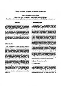
position-pair-coupling-error (PPCE) is found. Performance of the GNN ranking scheme can therefore be quantitatively measured by the PPCE rate. 4.2 Experimental Results We found that the computational demand of the attack graph generation method in [11] is high. The generation of a single real world attack graph took several hours, and hence, we were not able to produce more than 14 graphs within a reasonable time frame for the experiments. The 14 attack graphs were generated using the same computer network example as in a previous work [9], with variations created by adding, removing, or varying vulnerabilities or network configurations. Eight of the attack graphs were randomly selected to form the training data set of the GNN. The remaining six attack graphs are used as the testing data set so as to examine the GNN’s generalization ability in different situations. The GNN used for our experiments consists of two hidden layers, and each hidden layer has 5 neurons. The number of external inputs is also set to 5. Such a GNN has been shown to be successful when applied to ranking web pages [4, 13], and it produces a sufficiently small network that allows for a fast processing of the data. However, this GNN was used successfully on a problem involving much larger number of nodes, and hence, it may be possible to use a somewhat smaller network when dealing with attack graphs. This is not attempted in this paper and may be considered as a topic for future work. We varied the number of training epochs from 500 to 20,000 and repeated the experiment 6 times with randomized initial weights of the underlying MLPs. The PPCE rate results are plotted in Fig. 3. It can be observed that when trained for a sufficiently large number of epochs (around 10,000) the PPCE rate reduces asymptotically to an optimal value. Improvement by further training can be observed but is not significant. Hence the number of training epochs is fixed to be 10,000 in the rest of the experiments for an appropriate effort/time tradeoff. However when applied to ranking attack graphs in practice the training epoch can be set to 20,000 or larger for more accurate results. 0.3

Errorbars Linear interpolation of averages

PPCE Rate

0.25 0.2 0.15 0.1 0.05 0 100

1000 Number of training epochs

10000

Fig. 3. Effect of number of training epochs

From the above experimental results, it can be observed that the average PPCE rate can be reduced to around 10% when GNN is trained with sufficient number of training examples and training epochs. That being the case on an average the proposed GNNbased ranking scheme sacrificed around 10% accuracy in terms of relative position preservation. However, once trained, a GNN can produce output at an O(N ) time complexity where N is the size of input. This may be an improvement compared with the O(N log 1² ) computational complexity required by PageRank. Moreover, the generalization ability of GNN allows us to train GNN on only a small number of attack graphs and apply the results to unseen attack graphs. Figure 4 plots the RPDs resulting from ranking graphs from the testing data set with GNN to visualize the effectiveness of relative position preservation. Each subgraph represents the resulting RPD for one of the 6 attack graphs in the testing data set, and hence it is of different scale to other subgraphs. It can be observed that the order of

ranks are preserved to a reasonable degree. Although only a relatively small portion of nodes remains at exactly the same position as the PageRank scheme, most nodes remain centered around the diagonal and as a result important nodes remain important and unimportant nodes remain unimportant. The GNN-based ranking scheme therefore allows a system administrator to focus on most of the important nodes in an attack graph. 45

45

35

40

40

30

35

35

30

30

25

25

20

20

20

15

15

15

10

10

5

5

0

0

0

5

10

15

20

25

30

35

40

45

25

10 5

0

5

10

15

20

25

30

35

40

45

0

0

40

20

40

35

18

35

16

30

12

25

20

10

20

15

8

15

6

0

5

10

15

20

25

30

35

0

40

20

25

30

35

5

2 0

15

10

4

5

10

30

14

25

10

5

0

5

10

15

20

0

0

5

10

15

20

25

30

35

40

Fig. 4. Relative Position Diagram when trained on real-world attack graphs

Finally, we experimented with reducing the number of training samples. The number of training attack graphs in the training data set is reduced from 8 to 2. The effect on reducing the number of attack graphs used in the training data set is plotted in Figure 5. It can be observed that the number of attack graphs in the training data set has a significant impact on the accuracy in terms of relative positions on the training results. Sufficient attack graphs must be provided in the training data set to simulate the ranking scheme effectively. 0.3

Linear interpolation Points of meassurement

PPCE Rate

0.25 0.2 0.15 0.1 0.05 0 2

3 4 5 6 7 Number of Attack Graphs in training set

8

Fig. 5. Effect of number of attack graphs used in the training data set

4.3 Training with Pseudo Attack Graphs Generating a large number of attack graphs for the training data set is difficult due to significant manual labor and computational effort that it requires [11]. In the following, we provided an alternative scheme for automated training set generation, and train GNN

with automatically generated pseudo attack graphs that have similar shapes and node connection patterns to those of manually generated realistic attack graphs. That attack graphs are non-cyclic, tree shaped graphs resulting from a procedure as follows: at the initial system state, the intruder looks for an entry point and reaches the first layer of nodes in the attack graph by exploiting one of the vulnerabilities applicable to the initial state. With the escalated privilege by the initial exploit, the intruder obtains more intrusion options for the next intrusion step. This procedure repeats and keeps expanding the attack graph until the intruder can reach the intrusion goal. Leaf nodes in the attack graph are thus produced, and the attack graph begins to contract until all attack paths reach the intrusion goal. We generate pseudo attack graphs by simulating this procedure. A pseudo attack graph begins with the root node representing the initial state. It then expands with increasing number of nodes at each layer to simulate the expanding process of realistic attack graphs. This repeats until presumably the intruder begins to reach his goal. Then the pseudo attack graph contracts till all paths are terminated at a leaf node. We repeat the experiments on the same 6 testing attack graphs but using pseudo attack graphs generated by the above procedure as the training data set. In total, 40 pseudo attack graphs are included in the training data set, and GNN is trained for 10,000 epochs for the asymptotic optimal result. The resulting Relative Position Diagrams are as shown in Figure 6. It can be observed that orders of ranks are preserved also to a reasonable degree, but these results are not as accurate as those obtained when using real attack graphs in the training data set. Table 1 lists maximum and minimum PPCE rate by repeating each experiment 3 times. The average PPCE is between 12% to 16%, indicating that on an average the proposed GNN-based ranking scheme sacrificed around 12% to 16% accuracy in terms of relative position preservation. Therefore, using pseudo attack graphs decreases the accuracy by around 2% to 4% compared with using real attack graphs for training, but on the other hand it significantly reduces the effort required to generate real attack graphs. 45

45

35

40

40

30

35

35

30

30

25

25

20

20

20

15

15

15

10

10

5

5

0

0

5

10

15

20

25

30

35

40

45

0

25

10 5

0

5

10

15

20

25

30

35

40

45

0

0

40

20

40

35

18

35

16

30 25

12

25

20

10

20

15

8

15

6 2

0

0

0

5

10

15

20

25

30

35

40

15

20

25

30

35

10

4

5

10

30

14

10

5

5 0

5

10

15

20

0

0

5

10

15

20

25

30

35

40

Fig. 6. Relative Position Diagram when training on pseudo attack graphs

5 Conclusions This paper produced evidence that the GNN model is suitable for the task of ranking attack graphs. GNN learns a ranking function by training on examples and generalizes the function to unseen data. It thus provides an alternative and time-efficient ranking scheme for attack graphs. The training stage for GNN, which is required only once, may

AG-1 AG-2 AG-3 AG-4 AG-5 AG-6 Avg Min PPCE 0.16 0.11 0.14 0.12 0.12 0.11 0.12 Max PPCE 0.21 0.15 0.19 0.17 0.15 0.15 0.16 Table 1. Position Pair Coupling Error

take a relatively long period of time compared with e.g. PageRank scheme. However, once trained the GNN may compute ranks faster than that required by the PageRank scheme. Another advantage of using a machine learning approach is their insensitivity to noise in a dataset. This is a known property of GNN which is based on the MLP architecture. Existing numeric approaches such as PageRank or rule based approaches are known to be sensitive to noise in the data. The GNN provides much more flexible means for ranking attack graphs. A GNN can encode labels that may be attached to nodes or links, and hence, is able to consider additional features such as the cost of an attack or time required for an exploit. This is not possible with the PageRank scheme which is strictly limited to considerations of the topology features of a graph. We plan to investigate how the ability to encode additional information can help to rank attack graphs in the future. Despite the proven ability of the GNN to optimally encode any useful graph structure [12], the result in this paper showed that the performance of the GNN has a potential for improvements. We suspect that this may be due to the choice of training parameters, or the chosen configuration of the GNN. A more careful analysis into this issue is left as a future task.

References 1. Bhadeshia, University Of Cambridge. Neural Networks in Materials Science. 2. E. Mizutani, S. E. Dreyfus. On complexity analysis of supervised MLP-learning for algorithmic comparisons. In International Joint Conference on Neural Networks (IJCNN), volume 1, 2001. 3. F. Scarselli, A. C. Tsoi, M. Gori, and M. Hagenbuchner. A new neural network model for graph processing. Technical Report DII 1/05, University of Siena, Aug 2005. 4. F. Scarselli, S. L. Yong, M. Hagenbuchner, A. C. Tsoi. Adaptive Page Ranking with Neural Networks. In WWW (Special interest tracks and posters), pages 936–937, 2005. 5. P. Frasconi, M. Gori, and A. Sperduti. A general framework for adaptive processing of data structures. 9(5):768–786, September 1998. 6. S. Haykin. Neural Networks, A Comprehensive Foundation. Macmillan College Publishing Company, Inc., 866 Third Avenue, New York, New York 10022, 1994. 7. K. Hornik, M. Stinchcombe, and H. White. Multilayer feedforward networks are universal approximators. Neural Networks, 2(5):359–366, 1989. 8. R.A. Kemmerer, M. Catherine, and Millen J.K. Three system for cryptographic protocol analysis. Cryptology, 7(2):79–130, 1994. 9. L. Lu, J. Horton, R. Safavi-Naini, W Susilo. An Adversary Aware and Intrusion Detection Aware Attack Model Ranking Scheme. In Proceeding of 5th International Conference on Applied Cryptography and Network Security (ACNS 07), Zhuhai, China, Jun 2007. Springer. 10. M. Bianchini, M. Gori, and F. Scarselli. Inside PageRank. ACM Transactions on Internet Technology, 5(1):92–118, Feb 2001. 11. O. Sheyner, J. Haines, S. Jha, R. Lippmann, and J. Wing. Automated generation and analysis of attack graphs. In Proceedings of the IEEE Symposium on Security and Privacy, Oakland, CA, May 2002. 12. F. Scarselli, M. Gori, A.C. Tsoi, Hagenbuchner M., and G. Monfardini. Computational capabilities of graph neural networks. IEEE Transactions on Neural Networks, volume 20(number 1):81–102, January 2009. 13. F. Scarselli, S.L. Yong, M. Gori, M. Hagenbuchner, A.C. Tsoi, and M. Maggini. Graph neural networks for ranking web pages. In Web Intelligence Conference, pages 666–672, 2005. 14. A.C. Tsoi, M. Hagenbuchner, and F. Scarselli. Computing customized page ranks. ACM Transactions on Internet Technology, volume 6(number 4):381 – 414, November 2006. 15. V. Mehta, C. Bartzis, H. Zhu, E. Clarke and J. Wing. Ranking Attack Graphs. In Proceeding of the 9th International Symposium On Recent Advances In Intrusion Detection, Hamburg, Germany, September 2006. Springer.