Ray Tracing Dynamic Scenes using Selective Restructuring. Sung-Eui Yoon1. Sean Curtis2. Dinesh Manocha2. 1Lawrence Livermore National Laboratory.
Eurographics Symposium on Rendering (2007) Jan Kautz and Sumanta Pattanaik (Editors)
Ray Tracing Dynamic Scenes using Selective Restructuring Sung-Eui Yoon1 1 Lawrence
Sean Curtis2
Dinesh Manocha2
2 University of North Carolina at Chapel Hill Livermore National Laboratory Project URL: http://gamma.cs.unc.edu/SR
Abstract We present a novel algorithm to selectively restructure bounding volume hierarchies (BVHs) for ray tracing dynamic scenes. We derive two new metrics to evaluate the culling efficiency and restructuring benefit of any BVH. Based on these metrics, we perform selective restructuring operations that efficiently reconstruct small portions of a BVH instead of the entire BVH. Our approach is general and applicable to complex and dynamic scenes, including topological changes. We use the selective restructuring algorithm to improve the performance of ray tracing dynamic scenes that consist of hundreds of thousands of triangles. In our benchmarks, we observe up to an order of magnitude improvement over prior BVH-based ray tracing algorithms.
1. Introduction Ray tracing has been widely researched due to its ability to generate realistic images. However, the performance of current ray tracing algorithms is considerably slower than GPUbased rasterization algorithms, especially on dynamic scenes. In this paper we address the problem of efficient computation of bounding volume hierarchies (BVHs) of dynamic scenes for faster ray tracing. BVHs have been widely used as an acceleration data structure for ray tracing [RW80, KK86], visibility, and proximity computations [LM03, TKH∗ 05]. A BVH is a hierarchy of bounding volumes (BVs) such that the BV at each internal node encloses the geometric primitives and the BVs associated with its descendants. BVHs are constructed in such a manner as to maximize culling efficiency. Ideally, we would like to compute BVHs with high culling efficiency so that they result in fewer false positives in terms of intersection tests. Recently, BVHs have been used for interactive ray tracing of dynamic models [WBS07, LYTM06, CSE06, LAM03b]. Many dynamic scenes consist of one or more moving objects that may undergo non-rigid or deformable motion. These include changes in the topology due to explosions, cutting, tearing or fracture. Such scenarios arise frequently in gaming, simulation, computer animation, and other applications. In these dynamic environments, a BVH computed for the previous frame may not provide high culling efficiency for the current frame and needs to be updated or recomputed. At a broad level, there are two kinds of approaches to recompute the BVH [TKH∗ 05, OCSG07, LYTM06]. The first set of algorithms restructure the BVHs by either reconstructing the entire BVH or a subset of the BVH. This is achieved c The Eurographics Association 2007.
by recursively partitioning an input set of primitives of a node into multiple disjoint sets of primitives of child nodes such that the BVs associated with child nodes have higher culling efficiency. Although this method can compute BVHs with high culling efficiency, the complexity of these hierarchy construction algorithms on a node with k primitives is typically O(k log k). Since this method has super-linear time complexity, it can be slow for large dynamic models consisting of several hundreds of thousands or more triangles. The second set of methods refit the extents of the BV of each node such that the BV tightly encloses its associated primitives. This involves no re-partitioning of primitives and the BVH can be updated in linear time by traversing the BVH in a bottom-up manner. However, the culling efficiency of the refit BVH may degrade after a few frames (e.g. on scenes with explosions); therefore, the refit BVH may result in too many false positives in terms of intersection tests. Main Results: We present a novel algorithm to selectively restructure a BVH for ray tracing dynamic scenes. Our approach detects small subsets of the BVH that have low culling efficiency and restructures only those subsets. The rest of the BVH is updated using the linear time refitting algorithm. In order to robustly identify the subsets of the BVH, we introduce two metrics: • Culling efficiency metric: This metric probabilistically estimates the culling efficiency of a BVH or a sub-BVH in terms of the number of ray intersection tests performed during the BVH traversal. This metric is based on surface-area heuristic (SAH) [GS87]. • Restructuring benefit metric: This metric is a probabilistic model that estimates the benefit of restructuring a subset of the BVH in terms of improved culling efficiency.
S. Yoon & S. Curtis & D. Manocha / Ray Tracing Dynamic Scenes using Selective Restructuring
Figure 1: Exploding dragon benchmark: Three images are shown from a dynamic simulation of a bunny breaking a dragon. This scene consists of 252K triangles and undergoes drastic topological changes. We use our algorithm to selectively restructure an axis-aligned bounding box (AABB) tree during each frame. Our ray tracing algorithm based on selective restructuring is able to achieve 65%–1000% performance improvement over prior ray tracing algorithms that are based on AABB-trees. We present simple and efficient algorithms to compute these metrics. Our selective restructuring algorithm traverses the BVH in a top-down manner and performs incremental restructuring operations based on these metrics. We demonstrate the benefits of selective restructuring for ray tracing dynamic scenes. We use an optimization approach that reduces the total frame time, including BVH restructuring operations and ray intersection tests during BVH traversal. We have tested the performance of our algorithm on a wide range of benchmarks, consisting of tens or hundreds of thousands of triangles and varying levels of dynamic behavior. In practice, selective restructuring takes a small fraction of the overall frame time and can significantly improve the culling efficiency of the BVH. We also compare the performance with prior BVH-based ray tracing algorithms and observe up to one order of magnitude performance improvement on our benchmarks. As compared to prior BVH-based ray tracing algorithms, our approach offers the following benefits: 1. Generality: Our algorithm works with various types of BVHs and arbitrary deformation including topological changes. Furthermore, our algorithm can be combined with other hierarchy construction methods. 2. Formal models: Our approach is based on two probabilistic metrics that quantify the culling efficiency and restructuring benefit of BVHs. As a result, our dynamic BVH restructuring algorithm works well on different kinds of dynamic models. 3. Complex models: The overhead of performing our selective restructuring operation is relatively small. Also, our BVH restructuring algorithm scales well to large dynamic models. 4. Faster ray tracing: Our ray tracing algorithm can offer significant performance improvement over prior dynamic BVH-based approaches.
Figure 2: BART benchmark: This figure shows three images from the well known BART benchmark with 16K triangles ([LAAM01]). We use our selective restructuring algorithm to recompute the AABB-tree for ray tracing this model. We compare our algorithm with four prior approaches and observe 11 − 2700% performance improvement on this benchmark. Organization: The rest of the paper is organized as follows: Sec. 2 gives a brief summary of prior work on hierarchy update methods and ray tracing dynamic scenes. We give an overview of our approach and describe the basic restructuring operation in Sec. 3. We present our two metrics in Sec. 4 and use them to formulate the selective BVH restructuring algorithm for ray tracing in Sec. 5. We highlight the performance on different benchmarks in Sec. 6. Finally, we analyze the performance of our algorithm in Sec. 7.
2. Related work In this section we give a brief overview of prior work on BVHs as well as the refitting and restructuring algorithms for ray tracing dynamic scenes. 2.1. Bounding Volume Hierarchies There are different types of BVs. Some of the commonly used BV types include simple shapes such as spheres [Hub93, BO04] and axis-aligned bounding boxes (AABBs) [vdB97], or tight fitting BVs such as oriented bounding boxes (OBBs) [GLM96], spherical shells [KPLM98] and discretely oriented polytopes (k-DOPs) [KHM∗ 98], etc. Many hybrid combinations that use more than one BV in a hierarchy or combine them with spatial partitioning methods have also been proposed [LGLM99, SM04] Many top-down and bottom-up techniques have been proposed to construct these BVHs [LM03, TKH∗ 05]. 2.2. Hierarchies for Dynamic Scenes The problem of building good hierarchies for dynamic datasets has been addressed in computer graphics, computational geometry, and database literature. An excellent recent survey is given in [Sam06]. These include specialized hierarchies like parametric R-tree and TPR-tree for time parametric rectangles or fieldtrees for objects undergoing relatively little motion. Most of the algorithms in computer graphics or interactive applications use simple BVs such as spheres or AABBs and recompute the BVH. The simplest algorithms update or refit each BV and take linear time in the number of nodes in the tree [LAM06]. Many specialized refitting algorithms have c The Eurographics Association 2007.
S. Yoon & S. Curtis & D. Manocha / Ray Tracing Dynamic Scenes using Selective Restructuring
also been presented for bounded deformations [JP04], morphing objects [LAM03a], and kinetic data structures [ZW06]. The restructuring algorithms reconstruct the entire BVH or a subset of the BVH at each frame [TKH∗ 05]. However, prior algorithms can be slow in practice on large dynamic models with hundreds of thousands of primitives. Many techniques have been proposed to improve the performance of the entire tree construction algorithms [WK06, HMS06, PGSS06], detect the quality degradation of BVHs and mesh clusters [Sam06, LAM06, CH04], or perform dynamic restructuring for fracturing objects [OCSG07]. 2.3. Ray Tracing and Intersection Computations Spatial partitioning and BVHs have been widely used to accelerate ray tracing and intersection computations. Interactive ray tracing of dynamic scenes has received considerable attention in the last few years [LAAM01, WBS03]. These include algorithms that combine BVHs with spatial partitioning hierarchies [GFW∗ 06, HHS06, WMS06, WK06] or use a combination of refitting or reconstruction algorithms [WBS07, LYTM06]. We compare our method with prior BVH-based ray tracing methods in Section 6.
3. Overview In this section we give an overview of our approach and introduce the notation used in the paper. Our algorithm takes input dynamic scenes as polygon soup models and does not assume any particular deformations on the input scenes. Bounding Volume Hierarchies: Each node in a BVH has a bounding volume (BV), which can be used for ray intersection queries. The leaf nodes of a BVH contain primitives (e.g., triangles) contained in the BV of the node. Ideally, we would like to compute a tight fitting BV for each internal node that encloses all the primitives within its descendant nodes. Our algorithm does not make any assumptions about the type of BV. However, we assume that the BVH represents a layered hierarchy [GNRZ02], where a BV at an internal node encloses the BVs of its child nodes. For simplicity, we assume a binary BVH. However, our algorithm can be easily extended to n-ary BVHs. Also, our approach does not make any assumptions about the specific construction algorithm used to partition the primitives belonging to the entire BVH or a subset of the BVH. Notation: For the rest of the paper, we use the symbol n to denote a node and BV(n) to denote the BV associated with a node n. The term sub-BVH(n) denotes the subtree that is rooted at n and includes all the descendants of n. We use the symbol nˆ to denote a node that is obtained after applying our restructuring operation to sub-BVH(n). Let Le f t(n), Right(n), and Parent(n) denote the left child, right child, and parent node of n, respectively, and nRoot be the root node of the BVH. The symbol |n|tri denotes the number of triangles contained in sub-BVH(n). 3.1. BVH Restructuring The simplest algorithms for dynamic BVHs are based on BV refitting. These are simple to implement and quite fast due to their linear time complexity. Moreover, refitting alc The Eurographics Association 2007.
Figure 3: Performance of Different Methods: The left graph shows the relative total rendering time of ray tracing breaking bunny and dragon models consisting of 252K triangles during 80 frames (Fig. 1). Our selective restructuring algorithm shows more than one order of magnitude improvement over "BV-refitting only" method and 6 times improvement over complete BVH restructuring method optimized with surface-area heuristic (SAH). This performance improvement is achieved by selectively restructuring sub-BVHs only when we can improve the overall performance of ray tracing. The right graphs show the number of intersection tests at each frame; the inset in the right graph shows zoomed view of the graph. Our method shows more than 20 times improvement over "BV-refitting only" method. gorithms based on AABB trees can be an order of magnitude faster than complete reconstruction algorithms for AABB trees [TKH∗ 05, vdB97]. In practice, complete reconstruction algorithms can take many seconds on models with 100K − 500K triangles. At the same time, BVHs updated by using BV refitting methods can have poor culling efficiency. One such example is shown in Fig. 3, which shows the number of intersection tests per frame performed during ray tracing a dynamic scene with breaking objects as shown in Fig. 1. The number of intersection tests on the dynamic BVH computed using the refitting algorithm is two orders of magnitude higher, as compared to that on the dynamic BVH computed using complete reconstruction. In order to overcome these performance issues, we present a selective BVH restructuring algorithm that only restructures small subsets of the BVH that have low culling efficiency. This is demonstrated in Fig. 3, where the culling efficiency of the dynamic BVH computed by our algorithm is comparable to that of the complete reconstruction algorithm. Moreover, the time spent in restructuring operations by our selective BVH restructuring algorithm is a fraction of that spent by the complete reconstruction algorithm. In order to perform restructuring operations, our algorithm uses two metrics, as mentioned in Sec. 1. These metrics evaluate the culling efficiency of a given sub-BVH as well as the restructuring benefit, which measures the improvement in culling efficiency due to selective restructuring. Next, we introduce the basic restructuring operation used by our algorithm.
S. Yoon & S. Curtis & D. Manocha / Ray Tracing Dynamic Scenes using Selective Restructuring
4. BVH Metrics In this section we introduce two novel metrics that are used to perform selective restructuring. First, we present our culling efficiency metric that measures the expected number of intersection tests performed during ray tracing. Next, we present the restructuring benefit metric, which estimates the improvement in culling efficiency due to the restructuring operation described in Section 3.2. These metrics are applicable to all BVHs. Figure 4: Basic restructuring operation: Our algorithm selects a node pair (n1 , n2 ), whose BVs overlap considerably (show on the left). Our restructuring operations takes the union of primitives contained in sub-BVH(n1 ) and subBVH(n2 ), re-partitions the primitives into two new nodes, nˆ1 and nˆ2 , and recursively process the sub-BVHs of the new nodes. The complexity of this operation is O(klogk), where k = |n1 |tri + |n2 |tri . This is in contrast with other restructuring algorithms where k = |nA |tri , where nA is the lowest common ancestor of n1 and n2 . 3.2. Selective Restructuring Operation Our algorithm performs selective restructuring operations in an incremental manner. Each operation evaluates a pair of nodes in the BVH, say (n1 , n2 ), shown in Fig. 4. These can be any two nodes of the BVH, as long as one of them is not an ancestor of another. Let nA be the lowest common ancestor of both of these nodes. Our algorithm computes the extent of overlap between BV(n1 ) and BV(n2 ). If there is a high degree of overlap between these BVs, this node pair is a good candidate for restructuring operation. This is based on the fact that a high degree of overlap between the BVs can lead to poor culling efficiency. In order to perform the restructuring operation, we use our metrics to estimate the culling efficiency and restructuring benefit of sub-BVH(n1 ) and sub-BVH(n2 ), before and after the restructuring operation. Based on these metrics, our algorithm determines whether this pair is a good candidate for performing the restructuring operation. If so, we take the union of all the primitives in sub-BVH(n1 ) and sub-BVH(n2 ) and re-partition the primitives in that union into new nodes nˆ1 and nˆ2 , as shown in Fig. 4. Therefore, the BVs of new nodes would have considerably less overlap. The major advantage of our selective restructuring operation is that it is localized and only a small number of the primitives are re-partitioned or re-grouped during this operation. For example, if we restructure a single node and its sub-tree to minimize the overlap between BV(n1 ) and BV(n2 ), that node would be the common ancestor of n1 and n2 (i.e. nA ). Since the number of primitives associated with sub-BVH(n1 ) and sub-BVH (n2 ) can be much lower as compared to that with sub-BVH (nA ), the cost of our selective restructuring operation is lower than that of reconstructing only a single node of the BVH.
4.1. Cost Model for Intersection Queries An intersection query is the basic geometric operations performed during BVH traversal. In ray tracing there are two types of intersection tests: ray-BV and ray-primitive tests. The traversal algorithm starts from the root node and performs these intersection tests in a recursive manner. If there is an intersection with a node, it recursively checks for intersection with its children. Otherwise, it terminates. At the leaf nodes, the algorithm performs intersection tests with the primitives (e.g., triangles). We define the probabilistic cost model of intersection query, CM-IQ, of a node n. CM-IQ measures the expected number of intersection tests performed during an intersection query that starts at sub-BVH(n), given that there is an intersection with BV (n). We relate this model with the culling efficiency of sub-BVH(n). A higher value of CM-IQ implies low culling efficiency of the sub-BVH. 4.1.1. CM-IQ Derivation Let C(n) denote the value of CM-IQ associated with subBVH(n). Also, let P(n) denote the probability that a node n will be accessed during an intersection query. Then, by the definition of intersection query described above, we can define C(n) in a recursive manner as: |n|tri ∗Clea f , if n is a leaf node 1 + P(Le f t(n)) ∗C(Le f t(n))+ C(n) = P(Right(n)) ∗C(Right(n)), otherwise, (1) where Clea f is the relative cost of performing an intersection test with a primitive (e.g. a triangle) compared to the cost of an intersection test with a BV. We include Clea f to consider the costs of intersection tests with primitives and BVs in one metric. Later, we will describe a simple method to automatically compute Clea f . In order to compute CM-IQ for each node, we need to compute the probability, P(n), that a node n is accessed given that its parent node Parent(n) is accessed during the intersection query. This probability formulation is well known in ray tracing literature as the surface-area heuristic (SAH) [GS87, MB90, Hav00, WH06] and is defined as: P(n) =
Area(n) , Area(Parent(n))
(2)
where Area(n) is the surface-area of the BV of the node n. For more general intersection queries between the BVs, we could also use the volume-based formulation proposed in [YM06]. c The Eurographics Association 2007.
S. Yoon & S. Curtis & D. Manocha / Ray Tracing Dynamic Scenes using Selective Restructuring
Figure 5: Accuracy of CM-IQ metric: This graph shows values of our CM-IQ metric based on surface-area heuristic (SAH) and the number of ray intersection tests observed during ray tracing of N-body simulation shown in Fig. 8. Although the intersection tests are measured from a certain view point, there is strong correlation (0.85) between them. This indicates a high degree of accuracy of our CM-IQ metric. Please note that our CM-IQ measures the expected number of intersection tests given that a ray intersects with BV(n Root ), the BV of the root node of a BVH. To estimate the total number of intersection tests performed during ray tracing at an entire frame, we need to multiply the CM-IQ value by the number of such rays intersecting BV(nRoot ). Since we do not know the number of such rays at a frame, we estimate it with that of the previous frame. For the sake of simplicity, we choose to omit this factor in the derivations for the rest of the paper. Cost Value Decomposition Property: Suppose that the BV of a node n can be decomposed into two virtual disjoint child nodes a and b, i.e., BV (a) ∩ BV (b) = ∅. Then, the following equation holds, based on conditional probability: C(n) = C(a ∪ b) =
Area(a) Area(b) C(a) + C(b). Area(n) Area(n)
(3)
We use this property to explain a derivation of our restructuring benefit metric later. Evaluating CM-IQ: The simplest method to evaluate CM-IQ is to recursively apply Eq. (1) to sub-BVH(n). This method assumes that all the nodes of the sub-BVH rooted at node n will be accessed during ray-BV intersection queries. However, many of the descendant nodes may not be accessed due to various geometric factors (e.g., visibility) during a frame. In order to efficiently take this property into account, we use frame-toframe coherence to estimate which nodes would be accessed in the current frame based on the nodes that were accessed during the previous frame. Eventually, we evaluate our metric only on those nodes. We associate a time-stamp variable with each node of the BVH and update the variable for the nodes that are accessed. We have empirically verified the accuracy of CM-IQ metric by computing a linear correlation between values of CM-IQ computed by our algorithm and the number of intersection tests observed during ray tracing. We observe a high linear correlation ranging from 0.7 to 0.9 in our benchmarks. This is illustrated in a correlation graph shown in Fig. 5. 4.2. Restructuring Benefit Model We now present our restructuring benefit model for ray intersection query, which predicts the expected improvement in c The Eurographics Association 2007.
Figure 6: Classification of Overlapping Regions: This figure illustrates the overlapping regions between the BVs of two nodes, n and n. ˆ Note that nc , n− , and n+ are regions that belong to both BV (n) and BV (n), ˆ only BV (n), and only BV (n), ˆ respectively. culling efficiency during restructuring operations. We define restructuring benefit model of intersection queries, RM-IQ, to estimate the benefit of performing the restructuring operation on sub-BVH (n1 ) and sub-BVH (n2 ), given a node pair, (n1 , n2 ). The restructuring operation would compute a new node pair (nˆ1 , nˆ2 ). The benefit is computed in terms of improved culling efficiency, i.e., reduction in the number of intersection tests. Let R(n1 , nˆ1 , n2 ) represent the expected reduction in the number of intersection tests due to the new node, nˆ1 , and its sub-BVH. In the same manner, our restructuring algorithm also computes R(n2 , nˆ2 , n1 ). 4.2.1. RM-IQ Formulation Let ∆C(n1 , nˆ1 , n2 ) represent the difference, C(n1 ) − C(nˆ1 ), in the expected number of intersection tests before and after restructuring. This is based on the condition that the rebuilt node nˆ1 is accessed during the traversal. Then, we represent R(n1 , nˆ1 , n2 ) as: R(n1 , nˆ1 , n2 ) = ∆C(n1 , nˆ1 , n2 )P(nˆ1 ).
(4)
Our goal is to estimate this term without explicitly computing nˆ1 and its sub-BVH (nˆ1 ). We cannot exactly compute P(nˆ1 ), as it requires actually performing the restructuring operation and computing nˆ1 . Instead, we simply use the probability, P(n1 ), as an approximation for P(nˆ1 ). 4.2.2. Derivation of ∆C(n1 , nˆ1 , n2 ) In order to estimate ∆C(n1 , nˆ1 , n2 ), we need to estimate C(nˆ1 ), which in turns depends on BV(nˆ1 ). To do that, let us decom+ pose BV(n1 ) ∪ BV(nˆ1 ) into three regions: nc1 , n− 1 , and n1 that belong to both BV (n1 ) and BV (nˆ1 ), only to BV (n1 ), and only to BV (nˆ1 ), respectively (see Fig. 6). The superscripts c, −, and + indicate the areas that are common, deleted, and added, respectively, after restructuring the node n to n. ˆ Intuitively speaking, the culling efficiency after restructuring will be improved as the region of n− 1 increases and the regions of n+ decreases. 1 Given the decomposition of BV(n1 ) ∪ BV(nˆ1 ), we derive the following equation, obtained by expanding our cost model based on cost value decomposition property introduced in Sec-
S. Yoon & S. Curtis & D. Manocha / Ray Tracing Dynamic Scenes using Selective Restructuring
Based on these assumptions, ∆C(n1 , nˆ1 , n2 ) can be approximated as:
tion 4.1.1: c + C(n1 ) −C(nˆ1 ) =C(nc1 ∪ n− 1 ) −C(n1 ∪ n1 )
=
Area(n− Area(nc1 ) c 1 ) C(n− ) 1 − C(n1 ) + c Area(n1 + n1 ) Area(nc1 + n− 1 )
−
Area(n+ Area(nc1 ) c 1) C(n+ 1 ). + C(n1 ) − c Area(n1 + n1 ) Area(nc1 + n+ ) 1 (5)
It follows that ∆C(n1 , nˆ1 , n2 ) increases as the region corre+ sponding to n− 1 increases and n1 decreases. However, the − region corresponding to n1 mainly depends on the overlap region between BV(n1 ) and BV(n2 ). Moreover, we do not know these regions exactly without explicitly computing nˆ1 and BV(nˆ1 ). We present a simple and efficient approximation method to compute ∆C(n1 , nˆ1 , n2 ) without actually computing nˆ1 . The main observation behind our approximation is the property that the overlap region between two BVs is likely to be reduced after a restructuring operation. 4.3. Approximation of ∆C(n1 , nˆ1 , n2 ) In order to approximate the difference, ∆C(n1 , nˆ1 , n2 ), we make the following three assumptions: • Complete Removal of BV Overlap: The improvement in culling efficiency after restructuring will increase as re+ gion n− 1 increases and region n1 decreases according to Eq. (5). If there is considerable overlap between BV(n1 ) and BV(n2 ), that overlap can be reduced by restructuring the two nodes and all the primitives contained in sub-BVH (n1 ) and sub-BVH(n2 ). Therefore, it is likely that the region n− 1 would increase when the overlap between BV(n 1 ) and BV(n2 ) is higher. We assume that any reasonable reconstruction method will reduce most of the overlapping region by restructuring primitives associated with two overlapping nodes. Particularly, we assume that the entire overlapping region will be eliminated. For example, if we use AABB as BVs, half of the surface areas of faces of the overlapping region, except for faces parallel to the dividing plane, will be reduced from Area(n1 ). Let Area(nr1 ) denote the extent of such a reduced area. • Ignoring n+ 1 : We assume that the reconstruction algorithm will construct new BVs such that they minimize this region. Therefore, we do not take the region of n+ 1 into account during our approximation. The BV example shown in Fig. + 4 also does not introduce n+ 1 nor n2 after restructuring. • Linear Approximation: In order to approximate the differences in the culling efficiency shown in Eq. (5), we need to compute C(nc1 ). We assume that the geometric primitives are uniformly distributed in BV (n1 ). Then, we linearly approximate C(nc1 ) based on the ratio of surface areas of region of nc1 to that of BV (n1 ). Therefore, C(nc1 ) can be apArea(nc ) proximated as Area(n1 ) C(n1 ). 1
C(n1 ) −C(nˆ1 ) ≈ C(n1 ) −C(nc1 ) ≈ C(n1 ) − ≈ C(n1 )
Area(nr1 ) . Area(n1 )
Area(nc1 ) C(n1 ) Area(n1 )
(6)
To verify the accuracy of these approximations, we measured how much the observed cost values deviate from the expected cost values in terms of surface areas of BVs. 80% of observed values are within 25% of the expected value. Moreover, the standard deviations of ratios of those 80% observed values to the expected values are within 0.08 across our benchmarks. Therefore, the expected values are very close to the observed values on average. However, in the other 20% observed values, our simple approximation can result in significant errors depending on configurations. In the worst cases, the observed values were two times bigger than the expected values. Final RM-IQ: After substituting all the equations into our RM-IQ formulation shown in Eq. (4), we obtain the following approximation of our restructuring metric, RM-IQ: R(n1 , nˆ1 , n2 ) = C(n1 )
Area(nr1 ) P(n1 ). Area(n1 )
(7)
Our restructuring algorithm reconstructs two nodes, n1 and n2 , and their sub-BVHs only if R(n1 , nˆ1 , n2 ) + R(n2 , nˆ2 , n1 ) is larger than the restructuring cost, f rebuild (n1 , n2 ), of sub-BVH (n1 ) and sub-BVH (n2 ). The restructuring cost, frebuild (n1 , n2 ), can be computed based on the number of triangles associated with those two sub-BVHs. Typically, the time complexity of a reconstruction method is O(k log k). Therefore, frebuild (n1 , n2 ) = Crebuild ∗ (k log k), where k = (|n1 |tri + |n2 |tri ). Crebuild is a machine-dependent constant used in estimating the cost of the reconstruction algorithm.
5. Ray Tracing with Selective Restructuring In this section, we present our algorithm to efficiently restructure BVHs for ray tracing dynamic scenes. Also, we explain how this selective restructuring algorithm is combined to perform ray tracing. 5.1. Overall Selective Restructuring Algorithm The selective restructuring algorithm is performed at the beginning of each frame. We first perform BV refitting by updating the BVs in a bottom-up manner. However, these refit BVs may have the low culling efficiency. To detect such BVs, we evaluate the culling efficiency metric for each node of the BVH. Next, we perform selective restructuring operations. Our algorithm traverses the BVH and detects sub-BVHs whose culling efficiency can be improved by restructuring them. The main goal of our restructuring algorithm is to minimize the frame time of ray tracing, which is a combination of restructuring time and traversal time of a BVH. In order to achieve this goal, our algorithm computes a set of node pairs, which are candidates for our basic restructuring operations. Each pair, (n1 , n2 ), is associated with two values: 1) the restructuring cost of sub-BVH(n1 ) and sub-BVH(n2 ); and c The Eurographics Association 2007.
S. Yoon & S. Curtis & D. Manocha / Ray Tracing Dynamic Scenes using Selective Restructuring
2) the RM-IQ value shown in Eq. (7). Our overall algorithm proceeds in two phases: hierarchical refinement phase and restructuring phase, as shown in Alg. 1. Next, we describe each of them in more detail. 5.2. Hierarchical Refinement Phase Our algorithm performs the basic restructuring operation defined in Section 3.2. The algorithm starts with selecting two nodes, whose BVs have a high degree of overlap. However, if there are m different BV nodes in a BVH, a naive approach would need to check O(m2 ) node pairs to detect all the overlaps between the BVs. Instead, we traverse an input BVH in a top-down manner and perform hierarchical culling to reduce the number of pairs to be checked for overlap tests. The main motivation of hierarchical culling arises from the following property: if there is no overlap between the BVs of two nodes, there is no overlap between BVs of their descendant nodes. Refinement: We start with an initial pair with the two children of nroot . We also maintain a queue of pair nodes called pairqueue, which serves as a computation front during the topdown BVH traversal. We initialize the queue with the initial pair. The algorithm proceeds by extracting a pair, say (n 1 , n2 ) from the pair-queue, and checking for overlap between the BVs of the two nodes. Based on the overlap, we evaluate the RM-IQ metric for each node and determine whether that pair is a good candidate to perform our restructuring operation. If there is no overlap between BV(n1 ) and BV(n2 ), it is guaranteed that there is no overlap between the BVs of any node in sub-BVH(n1 ) and the BVs of any node in sub-BVH(n2 ). Therefore, we do not need to consider any such pairs for the restructuring operation. However, there can be overlap between two children nodes of n1 or the two children nodes of n2 . Therefore, we add two new pairs, (Le f t(n1 ), Right(n1 )) and (Le f t(n2 ), Right(n2 )) to the pairqueue. In other words, the pair (n1 , n2 ) is refined into those two pairs. On the other hand, if there is overlap between BVs of two nodes of a pair (n1 , n2 ), this pair is a possible candidate for restructuring operation. Therefore, we also perform a refinement operation to further localize the overlapping area between BV(n1 ) and BV (n2 ). We compare the volumes of both the BVs and select the node with the larger volume, say n 1 . We refine this node with its children, and create two new pairs, (Le f t(n1 ), n2 )) and (Right(n1 ), n2 ). At the same time, we also add another pair (Le f t(n1 ), Right(n1 )) to the pair-queue. Stopping Criteria: There is a cost associated with refining the node pairs and evaluating the RM-IQ metric for the node pairs. Let Cre f ine represent the cost of refining a pair. We refine a pair when it is likely that refinement could result in improving the overall performance. Specifically, we refine a pair if its restructuring benefit is at least bigger than the refinement cost. We define the refinement cost of a pair as a function of the number of nodes in the queue since we have to process all the pairs in the queue before we process the refined pairs. Propagation: When we apply the basic restructuring operation to two nodes of a pair, the overlap between the BVs of the nodes can be reduced. Moreover, restructuring any of the ancestor nodes of those two nodes can reduce the overlap too. However, when we evaluate restructuring benefit only with those ancestor nodes, we cannot foresee such benefit with their c The Eurographics Association 2007.
Algorithm 1 Selective Restructuring Algorithm 1: // Hierarchical Refinement Phase 2: PairQ ← (Left(nRoot ), Right(nRoot )) // Add initial pair to the queue 3: while (! PairQ.empty ()) do 4: Pair ← PairQ.front (); 5: EvaluateRM-IQ (Pair); // Evaluate RM-IQ based on the overlap 6: // Check whether restructuring benefit of a pair is larger than the refining cost 7: if (WorthRefine(Pair)) then 8: PairQ ← Refine (Pair); 9: end if 10: Propagate (Pair); // Propagate RM-IQ value of Pair to pairs, which are refined to Pair 11: end while 12: // Restructuring Phase 13: PairH ← All created pairs // Add the created pairs to the pair heap 14: while (! PairH.empty ()) do 15: Pair ← PairH.front (); 16: // Restructure benefit should be larger than the restructuring cost 17: if (WorthRebuild (Pair)) then 18: (n1 , n2 ) ← Pair 19: RestructureTwoSubBVHs (n1 , n2 ); // Described in Sec. 3.2 20: end if 21: end while
descendant nodes. To address this issue, the restructuring benefit of a pair p1 should be recursively propagated and added to the RM-IQ value associated with a pair, which was refined to p1 . Also, this information is recursively propagated to the very first pair (Le f t(nRoot ), Right(nRoot )). This is because restructuring two child nodes of the root node can reduce all the overlaps between any nodes of the BVH. We perform the propagation right after the refinement operation, as shown in Line 10 of Alg. 1. 5.3. Restructuring Phase In the hierarchical phase, we computed the restructuring benefit of pairs in top-down manner. To maximize the overall performance of ray tracing dynamic scenes, we restructure pairs with higher restructure benefits in a greedy manner. In order to perform this computation, we start the restructuring phase by putting all the pairs created so far into a pair-heap, where the pairs are sorted based on difference between the restructuring benefit and the restructuring cost associated with each pair. As we fetch a pair from the pair-heap, we restructure the two sub-BVHs associated with the pair whenever the restructuring benefit is larger than the restructuring cost. Partitioning Plane: Our goal in performing restructuring operations is to reduce the overlap between BVs of two nodes of a pair. To achieve this goal, we need to compute a partitioning plane that will re-partition triangles associated with two nodes and their sub-BVHs. Suppose that we restructure two nodes n1 and n2 of a pair. Also, suppose that n1 and n2 are descendant nodes of Le f t(nA ) and Right(nA ), respectively,
S. Yoon & S. Curtis & D. Manocha / Ray Tracing Dynamic Scenes using Selective Restructuring
node nˆ can be used for many frames before it will be rebuilt again. Therefore, it is likely that the culling efficiency improvement of nˆ can be observed for many frames. We take this factor into account by introducing the notion of life time of all nodes in the BVH. This expected life time is simply computed as an average life time of all nodes by considering the number of rebuilt nodes and the number of nodes in the BVH from the first frame to the current frame. Since it is likely that we get a higher restructuring benefit on sub-BVHs by restructuring them as the expected life time is getting longer, we simply multiply our final RM-IQ model shown in Eq. (7) by the value of expected life time. Figure 7: Cloth simulation benchmark: Three image sequences are shown among 80 frames from a dynamic sequence of a cloth twisting around a ball. This scene consists of 92K triangles. We compare the performance of different ray tracing algorithms on this scene. The BVH created for the first frame works well for the rest of the frames with simple BV refitting method. Therefore, "BV refitting only" method shows the best performance. However, even in this case, our algorithm shows only 4% worse performance over the refitting algorithm and more than three times improvement over the complete reconstruction algorithm. where nA is the lowest common ancestor of n1 and n2 . We set the partitioning plane to pass the centroid of the overlapping area between BV (Le f t(nA )) and BV (Right(nA )) and the normal of the plane is parallel to a direction that has longest extent of BV (nA ). The main reason that the partitioning plane is computed based on BV (nA ), not based on the local overlap between BV (n1 ) and BV (n2 ), is to minimize or avoid any BV overlap between any ancestor nodes of n1 and n2 . Please note that these ancestor nodes were partitioned to reduce the overlap between BV (Le f t(nA )) and BV (Right(nA )). We observe that our heuristic to compute a partitioning plane works well in our benchmarks. 5.4. Ray Tracing Once we compute a BVH for the dynamic dataset at each frame, we run BVH-based ray tracing algorithm and perform ray intersection queries. BVH-based ray tracing methods have been recently used for interactive ray tracing of dynamic or deformable models. This is due to the fact that it is relatively inexpensive to update a BVH as compared to a kd-tree, which works better for static scenes [LYTM06, WBS07]. We further improve the performance of BVH-based ray tracing based on our selective restructuring algorithm. We use axis-aligned bounding box (AABB) as a BV due to its simplicity and employ a surface-area heuristic [WH06] within our basic selective restructuring operations. The simplest algorithms shoot a ray corresponding to each pixel and perform ray-AABB intersection queries during tree traversal. At each intersection, the algorithm may spin off secondary rays, including shadow rays and reflection rays. The overall performance of ray tracing algorithm is governed by both the restructuring time and tree traversal time. In order to achieve better performance for ray tracing, we further specialize the RM-IQ metric. For example, a rebuilt
6. Implementation and Results In this section, we describe our implementation and the performance improvement for ray tracing dynamic scenes using our algorithm. We highlight its performance on different benchmarks and also compare it with prior restructuring methods as well as ray tracing algorithms. 6.1. Implementation We have implemented our algorithm on a Intel Pentium 4 mobile laptop machine with a 2.1Ghz CPU and 2GB main memory. All the timing data collected in this paper is based on a single-threaded implementation. We use AABB as the BV and implemented an AABB-based ray tracer on dynamic models, as described in Sec. 5.4. Machine-specific constants: The performance of our selected restructuring algorithm depends on machine-dependent constants. These include the cost of reconstructing a sub-BVH (n) (Crebuild (n)), the cost of performing an intersection test with a leaf node vs. the intersection test with a BV, i.e. Clea f = ray-triangle intersection cost ( ray-AABB intersection cost ), and the cost of refining a pair of nodes performed during selective restructuring (Cre f ine ). We also measure Cre f ine and Crebuild as the relative cost to the cost of ray-AABB intersection cost; therefore, all our metrics using these constants are compared in the same unit. We automatically compute these costs by running those routines a few times without any manual intervention during the ray tracing system’s initialization. Then, we use their average values in our algorithm. Once these constants are computed on a machine, these constants are used for all dynamic scenes without any modification. Lazy computations: Many interactive algorithms use a lazy strategy to construct a hierarchy [LAM06]. These algorithms only construct a node of a tree if that node is needed to perform an intersection test during the traversal. Our selective restructuring operation on the pair (n1 , n2 ) also reconstructs the nodes within sub-BVH(n1 ) and sub-BVH(n2 ) in a lazy manner. The new descendants of nˆ1 and nˆ2 are computed in a lazy manner only if they are needed to perform intersection tests during the traversal. Benchmarks: In order to test the performance of our algorithm, we used three types of dynamic scenes. These include: • Deformable models: Models undergoing non-rigid deformation. This type of models is represented by our cloth simulation (with 92K) triangles, shown in Fig. 7. c The Eurographics Association 2007.
S. Yoon & S. Curtis & D. Manocha / Ray Tracing Dynamic Scenes using Selective Restructuring Model Exploding dragon N-body simulation Cloth simulation BART benchmark
Triangles (K) 252 146 92 16
Number of Frames 100 130 80 40
Image Fig. 1 Fig. 8 Fig. 7 Fig. 2
Table 1: Dynamic Benchmark Models: This table shows the complexity of the benchmarks and the number of frames used in our timing computations. • N-body simulations: These consist of multiple moving objects. Each object may undergo a rigid or deformable motion and the objects collide with each other and the ground. We use a simulation of hundreds of moving balls with 146K triangles (Fig. 8). • Breaking objects: In these benchmarks, one or more objects break into smaller pieces (i.e. explosions) and thereby change their topologies. These are some of the most challenging dynamic scenes. We also use the well-known BART benchmark with 16K triangles (Fig. 2) and an "Exploding dragon" benchmark, where a bunny collides with the dragon model and breaks the dragon into numerous pieces (Fig. 1). This model has more than 250K triangles and is a challenging benchmark for many prior algorithms. All of these models have different characteristics and model complexity. As a result, they provide a good suite of benchmarks to test the performance of our algorithm. Detail information about each benchmark is shown in Table 1. 6.2. Performance Comparison We compare the performance of our selective restructuring based ray tracing algorithm with prior ray tracing algorithms that use dynamic BVHs. Specifically, we have compared the performance with four prior approaches: • BV refitting only: In this case, the dynamic BVH is computed by refitting all the BVs in the tree in a lazy manner. This is the cheapest algorithm for recomputing a dynamic BVH and has been used for ray tracing dynamic scenes [WBS07]. Its performance strongly depends on an initially built BVH and can drastically degrade on models with changing topologies. • Complete reconstruction: This algorithm reconstructs a new BVH during each frame using O(k log k) computations. Its performance slows down on large models due to the complexity of the algorithms. • RT-Deform: This is a hybrid refitting/reconstruction algorithm [LYTM06]. By default, this algorithm only refits the BVs during each frame. However, it uses a simple heuristic based on SAH metric to evaluate the culling efficiency of the whole tree. If the culling efficiency is low, this algorithm computes a new BVH using complete reconstruction, and thereby takes a large fraction of the frame time. • LM-reconstruction algorithm: [LAM06] propose a restructuring algorithm that only reconstructs a subset of the BVH. This algorithm was initially designed for collision detection between two objects. However, because the core of the algorithm is focused on detecting BVH degradation and localizing reconstruction, the same approach can also be used to compute a dynamic BVH for ray tracing. We c The Eurographics Association 2007.
LM- RT-DEFORM Refitting Complete BVH algorithm algorithm only Reconstruction Exploding dragon 2.16 1.65 11 8.5 N-body simulation 1.36 1.25 > 80 1.81 Cloth simulation 1.29 1.03 0.96 4.69 BART 1.11 2.5 28 1.14
Table 2: Comparison of our ray-tracing algorithm with prior approaches: This table shows the speedups obtained by our ray tracing algorithm over prior approaches in terms of the total ray tracing time. We use 512 × 512 image resolution and single ray per pixel. All the restructuring operations are based on SAH-based construction method. Our selective restructuring algorithm yields improvement over prior algorithms on different benchmarks, except for the cloth simulation benchmark where "refitting only" method outperforms our method. In the cloth benchmark, an initial BVH at the first frame is built with almost uniformly spread triangles and works quite well for the rest of frames with BV refitting method (see our accompanying video). However, even in this case, our method shows only 4% lower performance over BV refitting method. have implemented their metric for detecting BVH degradation. In order to employ their method, we traverse the BVH in a top-down manner while evaluating each node with their metric. If the metric suggests re-construction of a node, we reconstruct a sub-tree of the node. Finally, we use the dynamically computed BVH to perform ray intersections. Also, we employ the lazy construction for the tested methods to perform fair comparisons with our selective restructuring method, which also uses lazy construction. Table 2 summarizes the performance improvement of our selective restructuring method compared to other tested methods with our benchmarks. It is relatively simple to compare and contrast the performance of our algorithm with refitting only and complete reconstruction. On the other hand, it is harder to identify the cases where RT-DEFORM or LM-restructuring algorithms may or may not work well. The metric in the LMreconstruction algorithm is defined as the ratio of the volume of a node to the sum of the volumes of its children nodes. This is a simple heuristic to measure the extent of overlap between the children nodes. [LAM06] rebuilds a sub-BVH if the computed metric is less than a certain threshold. The metric in the RT-DEFORM algorithm is similar to the metric used by the LM-reconstruction algorithm, except it is based on the surface area of BVs. The RT-DEFORM algorithm accumulates all the ratios of the nodes up to the root node of the BVH. If the accumulated ratio is bigger than a certain threshold, the algorithm performs complete reconstruction. In some ways, the metrics used in LM-reconstruction and RT-DEFORM algorithm are opposite in nature and we observe their relative performance in Table 2. On the other hand, our selective restructuring algorithm always outperforms both of these algorithms in our benchmarks. Robustness: One of the main features of our selective restructuring algorithm is that it offers consistent performance improvement across various benchmarks with different char-
S. Yoon & S. Curtis & D. Manocha / Ray Tracing Dynamic Scenes using Selective Restructuring
Figure 8: N-body Simulation Benchmark: Two images are shown among 130 dynamic sequences of the bouncing ball benchmark consisting of 146K triangles. We use our selective restructuring algorithm to improve the performance of ray tracing this dynamic scene. We are able to achieve near two orders of magnitude improvement on the performance of ray tracing over "BV refitting only" method on this model. acteristics. At the same time, our algorithm does not exhibit any major slowdown compared to prior approaches, except for 4% slowdown on one benchmark with respect to the "refitting only" method. Overall, our approach offers significant or comparable performance improvement over other methods in ray tracing dynamic scenes. This makes it useful for ray tracing a wide class of dynamic scenes.
7. Analysis and Limitations In this section, we analyze the performance of our selective restructuring algorithm and its application to ray tracing. We also discuss some of its limitations.
Figure 9: Restructuring time vs. model complexity: This graph shows how restructuring time varies as a function of model complexity. We measure this time in the benchmark involving multiple spheres (Fig. 10), where a small subset of geometric primitives is moving. Our selective restructuring algorithm exhibits almost linear growth rate as a function of model complexity. On the other hand, other restructuring algorithms such as LM-reconstruction and complete reconstruction take considerably more time.
Figure 10: N-body simulation with restricted motion: In this benchmark, only a small subset of the geometric primitives are moving. Our algorithm is able to capture these localized behavior and performs relatively few selective restructuring operations. Therefore, our selective algorithm is able to achieve better performance than other methods as shown in Fig. 9.
7.1. Analysis Overhead of our algorithm: Our selective restructuring algorithm has relatively small overhead as compared to complete reconstruction. Our algorithm involves computation of overlap between the BVs and evaluation of two metrics, CMIQ and RM-IQ. Each of these metrics can be evaluated in a few operations, especially for simple BVs such as spheres and AABBs. Our selective restructuring algorithm computes a set of pairs, which are potential candidates for restructuring operation by traversing the BVH in a top-down manner. During refinement of a pair, we take into account the refinement cost as well as its expected restructuring benefit. We also found that the time spent in our selective restructuring algorithm takes about 0.1%–1% of total ray tracing frame time in our benchmarks. This low overhead is mainly due to the fact that our selective restructuring algorithm considers a small number (e.g., 200 to 1000 pairs) of pairs for restructuring operations at each frame. Restructuring time vs. model complexity: We measure the time spent in the restructuring algorithm and restructuring operations as we increase the scene complexity in an N-body benchmark of atoms and electrons shown in Fig. 10. In this model only a small portion of geometric primitives are moving significantly. As can be seen in Fig. 9, the restructuring time of our algorithm is significantly lower than those of
complete restructuring and LM-method. This test also demonstrates that our method identifies smaller subsets for the restructuring operation and, thus, has better performance over LM-reconstruction algorithm. This is due to the fact that we perform selective restructuring operations at lower levels of the BVH (as shown in Fig. 4), whereas the LM-reconstruction algorithm may recompute the sub-BVH rooted at the lowest common ancestor of the two nodes. Lazy construction: We use lazy construction method given our selective restructuring technique, since the lazy construction method can further reduce the construction time, especially for large models. If we do not employ the lazy construction method in our selective restructuring method, our selective restructuring will trigger restructuring operations less frequently since restructuring operations can be more expensive. Moreover, in a non-lazy construction framework, our selective restructuring algorithm is likely to offer better performance compared to other methods including complete reconstruction, RT-Deform, and LM-reconstruction, which will be much more expensive, especially on large models. Comparison with kd-tree based ray tracer: In static models, the best performance of ray tracing has been achieved with kd-trees [RSH05, WSB01, Hav00]. BVH-based dynamic ray c The Eurographics Association 2007.
S. Yoon & S. Curtis & D. Manocha / Ray Tracing Dynamic Scenes using Selective Restructuring
tracers, however, have also shown comparable performance to that of kd-tree based ray tracers [WBS07, LYTM06] or even better performance in GPU [TS05]. Since incremental update methods like BV-refitting are not readily applicable to kd-trees, the resulting ray tracers reconstruct a kd-tree from scratch every time the model undergoes any changes or motion. To more efficiently deal with dynamic models, several fast kd-tree construction methods have been recently proposed [HMS06, PGSS06]. It is expected that, in small dynamic models, kd-tree based ray tracers with these fast kd-tree construction methods may exhibit better performance than BVH-based ray tracers. However, since time complexity is still O(k log k), where k is the number of primitives in a hierarchy, constructing the kd-trees can become a major bottleneck in terms of ray tracing large dynamic models. Extension to parallel ray tracer: Our current selective algorithm proceeds in a serial manner. Given its small overhead among the total ray tracing frame time, it may be unnecessary to make our selective algorithm run in a parallel manner. However, restructuring operations performed during our selective algorithm can be performed in a parallel manner. Moreover, since these restructuring operations are chosen such that they do not modify the same region of the BVHs, these operations can be performed in a parallel manner without any expensive synchronization and can be performed in an asynchronous manner [IWP07]. Also, BV-refitting and our metric evaluations as the initial step of our algorithm can be performed in a parallel manner. 7.2. Benefits and Limitations Our algorithm works well on our benchmarks. As compared to prior approaches for computing dynamic BVHs, our selective restructuring algorithm has three major advantages: 1. Selective Restructuring: Our algorithm detects small subsets of BVHs and restructures them to improve the culling efficiency. Prior approaches rebuild the entire BVH or a sub-BVH, or perform more global restructuring. 2. Quantification of Restructuring Benefits: We derive two new metrics for BVHs that quantify the culling efficiency in terms of intersection tests, as well as the expected restructuring benefit of performing a selective restructuring operation. These metrics could also be useful for other BVH-based computations and applications. 3. Broad application: Our selective restructuring algorithm can work well with various kinds of dynamic datasets. This is in contrast with other algorithms that use heuristics which may not work well in some cases, as shown in Table 2. Limitation: Our approach also has a few limitations. First of all, our metrics, CM-IQ and RM-IQ, are probabilistic models that estimate the culling efficiency and restructuring benefit, respectively. Therefore, there is no guarantee that our algorithm would always improve the performance of ray tracing on all benchmarks. Secondly, the selective restructuring algorithm has some overhead. If the BV refitting only algorithm offers the optimum performance for an application, then the overhead of selective restructuring algorithm could slow down the application, as observed in the cloth simulation benchmark. Finally, our approach is rather general and makes no c The Eurographics Association 2007.
assumption about objects motion. In some cases, it may be possible to develop faster algorithms that take into account the characteristics of the underlying application. These may include selective restructuring algorithms for cloth simulation, FEM simulation or fracture [OCSG07].
8. Conclusion and Future Work We presented a novel selective restructuring algorithm to efficiently re-compute dynamic BVHs. Our formulation is based on two metrics, CM-IQ and RM-IQ. We also described efficient formulations to compute these metrics and applied the selective restructuring operations in an incremental manner to improve BVH culling efficiency. As compared to prior restructuring algorithms, our approach has lower overhead and results in fewer false positive tests. We used our algorithm to improve the performance of ray tracing algorithms and observed the performance improvement over prior methods. One of the major benefits of our approach is that it is applicable to a broad range of dynamic scenes. There are many avenues for future work. We would like to use our algorithm for other applications, including collision detection and visibility computations on complex, dynamic scenes. It would be useful to test the performance of our algorithm on other BVH hierarchies, including sphere trees or OBB trees. Many applications also use hybrid combinations of BVHs and spatial partitioning hierarchies, and we would like to extend our selective restructuring algorithm to such hybrid combinations. Finally, it may be possible to further improve the performance of our algorithm by taking into account some of the characteristics of the deforming models.
Acknowledgments We would like to thank Naga Govindaraju for providing the breaking dragon simulation data and Christian Lauterbach for sharing his BVH-based ray tracing implementation. Also, we would like to thank Ingo Wald, Ming Jang, Hanan Samet, and anonymous reviewers for constructive feedbacks and suggestions, and Peter Lindstrom for his support. This work was supported in part by by ARO Contracts DAAD1902-1-0390 and W911NF-04-1-0088, NSF awards 0400134, 0429583 and 0404088, DARPA/RDECOM Contract N6133904-C-0043 and Disruptive Technology Office. Some of the work was performed under the auspices of the U.S. Department of Energy by the University of California, Lawrence Livermore National Laboratory under Contract No. W-7405-Eng48. References [BO04] B RADSHAW G., O’S ULLIVAN C.: Adaptive medial-axis approximation for sphere-tree construction. ACM Trans. on Graphics 23, 1 (2004). 2 [CH04] C ARR N., H ART J.: Two algorithms for fast reclustering of dynamic meshed surfaces. In Eurographics Symposium on Geometry Processing (2004). 3 [CSE06] C LINE D., S TEELE K., E GBERT P. K.: Lightweight bounding volumes for ray tracing. Journal of Graphics Tools: JGT (2006). 1 [GFW∗ 06] G ÜNTHER J., F RIEDRICH H., WALD I., S EIDEL H.-P., S LUSALLEK P.: Ray tracing animated scenes using motion decomposition. Computer Graphics Forum 25, 3 (September 2006). 3
S. Yoon & S. Curtis & D. Manocha / Ray Tracing Dynamic Scenes using Selective Restructuring [GLM96] G OTTSCHALK S., L IN M., M ANOCHA D.: OBB-Tree: A hierarchical structure for rapid interference detection. Proc. of ACM Siggraph’96 (1996), 171–180. 2 [GNRZ02] G UIBAS L., N GUYEN A., RUSSEL D., Z HANG L.: Collision detection for deforming necklaces. In Symp. on Computational Geometry (2002), pp. 33–42. 3 [GS87] G OLDSMITH J., S ALMON J.: Automatic creation of object hierarchies for ray tracing. IEEE Comput. Graph. Appl. 7, 5 (1987), 14–20. 1, 4 [Hav00] H AVRAN V.: Heuristic Ray Shooting Algorithms. PhD thesis, Dept. of CSE, Czech Technical Univ. in Prague, 2000. 4, 10 [HHS06] H AVRAN V., H ERZOG R., S EIDEL H.-P.: On the fast construction of spatial data structures for ray tracing. 71–80. 3 [HMS06] H UNT W., M ARK W. R., S TOLL G.: Fast kd-tree construction with an adaptive error-bounded heuristic. In IEEE Symposium on Interactive Ray Tracing (2006). 3, 11
[MB90] M AC D ONALD J. D., B OOTH K. S.: Heuristics for ray tracing using space subdivision. Visual Computer (1990). 4 [OCSG07] OTADUY M., C HASSOT O., S TEINEMANN D., G ROSS M.: Balanced hierarchies for collision detection between fracturing objects. In IEEE Virtual Reality (2007). 1, 3, 11 [PGSS06] P OPOV S., G ÜNTHER J., S EIDEL H.-P., S LUSALLEK P.: Experiences with streaming construction of SAH KD-trees. In IEEE Symp. on Interactive Ray Tracing (2006). 3, 11 [RSH05] R ESHETOV A., S OUPIKOV A., H URLEY J.: Multi-level ray tracing algorithm. ACM Trans. Graph. 24, 3 (2005), 1176– 1185. 10 [RW80] RUBIN S. M., W HITTED T.: A 3-dimensional representation for fast rendering of complex scenes. Computer Graphics 14, 3 (July 1980), 110–116. 1 [Sam06] S AMET H.: Foundations of MultiDimensional and Metric Data Structures. Morgan Kaufmann, 2006. 2, 3
[Hub93] H UBBARD P. M.: Interactive collision detection. In Proceedings of IEEE Symposium on Research Frontiers in Virtual Reality (October 1993). 2
[SM04] S ANNA A., M ILANI M.: CDFast: an algorithm combining different bounding volume strategies for real time collision detection. SCI Proceedings 2 (2004), 144–149. 2
[IWP07] I ZE T., WALD I., PARKER S. G.: Asynchronous bvh construction for ray tracing dynamic scenes on parallel multi-core architectures. In Eurographics Symposium on Parallel Graphics and Visualization (2007). 11
[TKH∗ 05] T ESCHNER M., K IMMERLE S., H EIDELBERGER B., Z ACHMANN G., R AGHUPATHI L., F UHRMANN A., C ANI M.-P., FAURE F., M AGNENAT-T HALMANN N., S TRASSER W., VOLINO P.: Collision detection for deformable objects. Computer Graphics Forum 19, 1 (2005), 61–81. 1, 2, 3
[JP04] JAMES D. L., PAI D. K.: BD-Tree: Output-sensitive collision detection for reduced deformable models. Proc. of ACM SIGGRAPH (2004), 393–398. 3 [KHM∗ 98] K LOSOWSKI J., H ELD M., M ITCHELL J., S OWIZRAL H., Z IKAN K.: Efficient collision detection using bounding volume hierarchies of k-dops. IEEE Trans. on Visualization and Computer Graphics 4, 1 (1998), 21–37. 2 [KK86] K AT T., K AJIYA J.: Ray tracing complex scenes. Computer Graphics (1986), 269–278. 1 [KPLM98] K RISHNAN S., PATTEKAR A., L IN M., M ANOCHA D.: Spherical shell: A higher order bounding volume for fast proximity queries. In Proc. of Third International Workshop on Algorithmic Foundations of Robotics (1998), pp. 122–136. 2
[TS05] T HRANE N., S IMONSEN L. O.: A comparison of acceleration structures for gpu assisted ray tracing, 2005. 11 [vdB97] VAN DEN B ERGEN G.: Efficient collision detection of complex deformable models using AABB trees. Journal of Graphics Tools 2, 4 (1997), 1–14. 2, 3 [WBS03] WALD I., B ENTHIN C., S LUSALLEK P.: Distributed Interactive Ray Tracing of Dynamic Scenes. In Proceedings of the IEEE Symposium on Parallel and Large-Data Visualization and Graphics (PVG) (2003). 3 [WBS07] WALD I., B OULOS S., S HIRLEY P.: Ray Tracing Deformable Scenes using Dynamic Bounding Volume Hierarchies. ACM Transactions on Graphics (2007). 1, 3, 8, 9, 11
[LAAM01] L EXT J., A SSARSSON U., A KENINE -M ÖLLER T.: A benchmark for animated ray tracing. In IEEE Computer Graphics and Applications (2001). 2, 3
[WH06] WALD I., H AVRAN V.: On building fast kd-trees for ray tracing, and on doing that in O(N log N). In Proceedings of the 2006 IEEE Symposium on Interactive Ray Tracing (2006). 4, 8
[LAM03a] L ARSSON T., A KENINE -M ÖLLER T.: Efficient collision detection for models deformed by morphing. Visual Computer 19 (2003), 164–174. 3
[WK06] WÄCHTER C., K ELLER A.: Instant ray tracing: The bounding interval hierarchy. In Proceedings of the Eurographics Symposium on Rendering (2006), pp. 139–149. 3
[LAM03b] L ARSSON T., A KENINE -M ÖLLER T.: Strategies for Bounding Volume Hierarchy Updates for Ray Tracing of Deformable Models. Tech. rep., 2003. 1
[WMS06] W OOP S., M ARMITT G., S LUSALLEK P.: B-KD Trees for Hardware Accelerated Ray Tracing of Dynamic Scenes. In Proceedings of Graphics Hardware (2006). 3
[LAM06] L ARSSON T., A KENINE -M ÖLLER T.: A dynamic bounding volume hierarchy for generalized collision detection. Computers and Graphics 30, 3 (2006), 451–460. 2, 3, 8, 9
[WSB01] WALD I., S LUSALLEK P., B ENTHIN C.: Interactive distributed ray tracing of highly complex models. In Rendering Techniques 2001 (Proc. of the 12th EUROGRAPHICS Workshop on Rendering (2001), pp. 277–288. 10
[LGLM99] L ARSEN E., G OTTSCHALK S., L IN M., M ANOCHA D.: Fast Proximity Queries with Swept Sphere Volumes. Tech. Rep. TR99-018, Department of Computer Science, University of North Carolina, 1999. 2 [LM03] L IN M., M ANOCHA D.: Collision and proximity queries. In Handbook of Discrete and Computational Geometry (2003). 1, 2
[YM06] YOON S.-E., M ANOCHA D.: Cache-efficient layouts of bounding volume hierarchies. Computer Graphics Forum (Eurographics) 25 (2006), 507–516. 4 [ZW06] Z ACHMANN G., W ELLER R.: Kinetic bounding volume hierarchies for deforming objects. In ACM Int’l Conf. on Virtual Reality Continuum and its Applications (2006). 3
[LYTM06] L AUTERBACH C., YOON S., T UFT D., M ANOCHA D.: RT-DEFORM: Interactive ray tracing of dynamic scenes using bvhs. IEEE Symposium on Interactive Ray Tracing (2006). 1, 3, 8, 9, 11 c The Eurographics Association 2007.