Ray Tracing Deformable Scenes using Bounding Volume ... - CS @ Utah

Submitted to the 2006 ACM SIGGRAPH conference proceedings

Ray Tracing Deformable Scenes using Bounding Volume Hierarchies Ingo Wald

Solomon Boulos

Peter Shirley

School of Computing, University of Utah

Figure 1: Screenshots from an animated 180,000 triangle scene with moving dragonfly, fairy, and plants. At 1024 × 1024 pixels the animated scene is ray traced at roughly 3.7 frames per second on a dual-2.6 GHz Opteron desktop PC including shadows and texturing.

Abstract

bin and Whitted 1980] to interactively ray trace a particular type of dynamic scene: deformable scenes. A deformable scene is one whose triangles move, but no triangles are split, created, or destroyed over time. An example of such a scene is shown in Figure 1 where two meshes deform and change position within an animated polygonal environment; the entire scene is ray traced with a single BVH whose topology is constant for the whole animation. This approach was motivated by the successful use of constant-topology BVHs for collision detection between deformable objects [van den Bergen 1997; Schmidl et al. 2004]. In contrast to spatial subdivision structures such as the k-d tree, the BVH subdivides the object hierarchy, and a given object hierarchy is more robust over time than a given subdivision of space. As a result, a BVH can be quickly updated between frames thus avoiding a complete perframe rebuilding phase. However, a barrier to exploiting the BVH’s advantages for dynamic scenes is that their performance on static scenes has lagged far behind that achieved using k-d trees [Wald 2004; Reshetov et al. 2005]. The rest of this paper describes two main contributions (also see Table 1):

The most significant deficiency of interactive ray tracers is that they are restricted to static walkthroughs. This restriction is due to the static nature of the acceleration structures used. While the best reported frame-rates for static geometric models have been achieved using carefully constructed k-d trees, this paper shows that bounding volume hierarchies (BVHs) can be used to efficiently ray trace large static models. More importantly, the BVH can be used to ray trace deformable models (sets of triangles whose positions change over time) with little loss of performance. A variety of serial efficiency techniques are used to achieve this efficiency, but three algorithmic changes to the typical BVH algorithm are mainly responsible. First, the BVH is built using a variant of the “surface area heuristic” usually used to build k-d trees. Second, the topology of the BVH is not changed over time so that only bounding volume positions need be changed from frame to frame. Third, packets of rays are traced together through the BVH allowing rapid hierarchy descent for packets that hit bounding volumes, and rapid exits for packets that fully miss. A BVH-based ray tracer is described with performance on deformable models comparable to that previously available only for static models.

• BVHs can be used for fast ray tracing of static models by using many of the same techniques developed for k-d trees including careful tree construction, SIMD programming, and the use of ray packets. This allows a BVH to be competitive with a k-d tree even where k-d trees perform their best.

CR Categories: I.3.7 [Computer Graphics]: Three-Dimensional Graphics and Realism—Raytracing, Animation, Color, Shading, Shadowing, and Texture

• BVHs can be extended naturally to ray tracing dynamic scenes. This is achieved by choosing a suitable BVH whose

1 Introduction Recent trends in computer architecture and model complexity, along with a desire for improved visual realism, have spurred researchers to demonstrate that ray tracing is a viable method for a wide class of interactive applications [Muuss 1995; Cross 1995; Parker et al. 1999; Wald 2004; Reshetov et al. 2005]. However, these demonstrations have been largely restricted to static scenes; ray tracing on dynamic scenes has not been able to yield such high framerates. The reason ray tracing is currently slow for dynamic scenes is that fast ray tracers use precomputed spatial search structures to ech interactive ramerates, and rebuilding these structures is too expensive for any but relatively small models [Wald et al. 2003]. Ray tracing’s failure to deal with dynamic scenes is a major limitation because they are important for a large class of applications such as games and simulation [Mark and Fussell 2005]. In this paper we use a bounding volume hierarchy (BVH) [Ru-

Scene erw6 conf soda toys runner fairy

#tris static 800 static 280k static 2.5M anim. 11k anim. 78k anim. 180k

OpenRT

MLRTA

BVH

P4 2.4GHz

Xeon 3.2GHz w/ HyperThr.

Opteron 2.6 GHz

2.3 1.9 1.8 – – –

50.7 15.6 24 – – –

31.3 9.3 10.9 21.9 14.2 5.6

Table 1: Performance in frames/sec. (at 10242 pixels, 1 CPU) compared to the OpenRT and MLRTA systems. OpenRT and MLRTA times from [Reshetov et al. 2005], and include simple shading. Both OpenRT and MLRTA use k-d trees and are restricted to static models only. Our BVH-based method targets animated scenes while staying competitive for static scenes.

1

Submitted to the 2006 ACM SIGGRAPH conference proceedings for a small model are shown in Figure 2. Building BVHs Goldsmith and Salmon [1987] used a cost model to optimize the bottom-up construction of BVHs. Top-down builds have also been used that split at the spatial median [Kay and Kajiya 1986] or the object median to force a balanced tree [Smits 1998] as often done in spatial databases [Guttman 1984]. Both topdown and bottom-up builds have also been used for collision detection applications [Larsson and Akenine-Mo¨ ller 2005]. For k-d trees, a greedy top-down build based on Goldsmith and Salmon’s cost model has been shown to be quite effective [Havran 2001; Hurley et al. 2002; Wald 2004]. A similar build has been used for BVHs [M¨uller and Fellner 1999; Mahovsky 2005], but has not resulted in performance competitive with k-d implementations even once improvements in hardware speeds are accounted for. Ng and Trifonov [2003] investigated randomized BVH construction, but only found modest improvements over other techniques.

box box

box

2 tris

2 tris

Figure 2: Different BVHs for 4 triangles. The siblings are allowed to spatially overlap (unlike spatial subdivision). Other possibilities include splitting to size 1 and 3 triangle list, and recursively splitting lists of 2 or 3 triangles.

Traversing BVHs The BVH has a very simple recursive intersection routine. For leaves the ray is first tested for intersection with the bounding volume, and when positive, the list of triangles is tested. For internal nodes, when the ray hits the bounding volume, its two children are recursively called. Unlike spatial subdivision schemes, the two children are not spatially ordered, so the second child must be tested even when the first is hit. Haines [1991] and Mahovsky [2005] proposed schemes that reduced the numbers of tests by attempting to order the tests in at least some cases. Ray packets have been used with BVHs [Parker et al. 1999; Mahovsky 2005] and have resulted in speedups up to a factor of two relative to single rays. Other optimizations on serial efficiency for BVH traversal include different memory layouts [Smits 1998], faster raybox overlap tests [Mahovsky and Wyvill 2004; Williams et al. 2005], and early exits for shadow rays [Smits 1998].

topology doesn’t vary over time, along with the use of ray packets which make runtimes less sensitive to the details of the tree. This approach does not require full knowledge of all frames of an animation, so it should be applicable to models driven by physics or user-interaction.

2 Background Ray tracing was used for rendering at least as early as the classic work by Appel [1968], but was introduced in its modern form by Whitted [1980]. To speed up intersection, hand-constructed bounding volume hierarchies (BVHs) [Clark 1976] were the first spatial efficiency structure used for ray tracing [Rubin and Whitted 1980; Whitted 1980]. While a BVH partitions objects, various schemes for partitioning space soon became more popular for ray tracing [Cleary et al. 1983; Glassner 1984; Kaplan 1985; Jansen 1986; Arvo and Kirk 1989]. Kirk and Arvo [1988] speculated that the best efficiency scheme varied with object characteristics and advocated a heterogeneous software architecture. The first modern, systematic investigation of the various efficiency schemes was conducted by Havran [2001] in his dissertation. He concluded that k-d trees [Bentley 1975] were probably the best, and BVHs were by far the worst data structures for ray tracing.

Dynamic models. Ray tracing for dynamic models has received relatively little attention. Most research on animated sequences stresses exploiting the coherence within successive frames to reduce the number of rays to be traced [Gro¨ ller and Purgathofer 1991; Adelson and Hodges 1995]. The earliest paper directly related to animated ray tracing is the “space-time ray tracing” approach proposed by Glassner [1988], which used a heavy-weight data structure for batch ray tracing of known animation sequences. Parker et al. [1999] kept animated objects out of the overall acceleration structure, and intersected those separately. This allowed for animating several objects, but does not scale well. Reinhard et al. [2000] used an updateable grid data structure. Their method allows a wide range of dynamic behavior but its efficiency is limited by the overall performance of the grid. For hierarchical rigidbody deformations, Lext et al. [2001] proposed a two-level rapid reconstruction scheme. Though their scene update time is insignificant, their overall speed was not interactive. This idea was was applied for k-d trees [Wald et al. 2003] and extended to more general animations, but was too costly except for small scenes. For point based models, Adams et al. [2005] used a deforming BVH of spheres. Larsson and Akenine-M¨oller [2003] proposed a method to incrementally update the BVH in sublinear time. However, their performance for static models was low compared to k-d tree based systems. Carr et al. [Carr et al. 2006] ray trace deformable geometry images using a balanced BVH on a GPU. They achieve good performance for small models, but their method does not yet scale well to large models.

Interactive ray tracing. In the last decade a number of interactive ray tracing systems have been developed on a variety of architectures. Wald used k-d trees to achieve interactivity on both single PCs and clusters of PCs [Wald 2004]. His implementation was released as part of the OpenRT system, which we use as a comparison baseline in this paper. Interactive ray tracing has also been demonstrated on a variety of platforms including supercomputers [Parker 2002], FPGAs [Woop et al. 2005], GPUs [Purcell et al. 2002; Foley and Sugerman 2005; Carr et al. 2006], and the Cell [Minor et al. 2005]. Bounding volume hierarchies. BVHs are trees that store a closed bounding volume at each node. In addition, each internal node has references to child nodes, and each leaf node also stores a list of geometric primitives. The bounding volume is guaranteed to enclose the bounding volumes of all its descendants. Each geometric primitive is in exactly one leaf, while each spatial location can be in an arbitrary number of leaves. A variety of shapes have been used for the bounding volumes [Weghorst et al. 1984], with axisaligned boxes a common choice. An example of different BVHs

Summary. Overall, previous BVH implementations for static models are at least an order of magnitude slower than fast k-d tree implementations. There is no agreement on how BVHs should be

2

Submitted to the 2006 ACM SIGGRAPH conference proceedings spatial median

object median

SAH

Figure 3: Three potential splitting strategies, with the bounding box of the right child shown for each. Left: splitting at the spatial median of the box. Middle: splitting into equal numbers of objects for each child. on an even number of triangles on each side. Right: splitting using the surface arrea heuristic (SAH). built for ray tracing, and scant evidence in the literature that using BVHs can be made competitive with k-d implementations. Only a few projects have investigated ray tracing complex dynamic models, and none of those has been competitive with the times for static models when more than a few objects are in motion, or when any of the objects are deformable.

If a leaf node is hit, the triangles in the list of that node will have their intersection routines called. For binary BVHs the expected time for random rays interacting with a BVH will be T =

2B+1 X i=1

(1)

where T is the execution time for an average ray, B is the number of internal nodes in the tree (so there are B + 1 leaves), Ai is the area of the bounding volume of node i, A1 is the area of the bounding volume of the root node, and Ti is the execution time associated with processing node i. In the case of an internal node, Ti is the time to test whether the bounding volumes of its two children are hit, while for a leaf node it is the time to test the triangles in its list. Breaking Equation 1 into separate sums over internal and leaf nodes yields:

3 Improvements for BVH ray tracing In this section we discuss improving the BVH performance for static scenes using a variety of techniques. At a high level we optimize our system using the two basic strategies that have made k-d trees dominant: improving the structure of trees via cost functions (Section 3.1), and using coherent packets of rays during tree traversal (Section 3.2). Though there are many cases where oriented bounding volumes would be advantageous, we have pursued a “simplest is best” strategy and thus have concentrated only on binary BVHs using axis-aligned bounding boxes (AABBs). This use of packets proves particularly valuable and is handled quite differently to packet optimizations for the k-d tree. As we shall show in Section 4 packets are also a key to our performance on animated scenes.

3.1

Ai Ti , A1

T =

2B+1 B X Ai X Ai TAABB + Ni Ttri , 2 A A1 1 i=1 i=B+1

(2)

where TAABB is the time to test a ray and an AABB for intersection, Ttri is the time to compute a ray-triangle intersection, and Ni is the number of triangles in the list for leaf node i. There are several simplifications implicit in this formula such as uniformly distributed rays that start and finish outside the root node’s AABB, times for box and triangle intersection that do not vary, single rays rather than ray packets, and the lack of accounting for memory layout, early exits, or other optimizations (see, e.g., [Havran 2001] for more details). Computing a global optimum of this cost function is generally believed to be infeasible except for very small models. Macdonald and Booth [1989] developed a cost expression similar to Equation 2 for k-d trees. The argued empirically for a greedy top-down tree building strategy that recursively attempted to find the best two-leaf tree possible. A similar greedy strategy can be applied for BVHs. When building a BVH top-down, each recursive construction step consists of partitioning a set S of triangles into two subsets S1 and S2 , and subdivided recursively until S is considered small enough to be made a leaf. Following the local greedy strategy, in each step one chooses the partition that minimizes the cost that would ensue if a two-leaf tree would be built. Applying Equation 2 to this two-leaf tree (and dividing out common factors) we get:

Building effective BVHs

The way the hierarchy is built has a strong impact on traversal performance. For example, Figure 2 shows three of the seven different ways to partition a set of four triangles into a hierarchy of two subtrees. Each of these will result in different runtimes. The runtimes of k-d tree based implementations have been shown to be greatly improved by careful tree construction [Havran 2001]. That construction is based on a greedy algorithm with the “surface area heuristic” (SAH) cost function [MacDonald and Booth 1989; Havran 2001]. Interestingly, the (SAH) cost function is derived from analysis first done by Goldsmith and Salmon [1987] for the optimization of BVHs. This section reviews the reasoning behind the SAH and shows how it can be applied to ray tracing using BVHs. As discussed in Section 2, various authors have advocated dividing objects evenly for a balanced tree, dividing space evenly, and using a SAH to attempt tighter-fitting boxes. Examples of these alternatives are shown in Figure 3. While the rightmost example makes it seem the most attractive for this case, we test all three. The object and space median builds are straightforward, but the surface-area build deserves some discussion. For BVHs, Goldsmith and Salmon [1987] developed a simple expression for the expected execution time of a random ray that hits the root node’s bounding volume. They argued that the probability of interacting with a particular node is the ratio of the surface area of that node’s bounding volume to the surface area of the bounding volume of the root node. If an internal node is hit, it will make calls to two children and a bounding volume hit routine will be executed.

T = 2TAABB +

A(S1 ) A(S2 ) N (S1 )Ttri + N (S2 )Ttri , A(S) A(S)

(3)

where A(S) is the area of the bounds of the triangles in set S, and N (S) is the number of triangles in set S. Since for N triangles there are O(2N ) possible binary partitions, finding the global minimum by checking all cases is infeasible. We attempt to optimize Equation 3 by using a set of candidate axis-aligned planes to partition the triangles. For a given plane,

3

Submitted to the 2006 ACM SIGGRAPH conference proceedings 3.2

Algorithm 1 Centroid-based SAH partitioning function partitionSweep(Set S) BestCost = Ttri *|S|, BestAxis = -1, BestEvent = -1 for axis = 0 to 3 do Box OverallBox = S.Box Sort S using centroid of boxes in current axis

A ray packet-based implementation can be used to lower required memory bandwidth and thus improve efficiency. Tracing packets of rays has been used effectively for k-d trees by exploiting SIMD extensions [Wald et al. 2001]. More recently, Reshetov et al. [2005] exploited packet coherence by performing some traversal steps based on a conservative approximation of the packet using either interval arithmetic or a bounding frustum. In this section, we show how these concepts can also be applied to BVHs in a straightforward manner. This use of packets for BVHs is both natural and general, and the key to our system’s performance.

{Sweep from left} Set S1 = Empty, S2 = S for i = 0 to |S| do S[i].LeftArea = Area(S1) {Area(Empty) = ∞} Move Triangle i from S2 to S1 end for

Ray packets and SIMD. To allow for the use of SIMD extensions to compute intersections in parallel, data must be arranged carefully. Although there is nothing in our algorithm requiring the use of SIMD extensions, we describe the layout used in our implementation as a reference for implementors. For each inner node, we need to store information about the bounding volume, the node traversal order, and a reference to the child nodes or triangle list. This information can be stored in a 32 byte record:

{Sweep from right} S1 = S, S2 = Empty for i = |S| - 1 to 0 do Move Triangle i from S1 to S2 ThisCost = Evaluate Equation 3 if ThisCost < BestCost then BestCost = ThisCost BestEvent = i BestAxis = axis end if end for end for

#pragma align(32) struct BVHNode { float box_min[3]; // 16 byte aligned union { int firstChildNodeID; // for inner nodes int firstTriangleID; // for leaf nodes }; float box_max[3]; // 16 byte aligned short num_triangles; // 0 flags inner node unsigned char ordered_traversal_axis; unsigned char ordered_traversal_sign; };

if BestAxis = -1 then {No better partition found} return Make Leaf else Sort S in axis BestAxis S1 = S[0..BestEvent) S2 = S[BestEvent..|S|) return Make Inner Node with Axis BestAxis end if end

Once the data is properly organized, the SIMD implementation is fairly straightforward. For each node, we use the slabs algorithm [Kay and Kajiya 1986] for computing ray-box overlap. Using SIMD extensions we can intersect 4 rays in parallel. Once a leaf is reached, we use the SIMD triangle test described by Wald [2004] to test 4 rays with the same triangle in parallel. Though we also tested a SIMD version of the M¨oller-Trumbore test [M¨oller and Trumbore 1997], its performance was slightly inferior. The main benefits of using ray packets are algorithmic in nature, as we detail next.

the centroids of the objects are used to choose which of the two sets in the partition they are added to. The partition that minimizes Equation 3 is chosen, and this procedure is applied recursively until the entire BVH is constructed. We have investigated three schemes for choosing sets of partitioning planes. First, we have used a sets of evenly spaced planes in each axis. Second, we have used the sides of all the bounding boxes of the triangles as done in some k-d tree builds. Finally we have used the planes through the centroids of all the triangles. The overall ray tracing speed resulting from these schemes is very similar. The fastest build times comes from the subquadratic centroid-based method, so we detail it in Algorithm 1. We compare its ray tracing performance to the object and spatial median partitioning methods in Table 2. We did not include a Goldsmith-Salmon [1987] bottomup build as this method has been shown to be greatly inferior to other strategies in practice [Havran 2001; Mahovsky 2005].

Scene erw6 Conference Soda Hall

object median 27.0 5.7 5.5

spatial median 32.4 7.6 8.8

Packet-based Traversal

Early hit test. In a standard packet-based kd-tree traversal all rays are tested at each tree node, albeit 4 at a time [Wald et al. 2001]. For a BVH, however, not all rays in the packet need to be tested. If any of the rays during the packet-box intersection reports a positive intersection, we can immediately enter this subtree without considering any of the remaining rays. When rays are coherent this avoids many redundant intersections, usually testing an entire packet using just a single test. Tracking the first active ray. As just described, as soon as any ray in a packet hits the box they all descend. However, the ray that hits the box may not be the first ray in the packet. We can take advantage of this by not testing rays that have already missed an ancestor of the current node. This is easily accomplished by storing the index of the first ray that has not yet missed an ancestor and starting the loop over rays at that index. We still immediately descend as soon as a hit is detected. By having all rays in a packet descend to the two children when the first ray hits the parent, we can often replace the N × N (packet size) ray-box tests with a single one. This comes at the cost of some rays descending that miss the parent. In practice this trade-off is greatly in our favor.

SAH 42.6 10.5 12.3

Table 2: Performance of object median build, spatial median build, and centroid-based surface area heuristic (SAH) build for three static scenes. Numbers are frames per second for 1024 × 1024 pixels on a 2.6 GHz Opteron CPU, and depend on the fast BVH traversal method explained Section 3.2. For single ray implementations, using the SAH provides an even larger relative improvement.

4

Submitted to the 2006 ACM SIGGRAPH conference proceedings

Figure 4: The scenes used for our experiments. From left to right: ERW6 (800 triangles, static), Conference (280,000, static), Soda Hall (2.5M, static), Toys (11,000, animated), Ben (78,000, animated), complete FairyForest (180,000, animated; also see Figure 1). With pure ray casting (without shading), these scenes render at 42.6, 10.5, 12.3, 23.7, 15.6, and 6.1 frames per second (fps) at 1024 2 pixels, respectively. Including shading, shadows, and textures, they still render at 15.2, 4.8, 9.5, 10.5, 8.53, and 2.16 fps. Algorithm 2 Pseudo-code for the fast packet/box intersection. Note that both “full hits” (i.e., first ray that hits parent also hits box) and “full misses” (i.e., a covering frustum misses the box) are very cheap, and have a constant cost independent of packet size. Only for rays partially hitting the box do we need to perform more than the first two cheap tests.

Early miss exit. The combination of early hit tests and first active ray tracing essentially makes those cases in which the packet actually overlaps the box very cheap. However, if the packet misses the box, we would still have to test all of the rays in the packet to find that none of them hits the box. For this case, however, we employ the same idea that Reshetov et al. [2005] have proposed in MLRTA traversal. Using interval arithmetic, we can compute an approximate (but conservative) packetbox overlap test, and can immediately skip all individual traversal steps if this conservative test already indicates missing the box. To use this scheme, we first perform the first active ray’s overlap test as described above. If this ray overlaps, we return an overlap, and do not perform the interval arithmetic test. If not, we perform the overlap test based on the packet’s precomputed minima and maxima direction components, and, if that test fails, can skip all other rays and return a miss.

{Compute ID of first ray hitting AABB box} {’first’ is the ID of the first ray hitting box’ parent} function findFirst(ray[maxRays], int first, AABB box) {First: Quick ‘‘hit’’ test using ’first’ ray} if ray[parentsFirstActive] intersects box then {first one hits → packet hits...} return parentsFirstActive end if {Second: Quick ‘‘all miss’’ test using either frustum or interval arithmetic} if frustum(ray[0..N]) misses box then return maxRays {all rays miss} end if

Testing the remaining rays. If both the first hit test and the conservative miss test failed, we intersect all the remaining rays in the packet until we find the first one that hits. The pseudo-code for the resulting packet-box intersection test is given in Algorithm 2. Compared to the other two cases which have constant cost, testing the remaining rays is linear in the number of rays in the packet. Though implemented in SIMD – and always testing four rays at a time – the test can be quite costly. Fortunately, this case happens rarely as we show empirically in Section 3.3.

{Neither quick test helped, test all rays} for i = parentsFirstActive .. do if ray[i] intersects box then return i {all earlier ones missed} end if end for return maxRays {all rays have missed} end

Ordered traversal. The rest of the BVH is fairly standard. For nodes hit by the packet, one of the child nodes is pushed on the stack, and iteration proceeds with the other one. If a node is missed by the packet, the next node along with its first active ray’s ID is taken off the stack, and iteration continues. To increase the likelihood that the traversal order of the children is front-to-back and thus increase early exists, the order the children are tested is determined from properties of the rays. BVH nodes store two fields: the dimension ndim in which its two children are furthest apart, and an int nf irst specifying which of the children should be traversed by a ray traveling along axis ndim . During runtime the traversal order is determined by xor’ing the node’s order bit with the rays ndim direction sign. In contrast to kd-tree packet tracers we do not need to guarantee that all rays in a packet have the same sign bits. If the children are tested in the “wrong” order there is an efficiency penalty but no error. Not having to guarantee same signs avoids all kinds of special cases, and greatly simplifies the overall implementation.

packets do have the same direction signs while others don’t. Currently, both the traversal and intersection functions are templated in a way such that the template parameters specify whether the packet has common origin, corner rays, or is a shadow packet. The corner rays are used only for the triangle intersection, where a triangle can be skipped if all the corner rays miss the triangle at the same side [Reshetov et al. 2005]. During traversal and box intersection, only interval arithmetic is used, and all rays are handled the same. Since some operations like the ray box intersection and interval arithmetic get simpler if the signs are known, we compute the signs at the beginning of the traversal loop, and can use a somewhat faster box intersection if the signs are equal. Even if they differ, we do not have to split the packet, and only lose a few percent of performance due to the slower intersection routine.

Shadow rays and secondary rays. Packets for different kinds of rays have different properties. For example, primary rays share the same origin, and are bounded by their corner rays; shadow rays often share the same origin, but have no concept of corner rays; secondary rays may not even share the same origin; and some

Including all the techniques described above, the complete algorithm can be implemented in a few dozen lines of code. We show the code as two routines: Algorithm 2 performs the packet-box test with all the optimizations described above, and Algorithm 3 is the main traversal routine that tracks the current node and the current

3.3

5

Static model performance

Submitted to the 2006 ACM SIGGRAPH conference proceedings this introduces a good deal of complexity over the static case [Larsson and Akenine-M¨oller 2003]. To avoid that complexity we try to build a tree whose topology (hierarchy) does not change over time, but whose AABB coordinates do change. An example of such a change for a small tree is shown in Figure 5.

node’s first active ray, and calls back to the findFirst routine. Algorithm 3 Pseudo-code of our packet-based BVH traversal. {Traverse packet of of rays through the BVH} function traverse(ray[Nrays]) node=root; firstActive = 0; {Initialize recursion} while true do {Find ID of first ray hitting node} firstActive = findFirst(ray,node->box,firstActive); if firstActive < maxRays then if node is inner node then firstChild = traversalOrder(node,ray); stack.push(firstActive,node.child[1-firstChild]); node = node.child[firstChild]; continue else intersect all triangles in node end if end if if stack.empty() then return end if (node,firstActive) = stack.pop(); end while end

Figure 5: When the objects move, a BVH can keep the same hierarchy, and only needs to update the bounding volumes. Though the new hierarchy may not be as good as the old one, it will always be correct. By considering different primitive positions during the build, we can also make sure that the chosen BVH will be reasonably good for all scene configurations.

Building the BVH over time. For tree construction we need to consider the dynamic behavior of the scene so that one set of partitions (tree topology) can be shared by all deformations without making ray tracing too slow for any configuration the scene might take. Because we want our method to be easily applied to user-manipulated and physics-driven models where not all frames are known in advance, we want to avoid any method that requires knowledge of all possible deformations of the model. To find a set of partitions that works for all deformations, we first need a way to evaluate how good a BVH is for a certain deformation. Given this metric, we need another metric that allows us to compare BVHs across a series of deformations. While we could evaluate a tree by actual ray tracing, we instead evaluate Equation 2 to estimate the quality of a BVH for a certain deformation. This is more straightforward than determining a “fair” camera path for ray traced evaluation, and is inexpensive to compute. Given a set of candidate BVHs, and a set of deformations we wish to ray trace, we can pick the “best” BVH either by evaluating the cost for every BVH and every deformation in these sets. We can then choose the BVH with the lowest maximum cost, or the lowest maximum cost depending on the priorities of the application. In pactice we have found that using lowest maximum cost to results in slightly better frame rates than using lowest average cost does. One way to create a a candidate set of BVHs is we can build a BVH for each known deformation (e.g., a time step in an animation). Alternatively we we can build a BVH that chooses the best

To demonstrate that our packet tests can gain efficiency over tracing every ray, we ran our algorithm on several test scenes shown in Figure 4, and have measured the probabilities for an early hit and for an early miss, as well as the average number of SIMD ray-box intersections that have to be performed if neither of the tests was successful. As can be seen in Table 3, in around half of the cases can we exit immediately after the first test, and the frustum test handles the majority of the remaining cases. In only 5% to 30% of the cases we have to test the remaining rays, and even then only a fraction of the rays have to be considered. Table 4 shows that these packet tests greatly reduce the total number of ray-box tests. The influence of packet size on run times is shown in Table 5 and as can be seen packets deliver tremendous benefit. Note that in the case of 2 × 2 packet size, we derive no benefit from packet culling since our SIMD code handles four rays at a time, so we use this rather than a single ray implementation for our base case. scene erw6 conf soda toys runner fairy

(A) early hit exits 52.3% 51.9% 49.5% 49.7% 44.1% 49.1%

(B) frustum exits 42.9% 35.3% 27.5% 32.2% 25.3% 30.2%

(C) SIMD tests 4.8% 12.8% 23.0% 18.1% 30.6% 20.7%

avg SIMD tests in (C) 31.7 22.8 32.8 22.7 20.6 19.9

scene

Table 3: Relative number of cases where our algorithm can immediately exit after the first test, after the second test, and during the loop over all rays, respectively, and the average number of rays tested in the latter case.

2x2 brute force ray-box tests 16x16 clever ray-box tests interval tests sum ratio (2x2:sum)

4 Building effective BVHs for animation

erw6 static

conf static

soda toys runner fairy static 1st frame 1st frame 1st frame

4,201

12,021

8,688

4,041

4,728

14,501

148 31 179 23.4

890 91 982 12.2

2,129 72 2,202 3.9

462 32 494 8.2

1,102 41 1,143 4.1

1,781 116 1,898 7.6

Table 4: Number of SIMD ray-box intersections (in thousands) for both a brute force 2x2 packet traverser, as well as for our algorithm with 16x16 rays per packet, with a 10242 image. The number of ray triangle tests stays about the same for both methods. As can be seen, the improved traversal method greatly reduces the total number of box tests.

In this section we show that the methods from Section 3 can also be used to ray trace deformable models. The most straightforward way to handle deformable models would be to build a new BVH for each frame, but this is too slow as we show at the end of this section. Alternatively, we could incrementally change the tree, but

6

Submitted to the 2006 ACM SIGGRAPH conference proceedings erw6 conf soda toys runner fairy

2x2 4.9 1.8 2.7 5.4 5.0 1.5

4x4 15.1 5.3 7.4 14.1 11.5 3.9

8x8 32.2 10.2 12.6 23.3 16.4 6.4

16x16 42.6 10.5 12.3 23.7 15.6 6.1

32x32 36.7 7.0 7.7 16.7 10.5 4.0

Scene toys 1st frame runner 1st frame fairy 1st frame

#tris 11k 78k 180k

single BVH build 0.13s 1.26s 3.24s

build over time 1.2s 10.8s 31.4s

triangle update 0.001s 0.008s 0.018s

OpenRT 12.7 8.0 4.4

BVH 23.7 16.6 7.9

Table 7: Performance frames/sec. (at 10242 pixels, 1 CPU, 2.6 GHz Opteron desktop PC) for the OpenRT and our BVH system on each of the first frames of our three test animations. Note that this is a newer version of OpenRT than that used by Reshetov et al. [2005] to generate the OpenRT performance quoted in Table 1.

Table 5: Runtimes in frames per second for ray casting at 10242 on one CPU as packet size is varied. Animated scene performance is given as an average over the course of the animation and includes update time. scene toys ben fairy

#tris 11k 78k 180k

AABB update 0.0004s 0.0060s 0.0130s

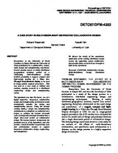
Table 6: BVH build times for one BVH, and for a build over time with 10 candidates, as well as per-frame update time split into triangle update and bounding box refitting. Figure 6: Visualization of the hierarchy for the poser model at frame 14. Left: The full model. Right: The three of the eight level 3 subtrees containing the main body. Top: A deformed BVH originally built for frame 0. Bottom: The best BVH over time. The best tree over time does find the natural partitioning quite well, whereas the deformed first tree did far worse in separating the arms from the body, and has much larger subtrees with significant overlap.

partition based on all known deformations at each recursive partitioning step. Since this function has to evaluate different poses of the model in each partitioning step, this best split over time can be quite expensive. For all the models we tested, the results were usually the same as with the simpler method of constructing a BVH for each time step. Whether there are models that would benefit from the more sophisticated build method is unknown. Note that we are not interested in finding a BVH that is the optimal one for each potential pose of the model, as such an always optimal pose probably does not exist. In contrast, we are looking for the BVH that deteriorates the least over all possible poses.

4.1

Performance on deformable models

Our BVH was implemented in C++, and uses SIMD extensions via SSE intrinsics that are available with both the Intel compiler as well as on recent versions of GCC. The code is mainly optimized for Opteron CPUs, but also runs on Intel processors, and was prototypically implemented on an Apple G5 using Altivec instructions. It does not contain any scene or machine specific code, although choosing between 8 × 8 and 16 × 16 packet sizes was done manually for each model. To illustrate the performance of our system we use three sample animations described later in this section. To establish that our system is fast for static models that are more like typical deformable scenes than the architectural models shown in Table 1, we compared performance with OpenRT on the first frame of each of the animations (Table 7). We now show how these numbers are affected by using a shared BVH topology across time for each of the scenes. These scenes were chosen to highlight different properties of the algorithm, especially robustness of for different types of scenes.

BVH updates. Given a tree whose topology is valid but whose AABB coordinates are not valid for the current frame, we need to quickly update these coordinates. This procedure is straightforward as shown in Algorithm 4. Because we use an ordered traversal, the flag indicating which of the three axes is “dominant” also needs to be updated when the box positions are. The build times running into seconds in Table 6 show why rebuilding the tree for each deformation is impractical. While we could store trees customized for known timesteps, this would increase update time, and more importantly would preclude using our BVH in applications where deformations result from physics or user interaction. The time for building the best BVH over time is then mostly linear in the number of chosen candidate BVHs. For all our experiments, 10-20 candidate BVHs have been sufficient. The times in Table 6 also shows that updating the bounding boxes does not add undue time over updating the triangles.

Runner: a single deformed mesh. We begin with a typical example of a “single model” deformable mesh. It is a 80,000 triangle animated figure from the Poser program and has a reasonable range of deformations. Even for this simple model, deforming a tree built over a fixed timestep can deteriorate quickly: Figure 6 shows the top levels of the BVH from the first frame of animation compared to that using the build over time. Using the better BVH rather than the BVH of the first frame improves performance from 15.3 to 16.2 frames per second. While this improvement is worth attaining given that the build over time is straightforward, its relatively small magnitude surprised us given that the BVH for the first frame looks so much worse. An explanation for the small improvement is that while the packet based traversal does benefit from good trees, it is surprisingly robust when those trees deteriorate incrementally. This is fact is the key to its performance in animation and allows us to use one

Algorithm 4 BVH update after triangles move function UpdateBBoxes(Node node) if node is leaf then bounds(node) ← boundsOf(triangles(node)); else (c0, c1) = children(node); UpdateBBoxes(c0) UpdateBBoxes(c1) node.bounds = ∪{ bounds(c0), bounds(c1) } recompute ordered traversal information end if end

7

Submitted to the 2006 ACM SIGGRAPH conference proceedings 0.45

Worst Per Frame Build over Time Best Per Frame

0.1

Worst Per Frame Build over Time Best Per Frame

0.4

Seconds Per Frame

Seconds Per Frame

0.35 0.08

0.06

0.04

0.3 0.25 0.2 0.15 0.1

0.02

0.05 0

0

5

10

15 Frame Number

20

25

0

0

5

10

15

20

25

Frame Number

Figure 7: The ray tracing times per frame for the Runner model for 16 × 16 ray packet (left), and 4 × 4 ray packets (right). The BVHs used are the same for both graphs and only packet size varies. The blue bars represent the times for each frame when a separate BVH is built for each frame (BVH build time not included). The green shows the times using a shared BVH among all the frames (BVH update time included). The red shows the time when the worst BVH from all other frames is used for each frame (BVH build time not included). Figure 8: Four example frames from the Toys sequence, with the hierarchy visualized via color-coding. The build over time automatically separates the individual objects into individual subtrees. On a single 2.6 GHz Opteron, this scene renders fullscreen at 10.5 fps, including shading, shadows, and animation.

tree over time. The left graph in Figure 7 shows efficiency broken down by frames of the animation. Note that for 16×16 ray packets, our build-over-time method is never more than about 15% slower than using a custom BVH for each frame. More surprising is that if we actively seek the worst BVH to use for each frame, we only are still within about 30% of the times using custom BVHs for each frame. Note that this is a peculiarity of our algorithm, and not true for every BVH traversal method; even for a badly chosen hierarchy, deformations will mostly result in getting some rather large bounding volumes close to the root. In our algorithm, these large volumes will trigger the early hit exit, and thus are extremely cheap to traverse. Evidence for this can be seen in the right of Figure 7 that shows the 2 × 2 ray packet code that does not benefit as much from packet optimizations. Not only does the overall speed slow down about a factor of four, the relative performance of the build-overtime tree jumps from 15% to 40%, presumably because more rays are tested against the larger boxes in the tree. Note that the trees are the same for both cases. There are two additional important factors causing the small deterioration over time. The first is that the SAH build tends to find objects and groups of objects and place them together in subtrees. The second is the ordered traversal employed by our traversal algorithm. During the animation, the deformation to the subtrees can make an originally left subtree move to the right, and the right one move to the left. For example, this happens every time the runner’s legs make a full step. However, each node’s ordered traversal information is recomputed during each BVH update, and will make sure that the traversal order will be correct.

tually simpler to find than for an animated mesh by putting each of the animated objects into a separate subtree. Though this would be trivial and highly efficient if that scene hierarchy were specified explicitly by the application (which in practice is usually the case), the build over time can also find this hierarchy automatically, and without any effort: If a split separates two objects, their boxes over all frames will be small, and the associated cost low; if a split accidentally groups part of one model with a different model, the resulting cost over deformation will be huge, and not accepted. Because the SAH tends to place objects in their own subtrees, the build over time works mostly as expected. However, the first split is somewhat unintuitive in that it first separates the larger ground object. Because the split happens in the middle of the toys it splits each in half. Each of these halves does get its own subtree. This horizontal chopping of all toys could be avoided if our algorithm were allowed to exploit knowledge about the scene hierarchy. While unintuitive, this split is not a bad split from the expected cost perspective, and in fact may be the right one to have taken. The order in which the objects themselves are grouped in the upper levels of the BVH is less obvious if the movement is mostly incoherent. Thus, the BVH’s upper few boxes can become quite large when the objects start to move. However, this only affects the first few bounding volumes close to the root. Since these get traversed extremely quickly by the “first hit” optimization, this is probably not expensive. Thus, even in this example we achieve a performance of 10.5 frames per second (on average) on a single Opteron 2.6 GHz CPU (at 1024x1024 pixel) including shading and shadows. The impact of using a built-over-time BVH for all frames is, like for the Runner scene, relatively small (Figure 9, left).

Toys: incoherent motion of individual objects. The previous example has shown that a BVH can be shared for deformations of an individual objects. However, typical interactive applications use multiple animated objects at the same time. These usually show a totally different dynamic behavior: they run around each other, are sometimes close and sometimes far apart from each other, etc. Such a scene is shown in Figure 8, where a set of animated wind-up toys run incoherently around among each other, bump into each other, and even jump over each other. Since this kind of motion is completely different from a single deformed mesh, it is not obvious that our method can handle it as well. However, our method does not depend on a single, connected mesh, but only on a “natural hierarchy” inherent in the scene. For scenes composed of multiple animated models, this hierarchy is ac-

Fairy-forest: a scene with moving deformable objects. Finally, to stress test our approach with a real-world animated scene, we have taken a free modeling program by DAZStudio, and have created a scene composed of a total of nearly 180,000 animated triangles (Figure 10). The scene consists of an animated 80,000 triangle fairy model dancing through a forest made up of trees and animated ferns. Additionally, a dragonfly – with skinned body and flapping wings - flies around the fairy. The scene also

8

Submitted to the 2006 ACM SIGGRAPH conference proceedings 0.06

Worst Per Frame Build over Time Best Per Frame

Our approach combines ordered traversal, packet traversal, SIMD computations, early BVH hits, and MLRTA-style early exits. This combination turns out to be so natural that the full implementation including all these concepts can be written up compactly.

Worst Per Frame Build over Time Best Per Frame

0.25

0.05 Seconds Per Frame

Seconds Per Frame

0.2 0.04

0.03

0.02

Limitations. There are several limitations to our current approach. It is limited to deformable scenes, so only triangle positions can be changed. Thus applications with primitives such as adaptive meshes or particle systems with births and deaths could be a problem. Because we assume some reasonably smooth space of poses, our BVH might not be efficient for some models. So far, however, we have not found an animation sequence that exhibits this behavior. Finally, even for scenes composed of multiple objects we currently assume that all these objects are known in advance, and that their positions can be sampled. In practice, however, many interactive applications consist of several independent models that are moving incoherently, and no advance knowledge at all of how many of these models will be in the scene, nor where these will be, at any time. In that case the upper levels of the hierarchy that group the scene’s individual objects would have to be rebuilt. Though we believe this is feasible, a concrete demonstration would need to be created before we could conclude that.

0.1

0.05

0.01

0

0.15

0

5

10 Frame Number

15

20

0

0

5

10

15

20

Frame Number

Figure 9: Left: performance of 20 frames from the 250 frame Toys scene with 16 × 16 ray packets. As with the Runner scene, there is little overhead added by sharing a BVH between frames. Right: the same measurements for the Fairy scene.

Figure 10: Fairy-forest test scene: An animated dragonfly (a) and a dancing fairy (b), placed into a typical game environment with background textures and animated foreground geometry (c). The resulting scene (d) consists of 180,000 animated triangles, and is rendered with textures, shading, and shadows, at 2.2 fps at 1024 2 resolution.

Future work. To help compare different approaches, the ray tracing community needs a set of animation benchmarks similar in spirit to the static SPD database developed by Haines [1987]. There is some movement in this direction [Lext et al. 2000] but more is needed. To address the limitation to deformable scenes, incremental trees that can change the number of leaves is worth investigating. To make the BVH more general, oriented bounding primitives could be helpful. There are several optimizations that could improve our run times. First, there are algorithmic techniques such as marking shadow rays once they are occluded to prevent redundant traversal and intersection, exiting once all shadow rays are occluded [Smits 1998], and the same optimizations for architectural scenes that are being used in MLRTA [Reshetov et al. 2005]. Second, there is considerable room for low-level optimizations. Although we already use SIMD extensions, most of the code is written for flexibility, simplicity, and portability, and makes use of templated high-level C++ code. We believe there is potential in further optimizing this code if more aggressive and architecture-specific coding were performed. Finally, our algorithm could benefit from powerful hardware architectures such as IBM’s Cell processor [Minor et al. 2005]. If our algorithm maps well to the Cell, which we believe it will, it could run at 10x the speeds reported here and ray tracing on commodity game consoles might finally come into reach. Finally, adapting our system to interactive modeling applications would be the ultimate test of whether ray tracing could become an everyday interactive technique.

makes use of textures (30 megabytes total), and – though the background and floor textures are pre-lit – is rendered with shadows from a point light source. This scene intentionally stresses several issues for our approach: It is quite complex, and with 180,000 triangles in the complexity range of today’s games; it is almost fully animated, but no knowledge about the modeling hierarchy is provided to our algorithm (except some sample frames); the surrounding geometry with tall trees and background objects stresses some “teapot in a stadium” situations and makes hierarchy construction non-obvious. Our algorithm handles this scene surprisingly well. Without shading and shadows – but with full animation – the five example frames in Figure 1 render at 6.0 – 6.5 frames per second on a single CPU. This includes the time to recompute all of the 180,000 triangles and 100,000 vertices every frame, as well as the time to recompute bounding volumes and the triangle acceleration structure required for the triangle test (Figure 9, right). Including shading and shadows, the performance drops considerably as expected. As reported by [Reshetov et al. 2005], for a fast ray tracer even a simple shader computing only a dot product can reduce performance by 50%. Additionally, our shader interpolates shading normals, computes textures coordinates, touches megabytes of textures, and shoots shadow rays. Nevertheless, we still achieve 2.0 to 2.3 frames per second on a single CPU, and 3.4 to 4.0 frames per second once we enable the second CPU in our PC.

References A DAMS , B., K EISER , R., PAULY, M., G UIBAS , L. J., G ROSS , M., AND D UTR E´ , P. 2005. Efficient raytracing of deforming point-sampled surfaces. Computer Graphics Forum 24, 3 (Sept.), 677–684. A DELSON , S. J., AND H ODGES , L. F. 1995. Generating exact ray-traced animation frames by reprojection. IEEE CG&A 15, 3, 43–52.

5 Conclusion

A PPEL , A. 1968. Some techniques for shading machine renderings of solids. SJCC, 27–45.

In this paper, we have presented two main contributions: a novel ray packet traversal scheme for BVHs, and a method for BVH construction that allows many deformations of the same scene to reuse the same hierarchy. Taken together, these two techniques allow for ray tracing animated models at a performance that is competitive to the fastest ray published ray tracing performance for static models.

A RVO , J., AND K IRK , D. 1989. A survey of ray tracing acceleration techniques. In An Introduction to Ray Tracing, A. S. Glassner, Ed. Academic Press, San Diego, CA. B ENTLEY, J. L. 1975. Multidimensional binary search trees used for associative searching. Communications of the ACM 18, 9, 509–517.

9

Submitted to the 2006 ACM SIGGRAPH conference proceedings C ARR , N., H OBEROCK , J., C RANEH , K., AND H ART, J. 2006. Fast GPU ray tracing of dynamic meshes using geometry images. In Proceedings of Graphics Interface (submitted).

¨ M ULLER , G., AND F ELLNER , D. 1999. Hybrid scene structuring with application to ray tracing. In Proceedings of International Conference on Visual Computing, 19–26.

C LARK , J. H. 1976. Hierarchical geometric models for visible surface algorithms. Communications of the ACM 19, 10, 547–554.

M UUSS , M. 1995. Towards real-time ray-tracing of combinatorial solid geometric models. In Proceedings of BRL-CAD Symposium.

C LEARY, J., W YVILL , B., B IRTWISTLE , G., AND VATTI , R. 1983. A Parallel Ray Tracing Computer. In Proceedings of the Association of Simula Users Conference, 77–80.

N G , K., AND T RIFONOV, B. 2003. Automatic bounding volume hierarchy generation using stochastic search methods. In Mini-Workshop on Stochastic Search Algorithms.

C ROSS , R. A. 1995. Interactive realism for visualization using ray tracing. In Proceedings of Visualization, 19–26.

PARKER , S. G., M ARTIN , W., S LOAN , P.-P. J., S HIRLEY, P., S MITS , B. E., AND H ANSEN , C. D. 1999. Interactive ray tracing. In Proceedings of Interactive 3D Graphics, 119–126.

F OLEY, T., AND S UGERMAN , J. 2005. Kd-tree acceleration structures for a gpu raytracer. In Proceedings of HWWS, 15–22.

PARKER , S. 2002. Interactive ray tracing on a supercomputer. In In Practical Parallel Rendering, A. Chalmers and E. Reinhard, Eds.

G LASSNER , A. S. 1984. Space subdivision for fast ray tracing. IEEE CG&A 4, 10, 15–22.

P URCELL , T., B UCK , I., M ARK , W., AND H ANRAHAN , P. 2002. Ray tracing on programmable graphics hardware. In Proceedings of SIGGRAPH, 703–712.

G LASSNER , A. 1988. Spacetime ray tracing for animation. IEEE CG&A 8, 2, 60–70. G OLDSMITH , J., AND S ALMON , J. 1987. Automatic creation of object hierarchies for ray tracing. IEEE CG&A 7, 5, 14–20.

R EINHARD , E., S MITS , B., AND H ANSEN , C. 2000. Dynamic acceleration structures for interactive ray tracing. In Proceedings of the Eurographics Workshop on Rendering, 299–306.

¨ G R OLLER , E., AND P URGATHOFER , W. 1991. Using temporal and spatial coherence for accelerating the calculation of animation sequences. In Proceedings of Eurographics, 103–113.

R ESHETOV, A., S OUPIKOV, A., AND H URLEY, J. 2005. Multi-level ray tracing algorithm. In (Proceedings of SIGGRAPH, 1176–1185. RUBIN , S., AND W HITTED , T. 1980. A 3D representation for fast rendering of complex scenes. In Proceedings of SIGGRAPH, 110–116.

G UTTMAN , A. 1984. R-trees: A dynamic index structure for spatial searching. In Proceedings of SIGMOD, 47–57.

S CHMIDL , H., WALKER , N., AND L IN , M. 2004. CAB: Fast update of OBB trees for coll. det. between articulated bodies. JGT 9, 2, 1–9.

H AINES , E. 1987. A proposal for standard graphics environments. IEEE CG&A 7, 11, 3–5.

S MITS , B. 1998. Efficiency issues for ray tracing. Journal of Graphics Tools 3, 2, 1–14.

H AINES , E. 1991. Efficiency improvements for hierarchy traversal in ray tracing. In Graphics Gems II, J. Arvo, Ed. Academic Press, 267–272.

B ERGEN , G. 1997. Efficient collision detection of complex deformable models using AABB trees. JGT 2, 4, 1–14.

VAN DEN

H AVRAN , V. 2001. Heuristic Ray Shooting Algorithms. PhD thesis, Faculty of Electrical Engineering, Czech Technical University in Prague.

WALD , I., S LUSALLEK , P., B ENTHIN , C., AND WAGNER , M. 2001. Interactive rendering with coherent ray tracing. In Proceedings of Eurographics, 153–164.

H URLEY, J. T., K APUSTIN , A., R ESHETOV, A., AND S OUPIKOV, A. 2002. Fast ray tracing for modern general purpose CPU. In Proceedings of GraphiCon.

WALD , I., B ENTHIN , C., AND S LUSALLEK , P. 2003. Distributed interactive ray tracing of dynamic scenes. In Proceedings of PVG, 77–86.

JANSEN , F. 1986. Data structures for ray tracing,. In Proceedings of the Workshop in Data structures for Raster Graphics, 57–73.

WALD , I. 2004. Realtime Ray Tracing and Interactive Global Illumination. PhD thesis, Saarland University.

K APLAN , M. 1985. The uses of spatial coherence in ray tracing. In ACM SIGGRAPH ’85 Course Notes 11.

W EGHORST, H., H OOPER , G., AND G REENBERG , D. 1984. Improved computational methods for ray tracing. ACM TOG 3, 1, 52–69.

K AY, T., AND K AJIYA , J. 1986. Ray tracing complex scenes. In Proceedings of SIGGRAPH, 269–278.

W HITTED , T. 1980. An improved illumination model for shaded display. CACM 23, 6, 343–349.

K IRK , D., AND A RVO , J. 1988. The ray tracing kernel. In Proceedings of Ausgraph, 75–82.

W ILLIAMS , A., BARRUS , S., M ORLEY, R. K., AND S HIRLEY, P. 2005. An efficient and robust ray-box intersection algorithm. JGT 10, 1, 49–54.

¨ L ARSSON , T., AND A KENINE -M OLLER , T. 2003. Strategies for bounding volume hierarchy updates for ray tracing of deformable models. Tech. Rep. MDH-MRTC-92/2003-1-SE, MRTC, February.

W OOP, S., S CHMITTLER , J., AND S LUSALLEK , P. 2005. RPU: A programmable ray processing unit for realtime ray tracing. In Proceedings of SIGGRAPH, 434–444.

¨ L ARSSON , T., AND A KENINE -M OLLER , T. 2005. A dynamic bounding volume hierarchy for generalized collision detection. In Workshop On Virtual Reality Interaction and Physical Simulation, 91–100. ¨ L EXT, J., AND A KENINE -M OLLER , T. 2001. Towards Rapid Reconstruction for Animated Ray Tracing. In Proc. of Eurographics, 311–318. ¨ L EXT, J., A SSARSSON , U., AND M OLLER , T. 2000. BART: A benchmark for animated ray tracing. Tech. rep., Department of Computer Engineering, Chalmers University of Technology, Go¨ teborg, Sweden, May. M AC D ONALD , J. D., AND B OOTH , K. S. 1989. Heuristics for ray tracing using space subdivision. In Proceedings of Graphics Interface, 152–63. M AHOVSKY, J., AND W YVILL , B. 2004. Fast ray-axis aligned bounding box overlap tests with Pl¨ucker coordinates. JGT 9, 1, 35–46. M AHOVSKY, J. 2005. Ray Tracing with Reduced-Precision Bounding Volume Hierarchies. PhD thesis, University of Calgary. M ARK , W., AND F USSELL , D. 2005. Real-time rendering systems in 2010. Tech. Rep. 05-18, Computer Science, University of Texas, May. M INOR , B., F OSSUM , G., AND T O , V. 2005. TRE : Cell broadband optimized real-time ray-caster. In Proceedings of GPSx. ¨ M OLLER , T., AND T RUMBORE , B. 1997. Fast, minimum storage ray triangle intersection. JGT 2, 1, 21–28.

10