Flight Critical Systems, Line Replaceable Unit , Integrated Modular Avionics, Time ... The avionics systems and software architecture of federated era was no ...
ISBN: 978-972-8924-39-3 © 2007 IADIS
RE-CONFIGURABLE AVIONICS ARCHITECTURE ALGORITHM FOR EMBEDDED APPLICATIONS CM Ananda, Aerospace Electronics & Systems Division, National Aerospace Laboratories, Bangalore, India
ABSTRACT The paper presents a new method for re-configuration of tasks or a process in an embedded avionics application. The proposed algorithm works based on four control parameters: re-configurability Information factor, Schedulability Test/TL/UF, Context Adaptability/suitability and Context Flight Safety. The algorithm is data centric and interfaces system health as control input and initiation of the re-configuration is only after successful evaluation of the parameter metrics. It enhances the availability and reliability of the system under failed conditions by efficient selection and procedural re-configuration with safe state exit. The advantage of the new approach over the non-configurable systems is the increased availability of flight critical applications under failed conditions. It also preserves the advantages of nonReconfigurable systems over federated architecture. Invalid failure of control parameter brings the system to safe state. The scheme, algorithm and the control parameters metrics and their validation approach are described. The algorithm is novel in terms of dynamic re-configuration compared to existing static avionics architecture KEYWORDS Flight Critical Systems, Line Replaceable Unit , Integrated Modular Avionics, Time Loading, major frame, Availability
1. INTRODUCTION The avionics systems and software architecture of federated era was no doubt very good in terms of the fault containment, fault tolerant and a sort of fool proof architecture. However, this has disadvantages like, increased weight, redundant computer resources in each Line Replaceable Unit(LRU), higher looming volume, electrical interfaces complexity and physical maintenance. The advances in computer technology encouraged the avionics industry to utilize the increased processing and communication power and combine multiple federated applications into a single shared platform [1]. The Integrated Modular Avionics (IMA) was developed for integrating multiple software components into a shared computing environment[1a]. This is powerful enough to meet the computing demands of multiple applications using common hardware and system resources. The IMA integration has the advantage of lower hardware costs and reduced level of spares Related work and Motivation Existing mechanism of system behavior in the event of a task failure is to declare system failure resulting in non-availability either by part or full partition functionality. Here the failure recovery by removing the faulty task or replacing by a new task is not exercised. However, all the failures cannot be re-configured due to the safety and criticality of the avionics applications. The novelty of the proposed algorithm is of reconfiguring the critical tasks or removal from the schedule to enable continued functionality of the non-faulty partition using control metrics [2]. This aspect has motivated to propose a new approach of re-configuration to attain higher system availability and improved reliability. This paper focuses on the re-configuration algorithm; rule based decision-making approach and control metrics coupled with state and condition matrix. The algorithm is described for a typical multi partitioned multiple process task based architecture.
154
IADIS International Conference Intelligent Systems and Agents 2007
2. ORGANIZATION OF TASK OR PROCESS SCHEDULER IN A TYPICAL AEROSPACE AVIONICS APPLICATION Typical aerospace applications employ multiple functionalities with the same hardware and system software. This uses the concept of major frames, multiple partitions and each partition having multiple processes to schedule the tasks. Figure 1 shows the set of partitions [3], which are scheduled across a major frame M consisting set of partitions …(1)
M = {Pt1 , Pt 2 .........Pt n }
P1 P2 P3 P4
P1 P2 P3 P4
…..
P11 P22 P33 P44
Cip
Tip
Tip Major Frame period Figure 1. Static table schedule diagram with partition period and process execution duration
Consider a major frame M having a set of partitions Pti..Ptn based on functionalities. Each partition Pti consists of a set of process Psi…Psn based on the applications sub functionalities. The number of partitions and number of processes in each partition is a trade-off to get the real time response based on the capabilities of the hardware and software together. The representation of Major frames and processes is ⎡ Pt ⎤ ⎢ 1⎥ ⎢ ⎥ ⎢Pt 2 ⎥ ⎢ ⎥ Major Frame= ⎢Pt3 ⎥ ⎢ ⎥ ⎢ . ⎥ ⎢ ⎥ ⎢ ⎥ ⎢⎣Pt n ⎥⎦
=
⎡ Ps ⎢ 11 ⎢ ⎢ Ps21 ⎢ ⎢ Ps 31 ⎢ ⎢ . ⎢ ⎢ ⎢⎣ Psm1
Ps12 Ps13 Ps22 Ps23 Ps32 Ps33 . . Psm2 Psm3
. . . . .
Ps1n ⎤⎥ Ps2n ⎥⎥ ⎥ Ps3n ⎥ = ⎥ . ⎥⎥ Psmn ⎥⎥⎦
⎡τ ,τ ,....τ n ⎢ 1 2 ⎢τ ,τ ,....τ ⎢ 1 2 n ⎢ ⎢τ 1 ,τ 2 ,....τ n ⎢ ⎢ ⎢ ⎢τ ,τ ,....τ n ⎣⎢ 1 2
τ 1 ,τ 2 ,....τ n τ 1 ,τ 2 ,....τ n τ 1 ,τ 2 ,....τ n τ 1 ,τ 2 ,....τ n
τ 1 ,τ 2 ,....τ n ⎤ ⎥ τ 1 ,τ 2 ,....τ n ⎥⎥ ⎥ ,....τ ⎥ τ 1 ,τ…(2) 2 n ⎥ ⎥ ⎥ τ 1 ,τ 2 ,....τ n ⎥⎦⎥
…(2) Each process Ps consists of set of tasks τ1 .. τn and the sequence of tasks are predefined and priorities are fixed as per static table scheduling mechanism and each task τI has definite timing characteristics: Ci ≤ Di ≤ Ti, where Ci - Task Worst Case Execution Time , Di - Task Deadline and Ti - Period Also each task τI has other timing characteristics, which are critically examined for real-time capabilities like Worst Case blocking, Worst Case partition Delay, Worst Case Process Jitter and OS overheads. During the execution of a process, Worst Case Execution Time ( WCET) and Worst Case process Jitter ( J ) are the two important timing characteristics to be considered for realistic estimation of execution time. Worst Case Process Jitter ( J ) quantifies the maximum difference of the response time with the execution times for each period [4]. Jitter depends on the Kernel overheads and partition jitter. Typical jitter measurements were carried out using embedded target to study the jitter timings( refer 3.4 ). These timing measurements help to characterize the delays and execution non-linearity in the algorithm. However the response time of a task τI or Process Pi encompasses the various delays and execution times and they are Where Li – Interrupt latency time, Cs – Context save time, Si – Schedule time, Ai – Process Time Li Ai C s Si Therefore the response time is expressed as Ri = Li + Cs nS mS µS µS + Si + A i
155
ISBN: 978-972-8924-39-3 © 2007 IADIS
3. PROPOSED ALGORITHM 3.1 Control parameters for the proposed algorithm A new re-configuration algorithm using critical control parameters is introduced using control parameter metrics. The re-configuration algorithm is implemented based on four major metrics, which are the heart of the algorithm in re-configuration. The Re-configurability Information-Factor, Schedulability Test/TL/UF, Context Adaptability/suitability and Context Flight Safety Factor are the efficient decision making control parameters defined and used in the algorithm. Based on these control metrics, the re-configuration GO/NOGO is decided. A. Re-configurability Information-Factor (RI) :Re-configurability Information Factor (RI) is defined as the ratio of re-scheduled Task or Process Functional Credit Point (FCP) to the original scheduled task or process FCP. The FCP is the measure of the functionality characteristics in terms of its requirement and weight-age of the task or process to accomplish the defined system accomplishments and are derived from the system requirements, design limits and Failure Mode Effect Analysis and Testing guidelines. For every selected critical task (τs) in a Major frame consisting of number of scheduled lists, there can be at least one configurable task (τr). The selection of replaceable task is based on the RI i.e., a process Ps or task τs can be re-configured by a process Pr or a task τr if and only if the RI of new process Pr or task τr should be at least equal to or greater than the RI of the faulty process Ps or task τs and is expressed as …(3) (τ = τ ) ← ⎯→ ( RI(τ ) ≥ RI(τ ))or ( P = P ) ← ⎯→( RI(P ) ≥ RI(P )) s
r
s
r
s
r
s
r
FCP is derived based on the type of task, criticality of the task and phase of application envelope. For all critical tasks task τ in a process Ps scheduled in a partition Pt, has a defined FCP. B. Schedulability Test (Time Loading TL or Utilization Factor UF): Schedulability Test is the standard method of testing the time loading or utilization for a task to be scheduled ⎛ s C s t Ct ⎞ and ⎜ (∑ (τ s = τ t ) ← ⎯→ WCET(τ ) ≤ WCET(τ ) ( τ τ ) )⎟ = ← ⎯→ ≤ s t s t ⎜ i =1 Ts i∑ ⎟ …(4) =1 Tt
(
)
n
⎝
i
i
n
i
i
⎠
Similarly for a process, the faulty process shall be replaceable if and only if …(5) ⎛ sn As 2n A2 ⎞ ⎯→ WCET(P ) ≤ WCET(P ) and ( Ps = P2 ) ← s 2 ( Ps = P2 ) ← ⎯→⎜ ∑ i ≤ ∑ i ⎟ ⎜ i =1 Ts i =1 T2 ⎟ n C i i ⎠ ⎝ n ∑ i ≤ U (n) = n(2 − 1) T For all cases of task phasing, a set of n tasks will always meet their deadlines [4] ifi =1 i ≤ 0.69 …(6) and this is strictly enforced in algorithm for static computation of time loading in each schedule table of every partition. Execution time or utilization is the important data resulting in efficient selection of a task or process to reconfigure. Each task is benchmarked with the execution times and the same is used in real time for the algorithm and the corresponding matrix also updated for use by the algorithm. For the selected critical tasks, reference execution time dataset is compiled and generated in accordance with (2). The algorithm checks this reference dataset for task selection criteria. C. Context Adaptability and Suitability ( CAS ): Context Adaptability and Suitability metric decides acceptability of the faulty task replacement in real time. This involves checking the state table and condition table to decide whether the re-configuration is permissible. Hence the context of the scenario is verified and validated for the functionality and context suitability of the task. Context Adaptability and Suitability (CAS) is defined as …(7) ( CAS = TRUE ) ← ⎯→ ( re − scheduled Task or process Context flag AND ) == T
(
)
Original Task or process Context
flag
Every task in a process and partition has the CAS flag dictating the function’s use at that point of time using task reference dataset condition table. However, each task can have more than one suitable tasks depending on the prevailing scenario (P- phase of flight ) in real time. This aspect is very important and has not been explored. The CAS condition table used in the algorithm is derived based on the system functionality and inter system re-configuration dependencies.
156
IADIS International Conference Intelligent Systems and Agents 2007
D. Context Flight Safety Factor (CFS) : It is very vital in aerospace flight critical applications to check the safety of the system before and after re-configuration. After validating the above three control parameters, the system is checked for safe state to initiate re-configuration. For aircraft systems in closed loop control, a wrong function being re-configured can lead to catastrophic failure. Hence any action carried out in real time is verified and validated thoroughly by all the control parameter artifacts along with the system information. Context Flight Safety Factor (CFS) is defined as re − scheduled Task or process SafetyFactor ( original ) scheduled Task or process SafetyFactor
(CFS = TRUE) ←⎯→
…(8)
≥ 1.0 A process Ps or task τs can be re-configured by a process Pr or a task τr if and only if the safety factor of new process Pr or task τr should be at least equal to or greater than the safety factor of the faulty process Ps or task τs and is expressed as …(9)
(
)
( P = P ) ←⎯→ CFS ( P ) ≥ CFS ( P ) , s r s r
(τ
s
(
= τ ) ←⎯→ CFS (τ ) ≥ CFS (τ ) r s r
)
CFS is derived from both RI and the safety units (Su) based on the Failure hazard Analysis (FHA), Failure Mode Effect Analysis ( FMEA ) and System Safety Analysis (SSA)[5]. The final safety unit being used by the algorithm is part of the CFS matrix. The Degradation Factor(DF) is the measure of allowed degraded performance or functionality in selected envelope of the system being re-configured. This degraded functionality is carefully studied and defined. If degraded functionality is not allowed then the degradation factor is 1. Input reference dataset for the control parameters used in the algorithm depends on the information of the system are captured by System Design/ analysis, Sample Implementation on typical platform, Aircraft Level Failure Hazard Analysis (FHA), System level Failure Mode Effect Analysis ( FMEA), FAA/TSO requirements for aerospace flight critical systems and System Safety Analysis (SSA)
3.2 Condition, status and state information:
3.3 Re-Configurable Algorithm: A non-Reconfigurable system either shuts down or performs a partial degraded functionality in the event of a task failure. In some cases, this may lead to infinite loops or crash of the application leading to serious failure. Here the fault is not resolved rather the system enters failed state.The proposed algorithm overcomes above fault scenario by re-configuration of faulty task resulting in recovery of fault in complete or partial. The algorithm replaces a faulty process or task by a compatible, suitable and safe substitute after extensive check and validation. The re-configured task or process performs the required operation without any safety impact to the system and aircraft. After careful design and definition of control parameter metrics for re-configurable decision-making as described in section 3.1, the following algorithm is proposed for re-configuration of a task or a process. The algorithm has the fail off path in case the algorithm enters the fault loop with multiple re-configurations without effective output. This is handled by a re-configuration counter, which avoids the repetitive reconfiguration for the same failure. Proposed Algorithm • If a task/job fails • Capture the task( τs ) status, functionality, priority, criticality to identify the faulty task • Identify the most suitable substitution task( τr ) after validating the control metrics( Sec 3.1 A, B, C and D) for feasibility • If re-configured task fails, • If the system can run in de-graded mode • Revert all tasks to its original state • Identify set of tasks which needs to be removed from the schedule • re-schedule the task set with de-graded performance using dead task removal techniques ( all the failed tasks are removed from the task set ) • The rest of the task set continues to run provided no safety impact after re-schedule • In case de-graded mode is not feasible, • Declare failure and enter the fail state of the system
157
ISBN: 978-972-8924-39-3 © 2007 IADIS
The algorithm plays the role of high-level real time monitor software continuously monitoring the status of the running tasks of a schedule table. The algorithm is explained in the following five phase. Phase I : Status Capture: The algorithm starts with continuous monitoring the status and health of a task execution. The data capture is part of the application software and the algorithm receives the information on function call or through global shared resources. When the algorithm detects a task failure or not performing as per its functionality, then the algorithm initiates the Phase II execution. Phase II : Control parameter validation : The main objective of phase II is to identify the most suitable task using the results of control parameter validations. In any case, if any of the control parameter fails to comply with limit values, the algorithm returns to the system without any action resulting in resumption to the original state or transits to phase IV. Because of the extensive validation process using four control parameters, the probability of phase II passing is quite high. On successful completion of control parameter checking and validation, the algorithm initiates the Phase III execution. Phase III : Re-configuration: During the re-configuration process, the global state of the system, process or partition is not altered. Only the selected task or process gets altered for their respective state variables. On successful re-configuration, the re-configured task start execution in the next major frame. Phase IV : De-graded performance: If the re-configured task fails again in the next major frame, then the algorithm reverts back to its earlier state by reverting the re-configured task. If the degraded performance or functionality is allowed for that particular function, then the algorithm removes the faulty task or process from the schedule table and allows it to continue. In this case, the system continues to execute without the functionality of removed task. This is still an improved mechanism instead of totally shutting down the application with many others tasks in good state. Phase V : Fail off procedure: During the execution of the algorithm if the degraded functionality is not allowed then the algorithm behaves similar to the normal process of entering failed state. The re-configuration algorithm is applied only for the critical task or process, which improves the availability as an effect of re-configuration. The algorithm is simulated on a test platform using predefined known states and the work is in progress to simulate using the realistic dataset. The simulated results under defined conditions shows significant improvement from reliability numbers from 1E-05 to 1E-07 under failed conditions for critical task. Configuration of a task or a process in aerospace flight critical system is a crucial event with the safety of the aircraft and availability of systems. Hence to identify a task for re-configuration requires severe judgment, methodical analysis, extensive cross checking across various relative parameters in real-time. The control parameters are checked for their states, status and validation before re-scheduling the sequence of tasks. Failure data collection for various scenarios is based on standards and equipment life cycle and quality control data management[6]
3.4 Simulation and Experimental Data A sample schedule partition is simulated in Matlab Simulink using the state machines to check the time loading and execution scenarios. Even though the target is not that of a real environment, this gives a platform to study the timing behavior of system under varying external reactive interfaces. Experiments using low scale target hardware shows an average of ± 0.1 ms, ±0.14 ms, ± 0.2 and ±0.2 ms execution and jitter timing for 10,30, 40 and 50 ms interrupt intervals for various configurations under multiple code composition in terms of the control and data flow deviations. The scenarios were simulated to capture the worst-case timings with constructs simulating the single and multiple failures. The measurements were carried out with an embedded target system working at 20.0 Mhz clock and Fs/4 internal clock frequency. Measurements show an average value of 20 to 30 microSec for the interrupt jitter or interrupt arrival interval time. However these numbers vary across target to target with different clock frequencies and architectures. In this experiment an effort was made to study the interrupt interval time variation with varying clock frequencies and dynamic external reactive inputs for the same target. Context switching time is very vital in determining the response time of a task. An effort was made to capture typical switch time between an interrupt and a task entry / exit-using RISC based Micro-controller as target. These measurements will be used for algorithm simulation. Experiments also showed the interrupt and function call timing issues in entry and exit conditions based on simulated task execution is 2.52 and 7.62 µsec for 11.056 MHz and 4.0 MHz clock respectively. The complete partition schedule was simulated using Matlab Simulink and the time loading aspects were studied
158
IADIS International Conference Intelligent Systems and Agents 2007
with varying time loading or utilization of 0.32 to 0.7. Also simulation was done with varying fault scenarios and the results of varying task timings are as shown in Figure 2 and Table 1. The tasks used in the simulation were first scheduled as per the fixed priority scheduler and the sequence of tasks and its execution times were simulated using Time Optimization of Resources, SCHEduling (Torsche) toolbox[7]. Torsche results were used to sequence the tasks in Matlab Simulink as table driven fixed priority scheduling for implementing the algorithm. Trail #1(ms) 4.77 IO Proc 3.33 Sensor Valid 0.03 LMS Filter 1.27 Cross Comp 3.9 RT Comp 3.9 Data Format 0.03 Output Proc 0.03 Fault Mngt TL(%) 69.17 Tasks
Figure 2. Simulation of multiprocessor multi task schedule table using Matlab Simulink with varying fault scenarios.
Trail Trail Trail Trail #2(ms) #3(ms) #4(ms) #5(ms) 4.57 3.23 0.03 1.25 2.86 4.10 0.03 0.03 64.50
3.50 4.44 0.032 1.26 3.90 3.50 0.034 0.031 66.88
4.64 3.12 0.031 1.28 3.86 2.66 0.031 0.032 62.73
4.11 3.46 0.034 1.29 3.75 2.54 0.030 0.031 61.06
Table .1 Timing for a varying fault scenario of a set of tasks
4. CONCLUSION AND FUTURE WORK Consequent to intense research and study, the algorithm along with the control parameter metrics were designed and defined. Identification of suitable task as a substitute for a faulty task is very crucial and difficult task. The effectiveness of the algorithm is purely dependent on the system information available at the instance of failure in real time. Also the fault models of the dynamic environment should be considered for simulation for a realistic behavior of the algorithm. The simulation is being carried out using True Time[8] plug-in to Matlab Simulink with various fault scenarios. However the data generation for the control parameter metrics is very crucial for the full-fledged algorithm simulation. The data generation activity is in progress. The solution to the problem of software complexity is not to avoid complexity rather to develop reliable protection and safety mechanisms to handle such scenarios. At the same time the implementation overheads should be maintained to the least possible for effective resource management. The re-configurable algorithm described offers the benefits of higher availability with the state of the art techniques. The algorithm uses reconfigurability Information factor, Schedulability Test/TL/UF, Context Adaptability/suitability and Context Flight Safety for efficient and safe re-configuration for effective failure handling. Bench marking of all these control parameter reference dataset is not covered in this paper. Work is being done in optimization of the control parameter validation process for task selection and compiling the required reference dataset for the algorithm using flight critical open architecture platform. Also the algorithm fault scenarios are being modeled and studied using true time, Torsche and neural network model using Matlab Simulink.
ACKNOWLEDGMENT Author thanks Dr. SV Narasimhan, Deputy Director, National Aerospace Laboratories for his guidance and motivation from time to time. Author also thanks Prof. Y Narahari, CSA IISC, Prof. S Govindarajan, SCRC, IISC, Dr. BS Adiga, Dr.MR Nayak(Head ALD) and Dr. AR Upadhya (Director NAL).
159
ISBN: 978-972-8924-39-3 © 2007 IADIS
REFERENCES [1] ARINC report 651, November 1991, Design Guide for Integrated Modular Avionics, Published by Aeronautical Radio Inc., Annapolis, MD,. [1a] ARINC Specification 653-1, October 2003, Avionics Application Software Standard Interface, Published by Aeronautical Radio Inc., [2] CM Ananda, May 2007, Avionics for general aviation light transport aircraft: An insight into the avionics architecture and integration , AIAA Southern California Aerospace Systems and Technology Conference , Santa Anna, California, USA [3] Neil Audsley and Andy Wellings, 1996, Analyzing APEX Applications, IEEE Real Time Systems Symposium RTSS [4] Loic P Briand and Daniel M Roy, 1999, Meeting deadlines in Hard Real-Time Systems The Rate Monotonic Approach, IEEE Computer Society [5] IEC 60812, 1985,Analysis techniques for system reliability - Procedure for failure mode and effects analysis (FMEA), IEC 60812 Ed. 1.0 b:1985 [6] BS Dhillon,1999, Design Reliability: Fundamentals and Applications, CRC London New York Washington D.C [7] Stibor Miloslav, Kutil Michal, June 13 – 16, 2006, Torsche scheduling toolbox: listScheduling, 7th International Scientific – Technical Conference – PROCESS CONTROL 2006, Kouty nad Desnou, Czech Republic
[8]
Hector Benitez-Perez and Fabian Garcia-Nocetti, 2005, Re-configurable Distributed Control, Springer-Verlag London Limited
160