Real-Time Continuous Collision Detection for Moving ... - CiteSeerX

HKU CS Tech Report TR-2006-02

Real-Time Continuous Collision Detection for Moving Ellipsoids under Affine Deformation §

Yi-King Choi

†

§

Jung-Woo Chang ‡

Wenping Wang

†

Myung-Soo Kim

Gershon Elber

§

†

Dept. of Computer Science, The University of Hong Kong, Hong Kong School of Computer Science and Eng., Seoul National University, South Korea ‡ Dept. of Computer Science, Technion, Israel

Abstract We present an exact algebraic algorithm for real-time continuous collision detection (CCD) for moving ellipsoids under affine deformations. An efficient collision test is first developed for two static ellipsoids, which takes less than 1 microsecond. Using this practical result and the properties of our algebraic condition, we produce a real-time solution to the CCD problem that computes the exact collision time intervals.

keywords: Ellipsoid, motion, deformation, affine transformation, algebraic condition, continuous collision detection, exact algorithm, real-time, independent motion.

1 Introduction Real-time collision detection is crucial to the development of physics engines for 3D computer games [3, 4]. Spheres [7], axis-aligned bounding boxes [6, 16], oriented bounding boxes [5], and discrete oriented polytopes [10] have been successfully used in constructing bounding volume hierarchies and speeding up collision detection among moving 3D objects of complex but rigid shapes. With the proliferation of powerful vertex shaders to commodity graphics cards, recent releases of 3D games demonstrate dramatic shape deformations of 3D characters. Conventional techniques are rather inefficient in reconstructing bounding volume hierarchies under dynamic shape deformations: under affine transformation of

Figure 1: Real-time continuous collision detection in a boxing game.

1

the underlying geometry, there is no guarantee that conventional bounding volumes deform to different bounding volumes of the same type. In this paper, we propose the ellipsoid as an ideal bounding volume for this purpose. In recent work, [12, 13, 14] address the important issue of continuous collision detection (CCD) in various computing environments which include hundreds of thousands of polygons as obstacles and complex moving objects such as those composed of articulated links. They have developed efficient algorithms of interactive speed for continuous collision detection together with effective tools for culling redundant geometry at various stages of the computation. [12] use the oriented bounding box (OBB) as the basic bounding volume, whereas [13, 14] employ the line swept sphere (LSS). These methods take geometric approaches in culling redundant geometry. In particular, [13, 14] apply a GPU-based method to detect collisions between the swept volumes of LSS primitives and the environment. We take a new algebraic approach which produces a real-time exact solution to the CCD problem for moving ellipsoids under affine transformations. Based on the algebraic condition of [18] for the separation of two ellipsoids, [2] originally proposed an exact algorithm for continuous collision detection between two moving ellipsoids. However, that algorithm had a serious drawback in computational efficiency – a single CCD took seconds. In this paper, we present a practical solution to the problem, while supporting real-time performance in non-trivial 3D applications such as the boxing game shown in Fig. 1. Our algorithm is based on an efficient test for the separation of two static ellipsoids, which requires a total of 149 multiplications, while the OBB test requires a total of 120 multiplications in the worst case. Though it is more expensive than the OBB test, our approach has the following distinct advantages over conventional methods: • Shape fidelity: Ellipsoids provide a better fit to natural objects such as human and animal bodies. • Affine invariance: Our algorithm works for moving ellipsoids that may change their shapes under affine motions. This represents an important advantage over traditional methods in dealing with deformable moving objects. • Exact algorithm for CCD: The proposed algebraic approach computes the exact contact time and the exact time interval of the collision. • CCD for independent motions: The basic approach works for independent as well as dependent motions of ellipsoids.

2 Related Work In this section, we briefly review some related work on continuous collision detection (CCD) and geometric computations for ellipsoids. To detect collisions between two moving objects with pre-specified motions, one may perform a sequence of interference tests between two static objects along their respective motion paths at discrete time intervals. However, errors may occur due to inadequate temporal sampling. To eliminate the temporal aliasing problem in collision detection, [12, 13, 14] address the important issue of continuous collision detection. Ellipsoids have been used as bounding volumes for robotic arms and convex polyhedra in collision detection [9, 15, 19]. [1] used a set of overlapping ellipsoids to make a compact and robust representation, with multiple levels of detail, of 3D objects originally given as polygonal meshes. [8] showed that sweeps of ellipsoids fit tightly to human arms and legs. It is apparent that ellipsoids have a great deal of potential as bounding volumes for 3D freeform shapes.

2

[2] presented an exact algorithm that reduces the CCD problem for two moving ellipsoids to an analysis of the zeroset of a bivariate polynomial equation. Unfortunately, this equation has a very high degree in the time parameter t of the motion. Thus the algorithm is impractical, because it takes seconds to detect a single CCD. In this paper, we present a real-time solution to the problem. The improvement is based on an ingenious way of reusing common algebraic expressions and utilizing the special structure of our algebraic condition.

3 Collision Detection for Static Ellipsoids We now present an efficient algorithm for detecting a collision between two static ellipsoids. This algorithm is based on the separation condition for two ellipsoids proved in [18]. An ellipsoid A is represented by a quadratic equation X T AX = 0 in E3 , where X = (x, y, z, w)T are the homogeneous coordinates of a point in 3D space. For two ellipsoids A : X T AX = 0 and B : X T BX = 0 in E3 , the quartic polynomial f(λ ) = det(λ A − B) is called the characteristic polynomial and f(λ ) = 0 is called the characteristic equation of A and B. The polynomial f(λ ) has degree 4, its highest-degree term has a negative coefficient, and it always has two positive real roots [18]. Ellipsoids A and B are separate if and only if f(λ ) = 0 has two distinct negative roots. Moreover, A and B touch each other externally if and only if f(λ ) = 0 has a negative double root. There are two imaginary roots if and only if the ellipsoids collide, with some penetration into each other’s interior. Remark 1: Note that the theorem in [18] assumes that the characteristic equation be given in the form f(λ ) = det(λ A + B) = 0, and therefore the result there is stated in terms of positive roots. Our changes here make the presentation consistent with the classic literature in linear algebra. Remark 2: The leading coefficient of f(λ ) is negative [18]. This means that f(λ ) = 0 has two distinct negative roots if and only if f(λ0 ) > 0 for some λ0 < 0. The latter condition on a sign test will be more convenient to use when we consider two moving ellipsoids. To achieve an efficient implementation, it is crucial to set up the characteristic equation using a minimal number of arithmetic operations. We present an efficient algorithm for this computation. Characteristic Polynomial. A standard ellipsoid can be represented using a diagonal matrix:   1/a2 0 0 0  0 1/b2 0 0  . A= 2  0 0 1/c 0  0 0 0 −1

(1)

When the ellipsoid is under an affine transformation MA , the matrix form of that ellipsoid in general configuration is given as (MA−1 )T AMA−1 . Now assume that two general ellipsoids have matrix representations (MA−1 )T AMA−1 and (MB−1 )T BMB−1 , where A and B are diagonal matrices representing ellipsoids in standard positions. Then, f(λ ) = det(λ (MA−1 )T AMA−1 − (MB−1 )T BMB−1 ) is their characteristic polynomial. There are two steps in our algorithm. In the first step, a quartic polynomial in λ is constructed, and in the second step, the signs of the roots of the polynomial are decided and thus the relative configuration of the two ellipsoids is determined. Given two ellipsoids in general position, we may transform them into A and MAT (MB−1 )T BMB−1 MA , where A is a diagonal matrix as in Equation (1) and MAT (MB−1 )T BMB−1 MA is a general 4 × 4 matrix. In this case, the characteristic polynomial is given in the following simple form: f(λ ) = det(λ A − MAT (MB−1 )T BMB−1 MA ). By expanding this determinant, a quartic polynomial in λ is constructed. Appendix A presents an efficient algorithm for computing the five coefficients of this polynomial. Using the quartic polynomial equation and its Sturm sequence, we can determine whether the two ellipsoids collide. 3

Computational Complexity. To count the number of negative real roots, we compute the Sturm sequence of the characteristic polynomial and check the sign flips of this sequence at zero and minus infinity. We first consider rigid-body Euclidean motions only. In this case, we can compare the performance of our algorithm with other collision detection methods. After that, we consider general affine motions. In the matrix setup for MAT (MB−1 )T BMB−1 MA , we utilize the facts that MA and MB represent rigid-body motions, and that B is originally given as a diagonal matrix. When the motion MB is realized as a rotation RB followed by a translation VB , its inverse motion MB−1 is equivalent to a rotation RTB followed by a translation −RTB VB . Using this fact, we can count the operations as follows: 1. Computing MB−1 requires 9 multiplications. 2. MB−1 MA requires 36 multiplications. 3. MAT (MB−1 )T is a simple transpose of MB−1 MA , and thus needs no multiplication. 4. Since B is a diagonal matrix, BMB−1 MA requires 12 multiplications. 5. Finally, MAT (MB−1 )T BMB−1 MA can be constructed using an additional 30 multiplications. In total, we need 87 multiplications. From the matrix thus constructed, the characteristic polynomial can now be computed with 40 multiplications using the algorithm presented in Appendix A. The derivative of a quartic polynomial can be computed using 3 multiplications. To divide an nth degree polynomial by an (n − 1)th degree polynomial, we need 2(n − 1) multiplications and 2 divisions. Thus we can compute the Sturm sequence using 3 + 2(4 + 3 + 2) = 21 multiplications and divisions. To get the number of negative real roots, we need to examine the signs of the highest and constant terms of the polynomials in the Sturm sequence, for which no additional multiplications are needed. In summary, we need a total of 149 multiplications and divisions for collision detection between two static ellipsoids. For two static ellipsoids sampled from affine motions, we need a total of 179 multiplications for detecting their collision. We implemented the collision detection algorithm in C++ on a Pentium IV computer with a 3GHz CPU and a 2GB main memory. In measuring the computation time, we removed the rendering module and included only the modules for setting up the motion matrix and detecting collisions between two ellipsoids. In the case of motion matrices with elements of rational degree 4, the matrices MA and MB were constructed using about 100 multiplications. Including this, the whole procedure took less than 1 microsecond.

4 Continuous Collision Detection We present a real-time algorithm for continuous collision detection (CCD) between two moving ellipsoids: A (t) : X T A(t)X = 0 and B(t) : X T B(t)X = 0 under affine deformations. CCD for moving ellipsoids. The characteristic equation of A (t) and B(t), t ∈ [0, 1], is f(λ ;t) = det(λ A(t) − B(t)) = 0. To improve the numerical stability, we reparameterize λ = u−1 u , which maps (−∞, 0) to (0, 1), and convert f(λ ;t) to a bivariate polynomial of Bernstein-B´ezier form: F(u,t) = det((u − 1)A(t) − uB(t)) = 0, (u,t) ∈ (0, 1) × [0, 1]. Since f(λ ;t) has none or two negative roots, the zero-set of F(u,t) has the special structure that any line t = t0 intersects it in 0 or 2 points in the domain (0, 1)×[0, 1]. (See Fig. 2a for the case of two separate moving ellipsoids.) Furthermore, at any time t0 ∈ [0, 1], A (t0 ) and B(t0 ) are separate if and only if f(λ ;t0 ) = 0 has two distinct negative 4

t

t

t

t2

t1

uˆ

tj

t2

tl (tk + tl )/2 tk ti

t1

uˆ u

u

(a)

u

(b)

(c)

t

t

t

tj (ti + ti+1 )/2 ti

ti u

u (d)

ti+1

tj

tl (tk + tl )/2 tk ti

(e)

u (f)

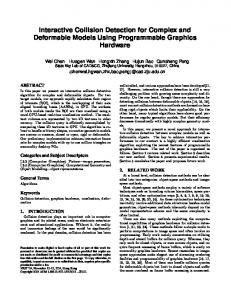
Figure 2: Some scenarios of CCD computation. roots. Equivalently, A (t0 ) and B(t0 ) are separate if and only if F(u,t0 ) = 0 has two distinct real roots u ∈ (0, 1), or F(u,t0 ) > 0, for some u ∈ (0, 1). Otherwise, A (t0 ) and B(t0 ) are either touching externally or overlapping, and F(u,t0 ) ≤ 0, for all 0 < u < 1. Finding all collision intervals. Collision intervals are bounded by 0, 1, or the contact time tˆ, where F(u, tˆ) = 0 has a double root at some uˆ ∈ (0, 1), satisfying F(u, ˆ tˆ) = Fu (u, ˆ tˆ) = 0. It is time-consuming to compute all solutions of F(u,t) = Fu (u,t) = 0 using a straightforward recursive subdivision of F(u,t) over the whole domain (0, 1) × [0, 1]. For better efficiency, we make a good initial guess on collision intervals by applying a sequence of fast separation tests (to static ellipsoids sampled at discrete time intervals 0 = t1 < t2 < · · · < tm = 1). Then we use subdivision either to eliminate intervals which do not contain any solution of F = Fu = 0 or to identify those that contain a unique solution. For the latter intervals, the solution is computed using a novel search scheme, called B´ezier shooting, with quadratic convergence. The sequence of time samples can be divided into three types of segment, giving three cases to consider: (1) Separation of static ellipsoids A (t) and B(t) over a maximal sequence of consecutive samples t = ti ,ti+1 , · · · ,t j . (2) Collision of static ellipsoids A (t) and B(t) over a maximal sequence of consecutive samples t = ti ,ti+1 , · · · ,t j . (3) Transition from separation (t = ti ) to collision (t = ti+1 ), or vice versa. Before treating these cases, we will first explain how B´ezier shooting works. Consider F(u,t) over the domain (0, 1) × [t1 ,t2 ]. Suppose that the two ellipsoids are separate at t1 . B´ezier shooting from t1 to t2 , denoted as BS[t1 → t2 ], has two steps: 1) find uˆ such that Fu (u,t ˆ 1 ) = 0 and F(u,t ˆ 1 ) > 0, by solving a cubic equation; 2) then B´ezier clipping [11] is used from t1 to t2 to either conclude that there is no real root of F(u,t) ˆ in [t1 ,t2 ] (see Fig. 2a) or to compute the smallest root tˆ of F(u,t) ˆ = 0 in [t1 ,t2 ] (see Fig. 2b). In the former case the result of shooting is 5

a miss and the two ellipsoids are separate in [t1 ,t2 ]; in the latter case, shooting scores a hit and tˆ is returned, i.e., tˆ = BS[t1 → t2 ]. Supposing that BS[t1 → t2 ] is a hit, we may use iterative B´ezier shooting by continuing to perform BS[tˆ → t2 ], and so on, to either try to get a miss or converge to a solution of F = Fu = 0. It is proved in Appendix B that the iterative B´ezier shooting has quadratic local convergence. In implementation, if a miss occurs within a fixed number of iterations of B´ezier shooting (we use 4 or 5), we are done and have separation in [t1 ,t2 ]; if there is evidence of convergence after these iterations, we will find the solution (see Fig. 2b); otherwise, the case is undetermined and we use subdivision to get smaller intervals for further processing. If the ellipsoids are separate at t2 , the B´ezier shooting BS[t1 ← t2 ] from t2 to t1 can similarly be defined. Case (1): Consider the interval [ti ,t j ], where the ellipsoids are separate at ti and t j . We first perform BS[ti → t j ] and then BS[ti ← t j ] iteratively. If either is a miss within 4 iterations, we have separation throughout [ti ,t j ]; otherwise, if either does not exhibit convergence (after 4 iterations say), the interval is subdivided. If both iterative shootings converge, denote tk = BS[ti → t j ] and tℓ = BS[ti ← t j ] (see Fig. 2c). If tk = tℓ we have a tangential contact at tk ; otherwise, the interval [tk + δ ,tℓ − δ ], for some small δ < 0, is subdivided at (tk + tℓ )/2 to give two subintervals (see Fig. 2c and 2d), which are in either case (2) or case (3) below. Case (2): Consider the interval [ti ,t j ], where the ellipsoids collide at ti and t j . Having put F(u,t) into bivariate B´ezier form over (0, 1) × [ti ,t j ], we check whether all its control coefficients are negative, which implies collision over the whole interval [ti ,t j ] (see Fig. 2e). If the coefficients are not all negative, we keep subdividing the domain in the t-direction and check the signs of control points. The subdivision will terminate after eliminating all subintervals if there is collision over the whole interval [ti ,t j ]. But if there is separation within [ti ,t j ], recursive subdivision will reduce the problem to instances of the transition case (i.e., case (3)) below. Case (3): Without loss of generality, assume that the ellipsoids are separate at ti and collide at ti+1 (see Fig. 2f). We intend to ensure that there is a unique solution of F = Fu = 0 (i.e. there is no small loop) in [ti ,ti+1 ]. Clearly, there is no loop in [ti ,ti+1 ] if the unit normal vectors ∇F(u,t)/k∇F(u,t)k in [0, 1] × [ti ,ti+1 ] do not cover the whole Gaussian circle. This can be determined efficiently, though conservatively, by checking whether all the 2D control points of ∇F(u,t) are on the same side of a line passing through the origin. If the test is successful, we use iterative B´ezier shooting BS[ti → ti+1 ] to find the unique solution in [ti ,ti+1 ]. If the test fails, we use mid-point subdivision until there is at most one solution of F = Fu = 0 in each subdomain (see Fig. 2f). Finding the first contact time only. Many real-time applications of collision detection require only the first contact time to be computed. Suppose that the two ellipsoids are separate at t = 0. We first sample along the t-direction at t1 ,t2 , . . . until we encounter a collision case at t = tk+1 . Then we perform BS[0 ← tk ]. If the result is a miss (i.e. separation in [0,tk ]), then tk is a good initial value and we use iterative B´ezier shooting BS[tk → tk+1 ] to compute the first contact time. If BS[0 ← tk ] is a hit, we step back to use t = 0 as an initial value and perform iterative shooting BS[0 → tk+1 ] to compute the first contact time. CCD for independent motions. The characteristic equation for two independently moving ellipsoids A (s) and B(t), s,t ∈ [0, 1], is given by F(u, s,t) = det((u − 1)A(s) − uB(t)) = 0. If A (s0 ) and B(t0 ) are separate, then F(u, s0 ,t0 ) = 0 has two distinct roots u ∈ (0, 1); and equivalently, F(u, s0 ,t0 ) > 0, for some u ∈ (0, 1). Otherwise, A (s0 ) and B(t0 ) are either touching externally or overlapping, and F(u, s0 ,t0 ) ≤ 0 for all u ∈ (0, 1). In particular, A (s0 ) and B(t0 ) are touching each other externally if and only if F(u, s0 ,t0 ) = Fu (u, s0 ,t0 ) = 0 for some u ∈ (0, 1). The zero-set of F(u, s,t) = 0 is an algebraic surface in ust-space. Moreover, the common zero-set of F(u, s,t) = Fu (u, s,t) = 0 is an algebraic space curve in ust-space. Let Z denote the curve contained in the cube (0, 1) × 6

[0, 1] × [0, 1]. The projection of Z on to the s-axis covers a union of s-intervals, each of which corresponds to A (s) touching B(t) externally at some t. Thus the s-intervals ‘uncovered’ in this projection correspond to two cases: either (i) A (s) is separate from B(t), for all t, or (ii) A (s) collides with B(t) in interior points, for all t. The end-points of an ‘uncovered’ s-interval are projections of extreme points of the curve Z in the s-direction, which can be classified by the following simultaneous polynomial equations: F(u, s,t) = Fu (u, s,t) = Ft (u, s,t) = 0. The t-intervals ‘uncovered’ in the projection to the t-axis can also be constructed by solving F(u, s,t) = Fu (u, s,t) = Fs (u, s,t) = 0.

5 Experimental Results To demonstrate the effectiveness of our approach, we have implemented a boxing game involving two virtual human characters actively interacting with each other as shown in Fig. 1. Each character is modeled with 24 ellipsoids, representing different body parts such as heads, limbs, etc. The motions of the two boxers are automatically generated by motion capture data, together with a simple control mechanism. All computations are carried out in double precision on a Pentium IV 3GHz CPU. In every time frame, the collision detection algorithm is applied to 576 pairs of ellipsoids, formed by picking one ellipsoid from each of the characters. For each pair of ellipsoids, we first test whether their bounding spheres collide in linear translations. If there is a collision, we compute a plane that separates the two ellipsoids [17] at the beginning of the time frame, and then test whether the two moving ellipsoids are continuously separated by the plane during the whole frame period. We generated 1,000 frames of the boxing animation. As a result, 576,000 pairs of moving ellipsoids were tested. 96.3% of the pairs were filtered out by the sphere test; and 59.0% of the remaining pairs were eliminated using the separating planes. To the remaining 8,837 pairs (1.53%), we applied the algorithm from Section 4 that computes the first contact point in continuous collision detection. Of the 8,837 pairs thus tested, 48.9% were separate and 51.1% were in collision during the time of the frame. In this situation the motions are relatively simple and half of the tests report separations. Thus, for efficiency reason, we directly apply the B´ezier shooting BS[0 → 1] without taking samples until we encounter a collision. Including all the above procedures and the generation of interpolating motions MA (t) and MB (t) for 48 ellipsoids, collision detection for each frame took 3.4 milliseconds, in which 576 pairs of moving ellipsoids were handled. (See the accompanying video and demo.) A continuous rigid motion interpolates the positions and orientations of an ellipsoid between the two ends of each time frame. The center positions are linearly interpolated and the orientations are interpolated by a linear quaternion curve, producing a rotation matrix of rational degree 2. A total of 48 motion matrices were generated in 450 microseconds. The formulation of the bivariate function F(u,t) takes considerable computation; fortunately, we need to compute only 9 (= 576 × 1.53%) such functions on average, which adds very little to the overall computation time. In Fig. 3, two ellipsoids are under dependent motions of degree 4 with relatively large affine deformations. In this example, our system took 3.7 milliseconds to compute all four separation intervals using the algorithm explained in Section 4. Detection of the first contact time only took 0.9 millisecond. Fig. 4 shows the intersection of the swept volumes of two ellipsoids under independent motions and the zeroset surface of F(u, s,t) = 0. In the rightmost two subfigures, the red and blue dots represent the extreme points of ‘uncovered intervals’ in the s- and t-directions, respectively. The four extreme points and the corresponding 7

Figure 3: Two moving ellipsoids under dependent affine deformations, which produce four intersection intervals.

Figure 4: Two moving ellipsoids under independent affine deformations. intersection intervals were computed in 30 milliseconds. But when we processed a similar example with dependent motions, a collision interval was computed in 0.5 millisecond.

6 Conclusions We have presented an exact algorithm for real-time continuous collision detection between two moving ellipsoids under affine motions. It is based on an efficient separation test for two static ellipsoids. A significant speed-up was realized by developing an efficient method called B´ezier shooting, which approximates each regular solution of F = Fu = 0 with quadratic convergence. The special structure of our algebraic condition for separation also allows an efficient test for loop-free domains by checking whether ∇F covers the whole Gaussian circle. We believe that there are many other interesting properties of our algebraic condition, which should lead to more efficient geometric algorithms for dealing with ellipsoids and affine deformations. In future work, we plan to investigate further applications of the computational tools reported in this paper.

References [1] S. Bischoff and L. Kobbelt. Ellipsoid decomposition of 3D-models. In Proc. of 1st Int’l Symp. on 3D Data Processing, Visualization and Transmission (3DPVT 2002), Padova, Italy, June 19–21, pages 480–488, 2002.

8

[2] Y.-K. Choi, W. Wang, and M.-S. Kim. Exact collision detection of two moving ellipsoids under rational motions. In Proc. of the 2003 IEEE Int’l Conference on Robotics and Automation, pages 349–354, 2003. [3] D. H. Eberly. 3D Game Engine Design. Academic Press, 2001. [4] D. H. Eberly. Game Physics. Morgan Kaufmann, 2003. [5] S. Gottschalk, M. Lin, and D. Manocha. OBB-Tree: A hierarchical structure for rapid interference detection. In Proc. of ACM SIGGRAPH’96, pages 171–180, 1996. [6] M. Held, J. Klosowski, and J. Mitchell. Evaluation of collision detection methods for virtual reality flythroughs. In Proc. of the 7th Canadian Conference on Computational Geometry, pages 205–210, 1995. [7] P. Hubbard. Approximating polyhedra with spheres for time-critical collision among spheres. ACM Transactions on Graphics, 15(3):179–210, 1996. [8] D.-E. Hyun, S.-H. Yoon, M.-S. Kim, and B. J¨uttler. Modeling and deformation of arms and legs based on ellipsoidal sweeping. In Proc. of Pacific Graphics 2003, pages 204–212, 2003. [9] M. Ju, J. Liu, S. Shiang, Y. Chien, K. Hwang, and W. Lee. A novel collision detection method based on enclosed ellipsoid. In Proceedings of 2001 IEEE Conference on Robotics and Automation, pages 21–26, 2001. [10] J. Klosowski, M. Held, J. Mitchell, H. Sowizral, and K. Zikan. Efficient collision detection using bounding volume hierarchies of k-dops. IEEE Trans. on Visualization and Computer Graphics, 4(1):21–36, 1998. [11] T. Nishita, T. W. Sederberg, and M. Kakimoto. Ray tracing trimmed rational surface patches. In Proc. of ACM SIGGRAPH’90, pages 337–345, 1990. [12] S. Redon, A. Kheddar, and S. Coquillart. Fast continuous collision detection between rigid bodies. Comput. Graph. Forum, 21(3):279–288, 2002. [13] S. Redon, Y. J. Kim, M. C. Lin, D. Manocha, and J. Templeman. Interactive and continuous collision detection for avatars in virtual environments. In IEEE Virtual Reality Conference 2004 (VR 2004), pages 117–124, 2004. [14] S. Redon, M. C. Lin, D. Manocha, and Y. J. Kim. Fast continuous collision detection for articulated models. ASME J. Comput. Inf. Sci. Eng., 5(2):126–137, 2005. [15] E. Rimon and S. Boyd. Obstacle collision detection using best ellipsoid fit. Journal of Intelligent and Robotic Systems, 18:105–126, 1997. [16] G. van den Bergen. Efficient collision detection of complex deformable models using AABB trees. Journal of Graphics Tools, 2(4):1–13, 1997. [17] W. Wang, Y.-K. Choi, B. Chan, M.-S. Kim, and J. Wang. Efficient collision detection for moving ellipsoids using separating planes. Computing, 72(1-2):235–246, 2004. [18] W. Wang, J. Wang, and M.-S. Kim. An algebraic condition for the separation of two ellipsoids. Comput. Aided Geom. Des., 18(6):531–539, 2001. [19] C. Wu. On the representation and collision detection of robots. Journal of Intelligent and Robotic Systems, 16:151–168, 1996.

9

Appendix A We present an efficient algorithm for computing the five coefficients of the characteristic polynomial f(λ ) of degree 4. Let MAT (MB−1 )T BMB−1 MA = [bi j ]4×4 . Then the characteristic polynomial is given in the following simple form: f(λ ) = det(λ A − MAT (MB−1 )T BMB−1 MA ) λ /a2 − b11 −b12 −b13 −b14 2 −b −b λ /b −b −b24 21 22 23 = 2 λ /c − b33 −b34 −b31 −b32 −b41 −b42 −b43 −λ − b44

.

By expanding this determinant, the five coefficients can be constructed as follows: 1. The 4th-degree term: − a2 b12 c2 2. The 3rd-degree term:

b11 b2 c2

+ ab222c2 + ab233b2 − a2bb442 c2

3. The 2nd-degree term: b33 b44 − b34 b43 b11 b44 − b14 b41 b22 b44 − b24 b42 + + a2 b2 b2 c2 a2 c2 b23 b32 − b22 b33 b13 b31 − b11 b33 b12 b21 − b11 b22 + + + a2 b2 c2

4. The 1st-degree term: −b22 b33 b44 + b22 b34 b43 + b33 b42 b24 b44 b32 b23 − b32 b24 b43 − b42 b23 b34 + a2 a2 −b11 b33 b44 + b11 b34 b43 + b33 b14 b41 b44 b13 b31 − b31 b14 b43 − b41 b13 b34 + + b2 b2 −b11 b22 b44 + b11 b24 b42 + b22 b14 b41 b44 b12 b21 − b21 b14 b42 − b41 b12 b24 + + c2 c2 +b11 b22 b33 − b11 b23 b32 − b22 b13 b31 − b33 b12 b21 + b21 b13 b32 + b31 b12 b23

5. The constant term: b11 b22 b33 b44 − b11 b22 b34 b43 − b11 b33 b24 b42 − b11 b44 b23 b32 −b22 b33 b14 b41 − b22 b44 b13 b31 − b33 b44 b12 b21 +b11 b32 b24 b43 + b11 b23 b34 b42 + b22 b13 b34 b41 +b22 b31 b14 b43 + b33 b12 b24 b41 + b33 b21 b14 b42 + b44 b12 b23 b31 +b44 b21 b13 b32 + b12 b21 b34 b43 + b13 b31 b24 b42 + b14 b41 b23 b32 −b21 b14 b43 b32 − b21 b13 b34 b42 − b31 b12 b24 b43 −b31 b14 b42 b23 − b41 b12 b23 b34 − b41 b13 b32 b24

The following function efficiently computes the five coefficients of the characteristic polynomial using 40 multiplications. Generate-Characteristic-Polynomial /* Variable definition ea,eb,ec is a diagonal member of matrix A ab = ea * eb, ac = ea * ec, bc = eb * ec, abc = ea * eb * ec bij is a member of the matrix MAT (MB−1 )T BMB−1 MA */

10

begin b2233 = b22 * b33; b12s = b12 * b12; b13s = b13 * b13; b14s = b14 * b14; b23s = b23 * b23; b24s = b24 * b24; b34s = b34 * b34; termA = b11 * bc + b22 * ac + b33 * ab; termB = b2233 * ea + b11 * (b33 * eb + b22 * ec); termC = b23s * ea + b13s * eb + b12s * ec; A = −abc; B = termA − b44 * abc; C = termA * b44 − termB + termC −b34s * ab − b14s * bc − b24s * ac; tmp1 = (termB - termC) * b44; tmp2 = b11 * (b2233 + eb * b34s + ec * b24s − b23s); tmp3 = b22 * (ea * b34s + ec * b14s − b13s); tmp4 = b33 * (ea * b24s + eb * b14s − b12s); tmp5 = b34 * (ea * b23 * b24 + eb * b13 * b14) + b12 * ( ec * b14 * b24 − b13 * b23); tmp5 += tmp5; // multiply by 2 D = −tmp1 + tmp2 + tmp3 + tmp4 − tmp5; E = constant; // constant value det[-B] end;

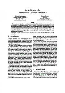
Appendix B t

Fu = 0 F = 0 uˆ

t0

u = kt

t1 u

Figure 5: Quadratic convergence of B´ezier shooting. We will show that iterative B´ezier shooting has quadratic convergence when used to compute a traversal contact time, i.e., a regular solution (u∗ ,t ∗ ) of F(u,t) = Fu (u,t) = 0. Wlog, suppose that (u∗ ,t ∗ ) is located at the origin (0, 0), with F(u,t) = 0 and Fu (u,t) = 0 as shown in Fig. 5. Then, by the regularity assumption and Implicit Function Theorem, the solution of F(u,t) = 0 can be represented locally at (0, 0) by Taylor expansion t = α u2 + o(u2 ), and the solution of Fu (u,t) = 0 by u = kt + o(t). Now consider B´ezier shooting from t0 . The solution of Fu (u,t0 ) = 0 is uˆ = kt0 + o(t0 ). So the first root of F(u,t) ˆ = 0 is t1 = α uˆ2 + o(uˆ2 ) = α [kt0 + o(t0 )]2 + o(t02 ) = α k2t02 + o(t02 ). It follows that t1 /t02 = α k2 + o(1). Hence, B´ezier shooting has quadratic convergence. But if (u∗ ,t ∗ ) is a singular solution representing tangential contact of the two ellipsoids, then the convergence of iterative B´ezier shooting is in general linear. 11