Nowadays, controllers are often implemented as tasks in a real-time kernel and ... The simulated execution time of the code may be modeled as constant, ...
T RUE T IME: Real-time Control System Simulation with MATLAB/Simulink Dan Henriksson, Anton Cervin, Karl-Erik Årzén Department of Automatic Control Lund Institute of Technology Box 118, SE-221 00 Lund, Sweden {dan,anton,karlerik}@control.lth.se Abstract: Traditional control design using MATLAB/Simulink, often disregards the temporal effects arising from the actual implementation of the controllers. Nowadays, controllers are often implemented as tasks in a real-time kernel and communicate with other nodes over a network. Consequently, the constraints of the target system, e.g., limited CPU speed and network bandwidth, must be taken into account at design time. For this purpose we have developed T RUE T IME, a toolbox for simulation of distributed real-time control systems. T RUE T IME makes it possible to simulate the timely behavior of real-time kernels executing controller tasks. T RUE T IME also makes it possible to simulate simple models of network protocols and their influence on networked control loops. T RUE T IME consists of a kernel block and a network block, both variable-step S-functions written in C++. T RUE T IME also provides a collection of MATLAB functions used to, e.g., do A/D and D/A conversion, send and receive network messages, set up timers, and change task attributes. The T RUE T IME blocks are connected with ordinary continuous Simulink blocks to form a real-time control system. The T RUE T IME kernel block simulates a computer with an event-driven real-time kernel, A/D and D/A converters, a network interface, and external interrupt channels. The kernel executes user-defined tasks and interrupt handlers, representing, e.g., I/O tasks, control algorithms, and communication tasks. Execution is defined by user-written code functions (C++ functions or m-files) or graphically using ordinary discrete Simulink blocks. The simulated execution time of the code may be modeled as constant, random or even data-dependent. Furthermore, the real-time scheduling policy of the kernel is arbitrary and decided by the user. The T RUE T IME network block is event driven and distributes messages between computer nodes according to a chosen network model. Currently five of the most common medium access control protocols are supported (CSMA/CD (Ethernet), CSMA/CA (CAN), token-ring, FDMA, and TDMA). It is also possible to specify network parameters such as transmission rate, pre- and post-processing delays, frame overhead, and loss probability. T RUE T IME is currently used as an experimental platform for research on flexible approaches to real-time implementation and scheduling of controller tasks. One example is feedback scheduling where feedback is used in the real-time system to dynamically distribute resources according to the current situation in the system.
1. Introduction Control systems are becoming increasingly complex from the perspectives of both control and computer science. Today, even seemingly simple embedded control systems often contain a multitasking real-time kernel and support networking. At the same time, the market demands that the cost of the system be kept at a minimum. For optimal use of computing resources, the control algorithm and the control software designs need to be considered at the same time. For this reason, new, computer-based tools for real-time and control co-design are needed. Many computer-controlled systems are distributed systems consisting of computer nodes and a communication network connecting the various systems. It is not uncommon for the sensor, the actuator, and the control calculations to reside on different nodes, as in vehicle systems, for example. This gives rise to networked control loops (see [1]). Within the individual nodes, the controllers are often implemented as one or several tasks on a microprocessor with a real-
time operating system. Often the microprocessor also contains tasks for other functions (e.g., communication and user interfaces). The operating system typically uses multiprogramming to multiplex the execution of the various tasks. The CPU time and the communication bandwidth can hence be viewed as shared resources for which the tasks compete. Digital control theory normally assumes equidistant sampling intervals and a negligible or constant control delay from sampling to actuation. However, this can seldom be achieved in practice. Within a node, tasks interfere with each other through preemption and blocking when waiting for common resources. The execution times of the tasks themselves may be data-dependent or may vary due to hardware features such as caches. On the distributed level, the communication gives rise to delays that can be more or less deterministic depending on the communication protocol. Another source of temporal nondeterminism is the increasing use of commercial off-the-shelf (COTS) hardware and software components in real-time control (e.g., general-
purpose operating systems such as Windows and Linux and general-purpose network protocols such as Ethernet). These components are designed to optimize average-case rather than worst-case performance. The temporal nondeterminism can be reduced by the proper choice of implementation techniques and platforms. For example, time-driven static scheduling improves the determinism, but at the same time it reduces the flexibility and limits the possibilities for dynamic modifications. Other techniques of similar nature are time-driven architectures such as TTA [5] and synchronous programming languages such as Esterel, Lustre, and Signal [4]. With these techniques, however, a certain level of temporal nondeterminism is still unavoidable. The delay and jitter introduced by the computer system can lead to significant performance degradation. To achieve good performance in systems with limited computer resources, the constraints of the implementation platform must be taken into account at design time. To facilitate this, software tools are needed to analyze and simulate how the timing affects the control performance. This paper describes T RUE T IME1 , which is MATLAB toolbox facilitating simulation of the temporal behavior of a multitasking real-time kernel executing controller tasks. The tasks are controlling processes that are modeled as ordinary Simulink blocks. T RUE T IME also makes it possible to simulate simple models of communication networks and their influence on networked control loops. Different scheduling policies may be used (e.g., priority-based preemptive scheduling and earliest-deadline-first (EDF) scheduling, see, e.g., [6]. T RUE T IME is currently used as an experimental platform for research on dynamic real-time control systems. For instance, it is possible to study compensation schemes that adjust the control algorithm based on measurements of actual timing variations (i.e., to treat the temporal uncertainty as a disturbance and manage it with feedforward or gain scheduling). It is also easy to experiment with more flexible approaches to real-time scheduling of controllers, such as feedback scheduling [3]. There the available CPU or network resources are dynamically distributed according the current situation (CPU load, the performance of the different loops, etc.) in the system.
2. Simulation Environment T RUE T IME consists of a block library with a computer kernel block and a network block, as shown in Fig. 1. The blocks are variable-step, discrete, MATLAB S-functions written in C++. The computer block executes user-defined tasks and interrupt handlers representing, e.g., I/O tasks, control algorithms, and network interfaces. The scheduling policy of the individual computer blocks is arbitrary and decided by the user. The network block distributes messages 1 Available at
http://www.control.lth.se/˜dan/truetime
Figure 1 The T RUE T IME block library. The Schedule and Monitor outputs display the allocation of common resources (CPU, monitors, network) during the simulation.
between computer nodes according to a chosen network model. Both blocks are event-driven, with the execution determined both by internal and external events. Internal events are timely and correspond to events such as “a timer has expired,” “a task has finished its execution,” or “a message has completed its transmission.” External events correspond to external interrupts, such as “a message arrived on the network” or “the crank angle passed zero degrees.” The block inputs are assumed to be discrete-time signals, except the signals connected to the A/D converters of the computer block, which may be continuous-time signals. All outputs are discrete-time signals. The Schedule and Monitors outputs display the allocation of common resources (CPU, monitors, network) during the simulation. The level of simulation detail is chosen by the user—it is often neither necessary nor desirable to simulate code execution on instruction level or network transmissions on bit level. T RUE T IME allows the execution time of tasks and the transmission times of messages to be modeled as constant, random, or data-dependent. Furthermore, T RUE T IME allows simulation of context switching and task synchronization using events or monitors. 2.1 The Computer Block The computer block S-function simulates a computer with a simple but flexible real-time kernel, A/D and D/A converters, a network interface, and external interrupt channels. Internally, the kernel maintains several data structures that are commonly found in a real-time kernel: a ready queue, a time queue, and records for tasks, interrupt handlers, monitors and timers that have been created for the simulation. The execution of tasks and interrupt handlers is defined by user-written code functions. These functions can be written either in C++ (for speed) or as MATLAB m-files (for ease of use). Control algorithms may also be defined graphically using ordinary discrete Simulink block diagrams.
Tasks The task is the main construct in the T RUE T IME simulation environment. Tasks are used to simulate both periodic activities, such as controller and I/O tasks, and aperiodic activities, such as communication tasks and event-driven controllers. An arbitrary number of tasks can be created to run in the T RUE T IME kernel. Each task is defined by a set of attributes and a code function. The attributes include a name, a release time, a worst-case execution time, an execution time budget, relative and absolute deadlines, a priority (if fixedpriority scheduling is used), and a period (if the task is periodic). Some of the attributes, such as the release time and the absolute deadline, are constantly updated by the kernel during simulation. Other attributes, such as period and priority, are normally kept constant but can be changed by calls to kernel primitives when the task is executing. In accordance with [2], it is furthermore possible to attach two overrun handlers to each task: a deadline overrun handler (triggered if the task misses its deadline) and an execution time overrun handler (triggered if the task executes longer than its worst-case execution time). Interrupts and Interrupt Handlers Interrupts may be generated in two ways: externally or internally. An external interrupt is associated with one of the external interrupt channels of the computer block. The interrupt is triggered when the signal of the corresponding channel changes value. This type of interrupt may be used to simulate engine controllers that are sampled against the rotation of the motor or distributed controllers that execute when measurements arrive on the network. Internal interrupts are associated with timers. Both periodic timers and one-shot timers can be created. The corresponding interrupt is triggered when the timer expires. Timers are also used internally by the kernel to implement the overrun handlers described in the previous section. When an external or internal interrupt occurs, a user-defined interrupt handler is scheduled to serve the interrupt. An interrupt handler works much the same way as a task, but is scheduled on a higher priority level. Interrupt handlers will normally perform small, less time-consuming tasks, such as generating an event or triggering the execution of a task. An interrupt handler is defined by a name, a priority, and a code function. External interrupts also have a latency during which they are insensitive to new invocations. Priorities and Scheduling Simulated execution occurs at three distinct priority levels: the interrupt level (highest priority), the kernel level, and the task level (lowest priority). The execution may be preemptive or non-preemptive; this can be specified individually for each task and interrupt handler. At the interrupt level, interrupt handlers are scheduled according to fixed priorities. At the task level, dynamicpriority scheduling may be used. At each scheduling point,
Execution of user code
1
2
3
Simulated execution time Figure 2 The execution of the code associated with tasks and interrupt handlers is modeled by a number of code segments with different execution times. Execution of user code occurs at the beginning of each code segment.
the priority of a task is given by a user-defined priority function, which is a function of the task attributes. This makes it easy to simulate different scheduling policies. For instance, a priority function that returns a priority number implies fixed-priority scheduling, whereas a priority function that returns a deadline implies deadline-driven scheduling. Predefined priority functions exist for most of the commonly used scheduling schemes. Code The code associated with tasks and interrupt handlers is scheduled and executed by the kernel as the simulation progresses. The code is normally divided into several segments, as shown in Fig. 2. The code can interact with other tasks and with the environment at the beginning of each code segment. This execution model makes it possible to model input-output delays, blocking when accessing shared resources, etc. The simulated execution time of each segment is returned by the code function, and can be modeled as constant, random, or even data-dependent. The kernel keeps track of the current segment and calls the code functions with the proper argument during the simulation. Execution resumes in the next segment when the task has been running for the time associated with the previous segment. This means that preemption from higher-priority activities and interrupts may cause the actual delay between the segments to be longer than the execution time. Fig. 3 shows an example of a code function corresponding to the time line in Fig. 2. The function implements a simple controller. In the first segment, the plant is sampled and the control signal is computed. In the second segment, the control signal is actuated and the controller states are updated. The third segment indicates the end of execution by returning a negative execution time. The functions calculateOutput and updateState are assumed to represent the implementation of an arbitrary controller. The data structure data represents the local memory of the task and is used to store the control signal and measured variable between calls to the different segments. A/D and D/A conversion is performed using the kernel primitives ttAnalogIn and ttAnalogOut.
function [exectime, data] = myController(seg, data) switch seg, case 1, data.y = ttAnalogIn(1); data.u = calculateOutput(data.y); exectime = 0.002; case 2, ttAnalogOut(1, data.u); updateState(data.y); exectime = 0.003; case 3, exectime = -1; % finished end Figure 3
Example of a simple code function.
Table 1 Examples of kernel primitives (pseudo syntax) that can be called from code functions associated with tasks and interrupt handlers. ttAnalogIn(ch)
Get the value of an input channel
ttAnalogOut(ch, val) ttSendMsg(rec,data,len)
Set the value of an output channel
ttGetMsg()
Get message from network input queue
ttSleepUntil(time)
Wait until a specific time
ttCurrentTime()
Current time in simulation
ttCreateTimer(time,ih) ttEnterMonitor(mon)
Trigger interrupt handler at a specific time
ttWait(ev)
Await an event
ttNotifyAll(ev)
Activate all tasks waiting for an event
ttSetPriority(val)
Change the priority of a task
ttSetPeriod(val)
Change the period of a task
Send message over network
Enter a monitor
Besides A/D and D/A conversion, many other kernel primitives exist that can be called from the code functions. These include functions to send and receive messages over the network, create and remove timers, perform monitor operations, and change task attributes. Some of the kernel primitives are listed in Table 1. As an alternative to textual implementation of the controller algorithms, T RUE T IME also allows for graphical representation of the controllers. Controllers represented using ordinary discrete Simulink blocks may be called from within the code functions to calculate control actions. Synchronization Synchronization between tasks is supported by monitors and events. Monitors are used to guarantee mutual exclusion when accessing common data. Events can be associated with monitors to represent condition variables. Events may also be free (i.e., not associated with a monitor). This feature can be used to obtain synchronization between tasks where no conditions on shared data are involved. The example in Fig. 4 shows the use of a free event input_event to simulate an event-driven controller task. The corresponding ttNotifyAll-call of the event is typically performed in an interrupt handler associated with an external interrupt port.
function [exectime, data] = eventController(seg, data) switch (segment), case 1, ttWait(’input_event’); exectime = 0.0; case 2, data.y = ttAnalogIn(1); data.u = calculateOutput(data.y); exectime = 0.002; case 3, ttAnalogOut(1, data.u); updateState(data.y); exectime = 0.003; case 3, ttSetNextSegment(1); % loop end Figure 4 Example of a code function implementing an eventbased controller.
Output Graphs Depending on the simulation, several different output graphs are generated by the T RUE T IME blocks. Each computer block will produce two graphs, a computer schedule and a monitor graph, and the network block will produce a network schedule. The computer schedule will display the execution trace of each task and interrupt handler during the course of the simulation. If context switching is simulated, the graph will also display the execution of the kernel. For an example of such an execution trace, see Fig. 9. If the signal is high it means that the task is running. A medium signal indicates that the task is ready but not running (preempted), whereas a low signal means that the task is idle. In an analogous way, the network schedule shows the transmission of messages over the network, with the states representing sending (high), waiting (medium), and idle (low). The monitor graph shows which tasks are holding and waiting on the different monitors during the simulation. Generation of these execution traces is optional and can be specified individually for each task, interrupt handler, and monitor. 2.2 The Network Block The network model is similar to the real-time kernel model, albeit simpler. The network block is event-driven and executes when messages enter or leave the network. A message contains information about the sending and the receiving computer node, arbitrary user data (typically measurement signals or control signals), the length of the message, and optional real-time attributes such as a priority or a deadline. In the network block, it is possible to specify the transmission rate, the medium access control protocol (CSMA/CD, CSMA/CA, round robin, FDMA, or TDMA), and a number of other parameters, see Fig. 5. A long message can be split into frames that are transmitted in sequence, each with an additional overhead. When the simulated transmission of a message has completed, it is put in a buffer at the receiving computer node, which is notified by a hardware interrupt.
%% Code function for the actuator task function [exectime, data] = actcode(seg, data) switch seg, case 1, ttWait(’packet’); exectime = 0.0; case 2, data.u = ttGetMsg; exectime = 0.0005; case 3, ttAnalogOut(1, data.u); ttSetNextSegment(1); % wait for new msg exectime = 0.0; end %% Code function for the network interrupt handler function [exectime, data] = msgRcvHandler(seg, data) ttNotifyAll(’packet’); exectime = -1; %% Initialization function %% creating the task, interrupt handler and event function actuator_init nbrOfInputs = 0; nbrOfOutputs = 1; ttInitKernel(nbrOfInputs, nbrOfOutputs, ’prioFP’);
Figure 5
The dialogue of the T RUE T IME Network block.
3. Example: A Networked Control System Using T RUE T IME, general simulation of a distributed control system is possible wherein the effects of scheduling in the CPUs and simultaneous transmission of messages over the network can be studied in detail. T RUE T IME allows experimentation with different scheduling policies of CPU and network and different compensation schemes to cope with induced delays. The T RUE T IME simulation model of the system contains four computer nodes connected by one network block. The time-driven sensor node contains a periodic task, which at each invocation samples the process and transmits the sample package to the controller node. The controller node contains an event-driven task that is triggered each time a sample arrives over the network from the sensor node. Upon receiving a sample, the controller computes a control signal, which is then sent to the event-driven actuator node, where it is actuated. The model also contains an interference node with a periodic task generating random interfering traffic over the network. 3.1 Initialization of the Actuator Node As a complete initialization example, Fig. 6 shows the code needed to initialize the actuator node in this particular example. The computer block contains one task and one interrupt handler, and their execution is defined by the code functions actcode and msgRcvHandler, respectively. The task and interrupt handler are created in the actuator_init function together with an event (packet) used to trigger the execution of the task. The node is “connected” to the
priority = 5; deadline = 0.010; release = 0.0; ttCreateTask(’act_task’, deadline, priority, ’actcode’); ttCreateJob(’act_task’, release); ttCreateInterruptHandler(’msgRcv’, 1, ’msgRcvHandler’); ttInitNetwork(2, ’msgRcv’); % I am node 2 ttCreateEvent(’packet’);
Figure 6 Complete initialization of the actuator node in the networked control system simulation.
network in the function ttInitNetwork by supplying a node identification number and the interrupt handler to be executed when a message arrives to the node. In the ttInitKernel function the kernel is initialized by specifying the number of A/D and D/A channels and the scheduling policy. The built-in priority function prioFP specifies fixed-priority scheduling. Other predefined scheduling policies include rate monotonic (prioRM), earliest deadline first (prioEDF), and deadline monotonic (prioDM) scheduling. 3.2 Experiments In the following simulations, we will assume a CAN-type network where transmission of simultaneous messages is decided based on package priorities. The controller node contains a PD-controller task with a 10-ms sampling interval. The same sampling interval is used in the sensor node. In a first simulation, all execution times and transmission times are set equal to zero. The control performance resulting from this ideal situation is shown in Fig. 7. Next we consider a more realistic simulation where execution times in the nodes and transmission times over the net-
Reference Signal (dashed) and Measurement Signal (full)
Reference Signal (dashed) and Measurement Signal (full)
1.5
1.5
1
1
0.5
0.5
0
0
−0.5
0
0.1
0.2
0.3 0.4 Control Signal
0.5
0.6
−0.5
2
2
1
1
0
0
−1
−1
−2
0
0.1
0.2
0.3 Time [ms]
0.4
0.5
0.6
Figure 7 Control performance without time delay.
work are taken into account. The execution time of the controller is 0.5 ms and the ideal transmission time from one node to another is 1.5 ms. The ideal round-trip delay is thus 3.5 ms. The packages generated by the interference node have high priority and occupy 50% of the network bandwidth. We further assume that an interfering, high-priority task with a 7-ms period and a 3-ms execution time is executing in the controller node. Colliding transmissions and preemption in the controller node will thus cause the roundtrip delay to be even longer on average and time-varying. The resulting degraded control performance can be seen in the simulated step response in Fig. 8. The execution of the tasks in the controller node and the transmission of messages over the network can be studied in detail (see Fig. 9). Finally, a simple compensation is introduced to cope with the delays. The packages sent from the sensor node are now time-stamped, which makes it possible for the controller to determine the actual delay from sensor to controller. The total delay is estimated by adding the expected value of the delay from controller to actuator. The control signal is then calculated based on linear interpolation among a set of controller parameters pre-calculated for different delays. Using this compensation, better control performance is obtained, as seen in Fig. 10.
−2
0
0.1
0.2
0
0.1
0.2
0.3 0.4 Control Signal
0.3 Time [ms]
0.4
0.5
0.6
0.5
0.6
Figure 8 Control performance with interfering network messages and interfering task in the controller node. Network Schedule
Interf. Node Controller Node Sensor Node 0
0.02
0.04
0.06
0.08
0.1
0.08
0.1
Computer Schedule
Interf. Thread
Controller Thread 0
0.02
0.04
0.06 Time [s]
Figure 9 Close-up of schedules showing the allocation of common resources: network (top) and controller node (bottom). A high signal means sending or executing, a medium signal means waiting, and a low signal means idle. Reference Signal (dashed) and Measurement Signal (full) 1.5
References
1
[1] Special Section on Networks and Control, IEEE Control Systems Magazine, vol. 21. February 2001.
0.5
[2] G. Bollella, B. Brosgol, P. Dibble, S. Furr, J. Gosling, D. Hardin, and M. Turnbull. The Real-Time Specification for Java. Addison-Wesley, 2000.
−0.5
[3] A. Cervin, J. Eker, B. Bernhardsson, and K.-E. Årzén. “Feedbackfeedforward scheduling of control tasks.” Real-Time Systems, 23, pp. 25–53, 2002. [4] N. Halbwachs. Synchronuous Programming of Reactive Systems. Kluwer, Boston, MA, 1993. [5] H. Kopetz. Real-Time Systems: Design Principles for Distributed Embedded Applications. Kluwer, Boston, MA, 1997. [6] J. W. S. Liu. Real-Time Systems. Prentice-Hall, 2000.
0 0
0.1
0.2
0
0.1
0.2
0.3 0.4 Control Signal
0.5
0.6
0.5
0.6
2 1 0 −1 −2
0.3 Time [ms]
0.4
Figure 10 Control performance with delay-compensation.