REAL-TIME IMAGE SUPER RESOLUTION USING AN FPGA Oliver Bowen, Christos-Savvas Bouganis Department of Electrical and Electronic Engineering Imperial College London London, UK email:
[email protected],
[email protected] ABSTRACT Image super resolution is the process of combining a set of overlapping low-resolution images to produce a single highresolution image. In this paper, a novel real-time superresolution system is presented which is based on a weighted mean super-resolution algorithm combined with the existing fast and robust multi-frame super-resolution algorithm. The resource requirements of the proposed architecture scale linearly with the targeted image quality, making it ideally suited for a variety of real-time applications such as HDTV. Simulation results demonstrate a speed-up of three orders of magnitude over optimized software implementations with negligible loss to image quality.
Fig. 1. SR image reconstruction from a series of LR frames. FPGA based SR system based on the iterative back projection method is presented. The architecture presented in [5] requires memory access to all low-resolution (LR) frames used in the high-resolution (HR) estimate, and results are computed only after multiple passes through the hardware. This work proposes a modification to an existing SR algorithm and an architecture mapping of this algorithm into hardware. Contrary to the previous work, the presented architecture requires memory access to only two LR frames, and deblurring and image sharpening are performed. The resulting system is capable of real-time performance on large image sizes, and high frame rates, such as those encountered in HDTV. For this system, an FPGA device is targeted, since it can be reconfigured in run-time to match the system requirements for image quality. In this work, we assume the motion parameters are given and focus only on the reconstruction problem.
1. INTRODUCTION Applying image processing techniques to improve the quality of digital images has been an active area of study for many decades. There is however a limit to how much one can improve image quality using single-frame image processing techniques. Image super-resolution (SR) aims to overcome this limit by combining the information present in a series of non-identical overlapping frames. Fig. 1 provides an example of SR. Real-time image super-resolution is the ability to perform SR on a set of input frames at a rate suitable for high speed applications, such as consumer video up-conversion, medical imaging, surveillance, and quality control. The majority of the work published on SR to date focuses on the mathematical algorithms behind SR and the ability to overcome inherent obstacles such as noise, non-uniform blur, and motion estimation errors. Some of the literature addresses the computational efficiency of SR techniques [1, 2, 3], but as is shown in this work, the scalability of these solutions in real-time applications is poor. A hardware based SR system is presented in [4] which makes use of existing motion estimations from a decoding block and aims to minimize the memory cost. Their approach makes use of very long instruction words (VLIW) and ARM processors, and no deblurring or image sharpening is performed. In [5] an
978-1-4244-1961-6/08/$25.00 ©2008 IEEE.
2. SUPER RESOLUTION BACKGROUND Image SR relies on the ability to recover high-frequency content from aliased data present in a series of LR frames. This is possible if spatial or temporal sub-pixel motion exists between the LR frames so that each frame contains different sets of pixels of the same scene. If the motion between the frames is known or can be estimated, the LR pixels can be mapped onto appropriate positions on a HR grid. Various approaches to SR have been developed in the literature [1]. These can be broadly divided into frequency and
89
The solution to this problem is shown in [6] to be the maximum likelihood estimator. Direct solutions to this estimator require computing the inverse of very large matricies making it unsuitable for use on large images. Instead iterative solutions such as the steepest descent (SD) are used to ˆ [2]. solve for X Fig. 2. Image acquisition system model. 2.3. Computationally Efficient Super Resolution
spatial domain approaches. In this work, computationally efficient spatial domain solutions are considered, as these demonstrated the most promise for hardware acceleration.
In [2] various assumptions are made regarding the nature of the acquired LR images, and it is shown that the solution to which the SD method converges, can be simplified to a non-iterative equation. One of these assumptions is that the blur operations are the same for each frame, which means ˆ and then ˆ of X, one can first solve for the blurred version Z remove the blur at a later stage. The algorithm given in [2] ˆ is to find Z
2.1. Modelling the Super Resolution Problem An ideal solution to the SR problem reconstructs the same HR scene from which a series of LR images was originally down-sampled from. To achieve this, the LR frames must undergo the inverse of the degradation caused by the imaging system. Since the model parameters must be inferred from the LR images, SR is an ill-posed inverse problem [1]. A general model representing the various stages of degradation present in an imaging system can be seen in Fig. 2. In this model, all captured images undergo the same atmospheric and motion blur. The warp operation represents translations or rotations of the HR scene, which results in the acquisition of unique images. These images are subject to additional blur due to the camera lens and are downsampled by the imaging device. The various stages of this model can be represented mathematically by matrix operations. Equation (1) describes the aquisition of a series of N LR frames. Y k = Dk Hkcam Fk Hkatm X + V k
, k = 1, 2, ..., N
ˆ = R−1 P Z where R =
k=1
(3)
k=1
In [3], a fast and robust iterative SR algorithm is proposed. The algorithm makes use of L1-norm minimization and robust regularization techniques to deal with motion estimation errors and inaccurate blur models. The regularization function is based on total variation and a type of bilateral filtering, which can be implemented efficiently as a series of shift-and-add operations. The result is a robust SR algorithm capable of reducing noise and sharpening edges. The solution to the modified minimization problem is given in (4). The L1-norm is shown in [3] to be equivalent to a pixelwise median estimator, and is used to obtain X0 , the starting
[Y k − Dk Hk Fk X]T [Y k − Dk Hk Fk X]}
k=1
FkT DT Y k
2.4. Efficient and Robust Super Resolution
One approach to solve the SR problem is to find the image ˆ which when fed into the model described above, proX, duces a set of LR images that minimizes the mean squared difference between this set and the original set Y k . Equation (2) describes this minimization without taking the noise into account, and by combining the atmospheric and camera blur matricies, which commute under certain conditions [3].
X
N !
This algorithm performs very well when the motion estimates are accurate and can be rounded to integer shifts in the HR grid. In the presence of outliers due to noise or motion estimation errors, our simulations showed that the quality of the SR results degrades rapidly.
(1)
2.2. Super-Resolution as a Minimization Problem
N !
FkT DT DFk , P =
This algorithm can be implemented very efficiently if all the warp operations Fk are purely translational. The result of each pixel in Zˆ is a mean of all the LR pixels which map to its location. Any missing pixels in Zˆ can be interpolated from neighbouring pixels. Further processing is required to deblur the resulting high resolution image.
In (1) Y and X are column vectors representing the k LR and HR images. D, H, and V are matricies modelling the decimation, blurring and additive noise of the system.
ˆ = argmin{ X
N !
(2)
90
point for the algorithm.
Equation (3) has been modified to include the weight matrix Wk , which has the same dimensions as the LR image matrix Yk . The modified equation is given in (5).
ˆ − β{H T AT sign(AH X ˆ − AZ)+ ˆ =X X n+1 n n
λ
P P ! !
l=−P m=0
"
#$
l+m≥0
ˆ − Sym Sxl )} α|m|+|l| [I − Sy−m Sx−l ]sign(X n
%
ˆ = R−1 P Z where R =
(4)
N !
FkT DT Wk
and P =
k=1
In (4), A is a diagonal matrix whose elements correspond to the square root of the number of LR pixels that contribute to each pixel in Z. This ensures that missing pixels in Z do not effect the iterative estimate of X, while those derived from many LR pixels have the most effect [3]. Sy−m and Sx−l represent shifts of m and l pixels in the y and x directions. β represents the step size, α, 0 < α < 1, applies a spatially decaying weight, and γ is a weight to the regularization term. Although the algorithm is iterative in nature, each iterative stage can be implemented efficiently because only pixel by pixel operations are performed.
N !
k=1
FkT DT (Yk · Wk ) (5)
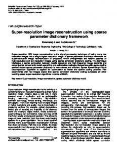
In (5), where · represents an element by element multiplication, R stores the cumulative sum of the weights of each LR pixel mapping to a particular SR coordinate, while P stores the cumulative sum of the pixel values multiplied by their weights. 3.2. Combining the Algorithms Our weighted mean algorithm is able to eliminate outliers when multiple LR pixels map to the same HR coordinate. It does not however perform any deblurring or denoising. The iterative algorithm described in section 2.4 performs deblurring and regularization, which helps to further reduce the visibility of outliers and noise. In this work, we propose using our weighted mean algorithm as a starting point for the iterative algorithm instead of the pixel-wise median proposed in [3]. Results confirm that this approach yields superior image quality after fewer iterations. Fig. 3 compares the SR results of the weighted mean algorithm (Section 3.1), the iterative algorithm (Section 2.4), and the proposed combined algorithm, when using a set of 25 LR frames after 25 iterations. The frames were obtained by downsampling a randomly shifted and blurred HR image, and adding zero-mean gaussian noise, resulting in images with a PSNR of 78 dB. Salt-and-pepper noise affecting 2% of pixels was also added. Four of the twenty-five frames contained random motion estimation errors. In Fig. 4, the robustness of the iterative and combined algorithms is compared using the same test image. The mean squared error of the image results when compared to the original HR image is plotted against the number of motion estimation errors present in the set of 25 LR frames. The combined system demonstrates superior robustness for the same number of iterations when compared to the iterative algorithm.
3. THE PROPOSED ALGORITHM In this section, a modified version of the algorithm described in section 2.3, based on a weighted mean approach, is proposed for the initial estimate. This algorithm calculates a blurred version of the HR image. In order to deblur this estimated HR image, the algorithm is combined with the iterative approach described in section 2.4, resulting in a realtime algorithm suitable for implementation on an FPGA. 3.1. The Weighted Mean Approach The algorithm described in [2] is computationally efficient, but lacks robustness in the presence of outliers. In order to reduce the impact of the outliers caused by motion estimation errors, rotations, or parallax, we propose to weight the pixels according to the accuracy of their frame’s motion estimate. Pixels in the regions that match the reference frame very closely were given a high weight, while those that matched very poorly were given a low weight. When two or more LR pixels map to the same location on the HR grid, the weighted mean of these pixels can be used to calculate the new SR pixel. To calculate the pixel weights, the frame was shifted by the inverse of its motion estimate, and a 3-by-3 window around each pixel was compared to the same region in the reference frame. The sum of the absolute difference of the 9 pixels was calculated and raised to a power p. The purpose of p is to ensure that the pixels from frames with accurate motion estimates significantly out-weigh pixels from frames with poor motion estimates. In this work, we determined that a value of p = 4 was suitable.
3.3. Modifications for Real Time The algorithms covered so far combine a set of LR frames into a single HR frame. In real-time applications, a continuous sequence of HR images is generally required. To accomplish this, a moving window of n LR frames is used to calculate each HR frame. When a change of scene occurs, the previous LR frames are discarded, and the SR results
91
Mean squared error compared to HR original
(a)
(b)
1400 1300 1200
Iterative Algorithm (10 iter.) Combined Algorithm (10 iter.) Iterative Algorithm (20 iter.) Combined Algorithm (20 iter.)
1100 1000 900 800 700 600 500 0 2 4 6 8 10 12 14 Number of LR frames containing motion estimation errors
Fig. 4. Comparing the robustness of SR algorithms.
(c)
overview of the architecture of the system. The window of LR frames is stored in RAM 1, from which the motion estimates as well as the old and new pixel and weight pairs are read. The LR pixels are mapped to the appropriate HR coordinate and merged with information from the previous result which is stored in either RAM 2 or RAM 3. Using all of this information, (6) is implemented on a per pixel basis, and the result is passed directly to the interpolation block. In addition to this, the result is stored in either RAM 2 or RAM 3 for future use. The interpolation block implements a pipelined convolution to fill in missing pixels. The output of this block is used as the starting point for the iterative stages which refine the SR result and output this to RAM 4. The entire design is pipelined and is able to calculate one new SR pixel per clock cycle. Architectural details of the sub blocks are presented in the following sections.
(d)
Fig. 3. Comparison of algorithms. (a) 1 of 25 LR frames. (b) Result using weighted mean algorithm. (c) Result using iterative algorithm. (d) Result using combined algorithm. rely on interpolation until additional LR frames of the new scene can be used. The combined algorithm was modified for such a realtime system. This involved two primary changes. First, the motion of each frame was calculated relative to the position of the previous frame. Second, instead of reconstructing each SR frame directly from n LR frames, the previous SR result was used as a starting point. This allowed the next SR frame to be calculated by simply adding information from the newest LR frame and subtracting information from the nth LR frame, as is shown in (6). # PSR
PSR WSR + P1 W1 − Pn Wn = WSR + W1 − Wn # WSR = WSR + W1 − Wn
4.1. The Weighted Mean System The weighted mean system is made up of three blocks which perform pixel mapping and RAM access, arithmetic operations, and interpolation. 4.1.1. Pixel Mapping and RAM Access At the start of each frame the motion estimate is read from the RAM and used to determine the mapping of the LR pixels. An LR pixel is said to map to a particular SR coordinate if, after up-sampling and shifting, its position on the HR grid corresponds to that SR coordinate. The previous SR result is shifted by the inverse of this motion estimate, so that the new SR result will always be centered over the same position in the scene as the current LR frame.
(6)
# # and WSR are the new SR pixel intensity and In (6), PSR cumulative weight. PSR and WSR , are the previous frame’s SR pixel intensity and weight, P1 ,W1 ,Pn , and Wn are the the new and old LR pixel intensities and weights.
4.1.2. Merge Pixel Arithmetic
4. FPGA IMPLEMENTATION
The second stage of the merge-pixel block implements (6) to calculate the new SR pixel value and weight. The operations are pipelined ensuring that no more than one addition or multiplication takes place each cycle. The division was
The combined algorithm described in the previous section was mapped onto hardware using fixed-point precision and a highly pipelined architecture. Fig. 5 shows a high-level
92
Fig. 5. System Architecture. implemented as a reciprocal multiplication using a look-up table with 28 entries, since the pixel intensities are stored as 8 bit values. 4.2. The Interpolation Block A pipelined form of two dimensional convolution is used to interpolate the missing pixels. This involves storing the k previous image rows in FIFOs, and the k previous pixels from each row in registers, so that a k × k window of pixels is available each cycle. A modified form of nearestneighbor interpolation was implemented in which only pixels with non-zero weights are used to interpolate the missing pixels. The number of pixels in the convolution window that contain non-zero weights is used to select one of many predefined coefficients for use in the filter. The FIFOs were implemented using embedded RAMs, and the access pattern to these is deterministic given the frame translational parameters.
Fig. 6. Architecture of a single iterative stage. bits required. Pixels were represented using 8 bits, and 2 bits were added for the fractional results of the iterative stages. The architecture for a single iterative stage is shown in Fig. 6. Incoming pixels are stored in FIFO line buffers so that a 5 × 5 window of pixel data is available. This data is then fed into two parallel datapaths. The first performs the blur operation H, the multiplication by A, the sign operation, and the sharpening operation H −1 . Both H and H −1 operations make use of pipelined convolution. The second path implements the shift-and-add operations. The results from each path are combined and passed to the next iterative stage.
4.3. Implementation of the Iterative Stages The formula described in (4) was implemented in hardware by observing that each iteration could be treated as a separate stage in a long pipeline. Each iterative stage requires, as inputs, the pixel value from the previous iteration Xn , the original pixel value Z, and A. Z and A are buffered within each stage and passed unchanged to the subsequent iteration stages. In the hardware implementation, A was obtained directly from the cumulative weight of the pixels. It is necessary for the iterative stages to output pixel intensities with fractional information. In (4), β and λ can be adjusted to determine the amount that pixel intensities can change between each stage. Higher values mean fewer stages and require less fractional bits, but also yield poorer quality results. These parameters were adjusted until a balance was found between the number of iterative stages needed for adequate quality results, and the number of fractional
4.4. System Flexibility The design was implemented in such a way that the architecture could be used in a variety of SR scenarios. The proposed system can be parameterized with the image size, the factor of resolution increase, and the size of the window of LR images. Because an FPGA is targetted, one can reconfigure the system to ensure optimal results are obtained for a specific SR application. The architecture stores only a small portion of the total image within the embedded RAMs, which means that the image size the system is capable of producing can be increased simply by increasing the amount of available external RAM. The number of LR frames that can be used for each SR estimate is limited only by the size of the external RAM unit RAM1.
93
Table 1. Resource Utilization Slices
Embedded Multipliers
Embedded RAMs
Weigthed Mean
3097 (4%)
18 (13%)
4 (2%)
Iterative Stage
3261 (4%)
32 (22%)
13 (9%)
5. RESULTS
(a)
The presented architecture was implemented using Celoxica’s Handel-C and the RC300 development board. The development board houses a Xilinx Virtex II XC2V6000 FPGA as well as four external 8MB memory banks.
(b)
Fig. 7. (a) SR results using floating-point precision. (b) SR results using fixed-point precision. 6. CONCLUSIONS AND FUTURE WORK
5.1. Synthesis results
This paper describes the implementation of a real-time super-resolution system. A highly efficient SR algorithm based on a weighted-mean estimator has been proposed and combined with an existing iterative SR algorithm. The combined algorithm demonstrates superior robustness and requires fewer iterations to achieve the same results than the existing scheme, making it suitable for real-time applications. A highly pipelined architecture of the system has been designed and implemented capable of outputting 61 frames per second with an image size of 1280 x 720 pixels. Future work includes implementation of the motion estimation and pixel-weight calculation blocks in hardware.
A variety of configurations were synthesized using Xilinx ISE 9.1. Table 1 shows the synthesis results for the weighted mean system and a single iterative stage using a 4x resolution increase and an output image size of 1280x720. The resource requirements scale linearly with the number of iterative stages used, with ten being the maximum that can fit onto the XC2V6000. The block-RAM requirement is the limiting factor, since multipliers can be implemented using FPGA logic resources. The amount of block-RAM memory required scales linearly with image width. Larger images could be divided into overlapping stripes to reduce this requirement at the expense of a minor decrease in frame rate. Different numbers of iterative stages may be needed for different applications, but in general, the image quality improves with the number of iterative stages. Satisfying results can be obtained with approximately 20 iterative stages, but as many as 50 iterations can contribute to the image quality. Depending on the required frame rate and image size, the iterative stage blocks could be reused in order to increase the number of iterations and the quality of the result. The system was synthesised with a frequency of 58MHz on the XC2V6000. With this frequency, the system is capable of producing an output rate of 61 frames per second for an image size of 1280x720 pixels. Software simulations of the SR algorithm using the same image size and 10 iterations required 43 seconds per frame. These tests were done using C-compiled Matlab code and were executed on a Pentium 4. This shows a speed-up of three orders of magnitude.
7. REFERENCES [1] S. C. Park, M. K. Park, and M. G. Kang, “Super-resolution image reconstruction: A technical overview,” IEEE Signal Processing Mag., vol. 20, no. 3, pp. 21–36, May 2003. [2] M. Elad and Y.Hel-Or, “A fast super-resolution reconstruction algorithm for pure translational motion and common space invariant blur,” IEEE Trans. Image Processing, vol. 10, no. 8, pp. 1187–1193, Aug. 2001. [3] S. Farsiu, M. Elad, and P. Milanfar, “Fast and robust multiframe super resolution,” IEEE Trans. Image Processing, vol. 13, no. 10, pp. 1327–1344, Oct. 2004. [4] G. Callico, S. Lopez, J. Lopez, and R. Sarmiento, “Low-cost implementation of a super-resolution algorithm for real-time video applications,” IEEE Trans. Circuits Syst., vol. 6, no. 1, pp. 23–26, May 2005. [5] M. E. Angelopoulou, C.-S. Bouganis, P. Y. K. Cheung, and G. A. Constantinides, “Fpga-based real-time super-resolution on an adaptive image sensor,” in ARC, vol. 4, Mar. 2008, pp. 125–136.
5.2. Fixed-Point Precision Image Results Fig. 7 compares the results obtained from hardware simulation using fixed-point precision, and those obtained in software using floating-point precision, after 10 iterations. A window of 25 LR frames containing 4 motion estimation errors and additive gaussian noise was used. The results show that the loss in image quality is negligable.
[6] M. Elad and A. Feurer, “Restoration of a single superresolution image from several blurred, noisy and undersampled measured images,” IEEE Trans. Image Processing, vol. 6, no. 12, pp. 1646–1658, Dec. 1997.
94