REAL-TIME SIMULATION OF MINING AND EARTHMOVING OPERATIONS: A LEVEL SET-BASED MODEL FOR TOOL-INDUCED TERRAIN DEFORMATIONS
*D. Holz, A. Azimi, M. Teichmann CM-Labs Simulations Inc. www.cm-labs.com 645 Wellington Street, Suite 301 Montreal, Canada H3C 1T2 (*Corresponding author:
[email protected]) S. Mercier CAE Mining www.cae.com/mining 8585 Cote-de-Liesse Saint-Laurent, Canada H4T 1G8
REAL-TIME SIMULATION OF MINING AND EARTHMOVING OPERATIONS: A LEVEL SET-BASED MODEL FOR TOOL-INDUCED TERRAIN DEFORMATIONS ABSTRACT In this work we present a novel level set-based model for the real-time simulation of soil deformations. A level set defined by a signed distance function and sampled in a regular 3D grid represents and tracks the soil volume under deformation. Moving away from classical 2.5D heightfield representations of soil to a full 3D volume representation allows for improved tracking of cutting tool operations and the simulation of near-vertical or vertical soil faces. The proposed level set representation furthermore provides a versatile mathematical platform for modeling additional effects such as soil slip, and does not suffer from the sampling limitations of commonly used heightfields. Cutting forces applied to the tool are simulated via a formulation based on the Fundamental Equation of Earthmoving, modified to support inclined soil surfaces and transient states of tool motion. Discretisation of this 2D cutting force model with respect to the tool surface allows capturing the effects of irregular 3D terrain shapes on blades and buckets. The surcharge created during cutting operations is tracked in the form of particles and included in the soil failure force computation. We make use of an adaptive, hybrid level set-based and particle-based soil deformation scheme, which allows the soil deformation to be simulated in real-time.
KEYWORDS Physics-based simulation, Computer graphics, Soil mechanics, Deformable surfaces, Virtual reality INTRODUCTION With the advances in modern computer hardware over the last decades, Virtual Reality (VR) simulators have become an established tool in operator training. Especially in mining, simulators can be effectively deployed for improving operator skills and consequently optimising mining processes. Heavy equipment operators who deal with soil on an everyday basis face unprecedented challenges resulting from the nature of the material. Soil exhibits a multitude of different behaviours arising from many factors including material properties, soil formations and tool interactions with the medium. These factors and the often highly plastic deformations make simulating soil a challenging task. Furthermore, in training simulators, the behaviour of soil during cutting operations of, e.g., bulldozers and excavators has to be displayed in real-time and with sufficient physical accuracy to prevent training in unrealistic conditions. In the presented method the multi-body dynamics simulation toolkit Vortex, created by CM-Labs, is employed to simulate heavy equipment for mining and earthmoving operations, e.g., bulldozers and excavators. Terrain deformations, caused by buckets and blades, and the corresponding terrain reaction forces are captured in real-time. We based our approach on the method presented by Holz et al. (2009) – a hybrid particle-based and grid-based soil simulation technique. It combines a heightfield grid to represent soil at equilibrium with a particle simulation based on the Discrete Element Method (DEM) to model soil in motion. Soil particles are adaptively introduced, replacing portions of the heightfield in order to capture the plastic flow of material. We extend this approach by replacing the heightfield used to track the soil surface under deformation with a signed distance field (also called a level set grid), represented by a signed distance function which is discretely sampled in a uniform 3D grid. The signed distance field models soil surface and volume and is updated according to the motion and geometry of the cutting tool. Moving away from
classical 2.5D heightfield representations of soil to a full 3D volume representation greatly improves tracking of cutting tool operations and prevents common aliasing artifacts. In the “Modeling Terrain Deformations” Section, we show how to create the initial level set grid, which represents the untouched terrain before simulation start, and how to incrementally update the grid to model soil volume removal caused by swiping motions of the tool. In an additional extension to the original work, the soil reaction forces are split in two categories. First, the soil displaced by the tool is broken into spherical rigid bodies that generate reaction forces against the tool through contact constraints. These so-called soil particles represent the material accumulation in front of the tool, referred to as surcharge. Second, the portion of the terrain in front of the submerged tool which has not yet undergone failure (represented in the level set grid) requires the tool to apply a certain minimum force in order to fail and subsequently displace the soil. If the tool is incapable of overcoming this force, the machine comes to a halt. We model this soil failure force via a 6-DOF constraint, which is included in the Vortex integration phase. The maximum force and torque that the constraint can add to the tool, i.e., the force required to fail the soil, are computed through a formulation obtained via the Fundamental Equation of Earthmoving (FEE). Details are provided in the next section. The FEE formulation requires a set of inputs, among which are certain geometric variables of the tool/terrain overlap. We perform an analysis of the overlap between tool and level set, presented in the following sections, to compute the required inputs. METHOD Terrain Reactions on the Tool In order to model appropriate cutting forces of a blade penetrating the soil grid, the FEE of Reece (1964) and the method of trial wedges presented by McKyes (1985) are employed. We decided to formulate the soil cutting force based on the FEE motivated by the fact that (i) it is a 2D model, which makes it easy to apply and (ii) that it has a reasonable range of operations appropriate for simulation of several soil cutting tools. As mentioned by Shen & Kushwaha (1998), this equation is approximately valid for tools with a sufficiently high width-to-depth ratio. This approach allows us to use the FEE formulation for wide tools, such as bulldozer blades and wheel loader buckets. Narrow tools, by contrast, not only induce horizontal and vertical soil movement, but also movement to the sides, in direction of the tool width. In this case, the FEE is not valid anymore. Consequently, any tool with side walls can be simulated by the FEE reasonably well since the side walls restrict sideward motion of the soil. This fact justifies application of our model also to buckets of earth moving excavators and backhoes (Shen & Kushwaha, 1998). According to the FEE, the bulldozing force is composed of four terms, which represent the weight of the soil, surcharge, cohesion, and any adhesion between the blade and soil. Based on the shape of the failure surface, four so-called N-factors have to be determined as well. However, the shape of the failure surface depends on soil internal shear angle and the friction between the blade and soil, as well as the shape of the tool and the soil mass involved. In the method of trial wedges (McKyes, 1985), the failure surface is approximated by a flat plane, which becomes a straight line in a 2D model (Figure 1-a). Therefore, the above-mentioned N-factors can be readily determined, as discussed below. It should be mentioned that in this model the velocity of the blade is assumed parallel to the soil surface. However, in the simulation of an electric shovel or a backhoe excavator, for example, the tool will have various velocity directions; thus, the model is extended to account for these cases. The forces acting on the soil wedge are shown in Figure 1-a. Similar to Luengo et al. (1998) we obtain a tool–ground interaction formulation which accounts for the slope of the terrain. The cutting force F per tool width required by the tool to fail the soil is computed as =
+
+
+
(1)
ib
gravity
R
W
Q
blade velocity
β
horizon
α
iw
ρ F
W
cd sin β
d
δ
R ϕ
ca d sin ρ
F R
W
F
(a)
(b)
Figure 1 – (a) Forces acting on the soil wedge; (b-top) the achievable static equilibrium of W, R, and F when adhesive, cohesive and surcharge forces are negligible; (b-bottom) when is large, no static equilibrium can be achieved From the static equilibrium of the wedge, the N-factors are determined as: = =
cot + cot sin + ∅ + 2 sin + + ∅ +
,
,
=
cos ∅ sin sin + + ∅ +
=
sin + ∅ + sin + + ∅ +
−cos + ∅ + sin sin + + ∅ +
(2a)
(2b)
with soil slope inclination angle , tool/soil angle , tool penetration depth d, soil failure angle , soil internal friction angle ∅, soil cohesion c, specific weight of the soil , tool/soil friction angle , tool/soil adhesion and surcharge force per tool width Q. One issue with this formulation is that it is valid for a blade that moves parallel to the soil surface. In this case, the wedge slides upward and therefore, the frictional and adhesive forces between the blade and the wedge point downward to resist the wedge upward motion. However, depending on the velocity of the blade the direction and amount of these forces should be modified, which is discussed further below. Another issue with these relations is that depending on the tool/soil angle and tool/soil properties, the static equilibrium analysis with the assumed direction of forces could become singular. In order to explain this issue, assume that the adhesive and cohesive forces are negligible and there is no surcharge force. In this case, the summation of the three remaining forces, W, R and F, must be zero, for the static equilibrium. For the configuration shown in Figure 1-a, for example, the static equilibrium can be achieved, as shown in Figure 1-b-top. However, for high blade angles, the static equilibrium cannot be achieved (Figure 1-b-bottom), which means that the wedge will not slide along the assumed failure line. In this case, the analogy by trial wedge is no longer valid, and predicts an infinite reaction force on the blade. By increasing from a small value, the singular configuration occurs when F and R become collinear. This means that for + + ∅ + ≥ the equations become singular, and no static equilibrium can be achieved. Using the feedback from an experienced operator, a high resistance is assumed at the singular configurations, which is also scaled linearly based on the tool depth. This resistance and the nominal depth are tuneable parameters in the model. Velocity Effect The velocity of the blade is decomposed into non-orthogonal basis !" and !# , in order to find the velocity of the wedge and the velocity of the blade with respect to the wedge, $" and $#" , respectively (Figure 1-a). The decomposition is made using their reciprocal basis. If $#" is in the up-direction, i.e., its dot-product with !# is positive, the blade is forcing the wedge out. By referring to Figure 1-a, this means
that and should become negative. On the other hand, when $#" ∙ !# is negative, the blade is pushing the wedge down and the directions assumed in Figure 1-a for the adhesive force and F are correct. To avoid oscillations in the direction and value of these forces when $#" is close to zero, the following relation is used to find the appropriate and values referred to as & and & , respectively: &
where .
)
= tanh − ) $#" ∙ !#
,
&
= tanh − ) $#" ∙ !#
is a dimensionless positive scalar. In Equations (2a) and (2b),
&
and
(3) &
are used instead of
and
(a) (b) Figure 2 – (a-top) Discretisation of soil in front of tool, with width w and velocity v, into soil wedge slices of width ws, forming small-size trial wedges. The slicing plane normal is shown as w. (b) Deformed soil surface function, fs\t (C), resulting from boolean difference between implicit surface functions for soil, fs (A), and tool, ft (B). Particles with volume ∆V are deposited on wedge and represent the surcharge force Q. Tool surface sample points Ps are depicted as crosses (B). (a-bottom) Estimation of terrain slope line L. Starting from the red cells (dotted), the algorithm marches away from tool at position pt and with normal nt following the surface. The sign of the signed distance values are shown at the cell corners. Found surface samples are depicted as crosses with size corresponding to the weight used in weighted least-squares line computation Discretisation of the Model In our 3D simulation scenarios, cutting operations can take place with several different configurations, in which the soil surface and the tool location/orientation cannot form a simple planar 2D case as assumed by the FEE formulation. For this reason, we discretise the tool area submerged in the ground which allows us to apply the FEE model even in such scenarios – an approach which generalises the 2D terrain reaction force model described above to 3D. The normal vector of the tool and the gravity direction span a plane which corresponds to the socalled slicing plane. The normal of this plane defines the width axis of the tool, w, along which we perform the tool discretisation. We arrange a number of parallel slicing planes at regular distances – the slice width ws – along the width axis of the tool, w, as depicted in Figure 2-a-top. The cross section of each slicing plane with the terrain defines a soil wedge with width ws in front of the tool. For each of these small slices a soil reaction force is computed via the 2D FEE formulation described above. The geometric
input parameters needed to setup a trial wedge are found from the geometry of the soil surface and the tool penetration depth in each slice. Details are provided in the following sections. Knowing the location of the resultant forces per small area of the blade, we can compute the total resultant resistive force and moment of the soil. It should be mentioned that the velocity vector of the blade at the centre of each slice is projected onto the slicing plane and forms vb for each slice. This technique is, however, only applicable to tool velocity vectors that are reasonably parallel to the slicing plane. Examples are the motions of a backhoe excavator, a bulldozer or an electric shovel, which are the intended use cases of this work. Modeling Terrain Deformations We represent the soil surface as well as the soil volume using a signed distance function fs, discretely sampled in a uniform 3D grid, which we evolve locally around the cutting tool. A signed distance function f defines the shortest distance from a given point p to the boundary *Ω of a set Ω. The sign of the function value f(p) is negative if the point p lies inside Ω and positive otherwise. The 0-level set of fs, i.e., the points p for which fs(p) = 0, directly provides the soil surface at a given time, which is visualised with a GPU marching cubes algorithm (Geiss, 2007). Before simulation start, we compute the signed distance values for each grid vertex from a triangle mesh of the terrain as presented in (Bærentzen & Aanæs, 2002). This approach gives us an approximation of the initial soil surface function fs,0 (see Figure 2-b-A). In order to avoid costly updates of the signed distance values once deformations occur, we set the bandwidth in the level set grid to the uniform grid spacing ∆x. In other words, we clamp the signed distance values to the range [-∆x, ∆x].This limited bandwidth is sufficient for our needs since we do not need to compute higher order derivatives of fs in our simulation at any time. Only the gradient of fs is required for visualisation purposes, for which the suggested bandwidth is just good enough. Now we can approximate the volume of soil associated with a grid vertex at position , ∈ ℜ/ as −f1 , / 01 , = 2 ∆5 ∆5 0
, if f1 , < 0 , otherwise
(4)
where fs(p) corresponds to the signed distance value at p. This mapping assigns a maximum volume of the cubic cell volume to a vertex with minimal signed distance value, that is, a vertex which is fully inside the soil volume. The volume decreases with reduced distance to the surface and completely vanishes at the surface. We choose this rough estimate to avoid computationally involved volume calculations in the changing level set grid. It is obvious that with increasingly small grid spacing ∆x, this volume approximation approaches the exact volume of the solid enclosed by the implicit surface of the soil. For our purposes, the suggested approximation is adequate. In order to track surface and volume changes caused by a tool carving through the soil, the signed distance function fs is modified via constructive solid geometry (CSG) (Bloomenthal & Wyvill, 1997). Our intention is to remove the swept volume of the tool geometry, St, from the soil volume defined by the implicit function fs and given as Ss. We define these solids as two sets of points ;< ≔ >, ∈ ℜ/ : f@ , ≤ 0B, and ;1 ≔ >, ∈ ℜ/ : fD , ≤ 0B,
(5)
where ft and fs are the implicit functions defining the tool and soil surface respectively. We approximate ft similar to fs,0 by computing signed distance values to the tool surface at the grid vertices contained by the tool’s bounding box, extended by the bandwidth ∆x (see Figure 2-b-B). The new soil solid Ss\t and the corresponding new soil implicit surface function fs\t, resulting from the carving motion of the tool, can be obtained via a boolean difference operation on the two point sets and their respective implicit surface functions and are defined as ;1\< ≔ ;1 \;< = F, ∈ ℜ/ : fD\@ , ≤ 0G, with fD\@ , ≔ maxFfD,J , , −f@ , G,
(6)
where fs,k corresponds to the soil implicit surface function in simulation step k (see Figure 2-b-C). We define the updated soil implicit surface function in frame k+1 as fs,k+1 := fs\t. The described boolean difference operation can be performed discretely on the signed distance values in the level set grid in the proximity of the tool as shown in Figure 2-b. From the difference fs,k(p) - fs,k+1(p) we can derive the volume, ∆V(p), which was removed at the grid vertex at position p due to the tool’s swiping motion. The swept volume is used as an input for the adaptive particle generation. It is deposited on top of the failing soil wedge in the form of particles in order to approximate the rigid body motion of the failing soil wedge as shown in Figure 2-b-C, and to model the accumulation of material in front of the tool. The FEE model represents this accumulation as surcharge force per tool width Q acting on top of the soil wedge (see Figure 1-a). After each simulation step we measure the forces applied by the particles to the surface of the soil wedge and feed the resulting surcharge force into the FEE formulation. As a result the force required to fail the soil increases. The particles can hence cause soil reaction force both due to their direct contact with the tool and due to the surcharge force parameter in the FEE model. While computing the signed distance values at the grid vertices at position p in the proximity of the cutting tool, ft(p), we store the corresponding closest points on the tool’s surface, st, depicted in Figure 2-b-B, which sample the tool surface. We identify the sample points which are submerged in the soil (or touch the soil) as the points st for which the corresponding signed distance value ft(p) yielded a non-zero volume removal ∆V(p). The set of those points, Pt, defines the submerged portion of the tool and is used to approximate the tool normal, nt, and position, pt, in the least-squares sense (see Figure 2-b-B). The width of the tool can be computed from the extreme points of Pt along the width axis of the tool w (see Section “Discretisation of the Model”). Terrain Slope Estimation As described in Section “Discretisation of the Model”, each slicing plane yields a soil wedge with width ws in front of the tool which in turn applies a certain soil reaction force. This force is computed via the FEE formulation and depends apart from soil strength parameters on a set of geometric inputs, which include the soil slope inclination angle α, the tool/soil angle ρ and the tool penetration depth d. In our discretised model, those quantities have to be obtained for each slice of terrain in order to account for possibly irregular 3D terrain configurations in front of the tool. Here, we propose a fast terrain slope estimation algorithm which is applied to every terrain slice and yields the required inputs. The cross section between the slicing plane and the implicit surface of the soil signed distance function would provide us with a detailed representation of the shape of the terrain surface in the given slice. However, the FEE formulation, applied in this slice, assumes the soil slope as a straight line in the slicing plane. We compute this slope line L for each slice as follows. In a first step, we identify the level set grid cells which contain a soil surface element and are in contact with the submerged tool. These cells can be quickly identified by using a technique developed for the Marching Cubes algorithm (Lorensen & Cline, 1987). If the signed distance values at all 8 corners of a cell are either all positive or all negative, the implicit surface does not cross this cell. We examine in this way all cells which are adjacent to the grid vertices which lost some volume in this step. Starting from those cells, we march along the level set surface by tracing the surface from one cell to the next, while staying sufficiently close to the slicing plane and in front of the tool plane (see Figure 2-a-bottom). For a given cell, we can efficiently identify all neighbouring cells through which the surface continues by finding the cell’s edges which intersect the surface. The vertices incident to such an edge have a negative and a positive signed distance value respectively. For each visited surface containing cell we compute a terrain surface sample as the mean position of the triangles in this cell. In order to calculate the terrain slope for the given slice we then compute a weighted linear leastsquares line – the slope line L – from those points, with exponentially decaying point weights for an increasing distance to the tool. With this approach we force the slope line to cross the tool plane reasonably close to the terrain surface samples which lie closest to the tool. This technique is motivated by the fact that the terrain surface closest to the submerged tool defines the tool’s penetration depth in reality.
We intersect the slope line with the tool plane and compute the desired slope and tool/terrain angles for the FEE formulation. With the intersection point we can compute the length of the submerged tool portion from the tool surface sample points Pt acquired during the CSG operation discussed above. RESULTS AND DISCUSSION
(a) (b) Figure 3 – Screenshots of simulated experiments: Excavator arm performing trenching manoeuvre (a-top) and bulldozer blade (b), visualised in red, driving towards the side of a dome with soil wedge surface inclinations and lengths shown as white lines. (a-bottom) Surcharge force Q due to particle accumulation in front of bulldozer blade Two simple cases are simulated with the developed framework. In the first case, a flat blade (tool) is kinematically moved into soil, similar to the motion of an excavator blade (see Figure 3-a-top). The blade width and length are both 5 m. In this example, both main arm and the bucket rotate from simulation start to t=3.5 s, while after that only the bucket continues rotating. During this motion, the relative velocity of blade and wedge changes sign; therefore, and are updated according to Equation (3). The orientation, depth, and velocity of the blade tip change during excavation according to Figure 4. As expected, the tangential component of the FEE force (Figure 4-a) changes direction according to changes in . In this example, the effects of particles are not considered.
0
-500
2
0
2
4
6
8
10
12
0 14
10 0
2
1
0
-1
-10 -2
0
2
4
6
8
time (s)
10
12
14
x y z
100
0
500
δ (degree)
FEE Force (kN)
1000
3
4
velocity (m/s)
normal tangent
ρ (degree)
Tool depth (m)
1500
0
2
4
6
8
time (s)
10
12
14
0
2
4
6
8
10
12
time (s)
(c) (a) (b) Figure 4 – A flat blade in an excavator-like motion; (a) forces acting on the blade from FEE; (b-top) changes in tool depth and tool/soil surface angle ; (b-bottom) changes in the tool/soil surface angle resulting from changes in tool/wedge relative velocity; (c) velocity components of the blade tip with respect to the global reference frame
14
1
60
400
0.5
50 12
300
600
600
FEE force (kN)
Force (kN)
500
200 100 0 -100 0
2
4
6
time (s)
8
10
12
0
2
4
6
8
10
500 400
with surcharge
300
no surcharge
0 -20 -40 -60 -80 -100 -120
primary secondary tertiary
-140
200 100
ρ (degree)
Tool depth (m)
700
20
70
Torque (kNm)
1.5
particle normal particle tangent FEE normal FEE tangent surcharge
800
-160 0
2
4
6
time (s)
8
10
12
0
2
4
6
8
10
12
time (s)
(a) (c) (b) Figure 5 – A bulldozing motion toward a dome; (a) forces acting on the blade and the surcharge from particles; (b-top) changes in the average tool depth and tool/soil surface angle ; (b-bottom) comparing the FEE normal force when considering the surcharge effect from particles with the case of having no surcharge; (c) the moments acting on the blade centre from the FEE force; primary direction is normal to the blade, while tertiary is along the width axis of the blade
Figure 6 – Images of training simulators for Earthmoving and Mining employing the proposed approach In the second example, a bulldozer blade with width and length of 5 m and 2.5 m, respectively, is moved into a terrain, which is flat everywhere except for a dome (see Figure 3-b). The blade's height and orientation are fixed. It forms a 60° angle with the terrain surface at the beginning, but when it starts cutting through the dome, as the terrain angle changes, the blade angle with the terrain surface increases initially and then decreases as expected when the blade reaches the other side of the dome (Figure 5-b-top). It is noted that the values displayed in Figure 5-b-top are averaged over all of the wedge slices, for illustration only. A significant torque is created at the centre of the blade due to the fact that the blade is in contact with the dome only on one side which creates a higher resistance. Furthermore, we compare the FEE normal forces with or without considering the surcharge force from particles (Figure 5-b-bottom). We see that the contribution from the surcharge is significant in this example. A snapshot of the simulation is shown in Figure 3-a-bottom, which illustrates the reason why the surcharge contribution is this high. On our test hardware (Intel(R) Core(TM) i7-2720QM @ 2.20 GHz) we measured for both simulations an average of 5 ms total for the tool/soil overlap analysis, the integration of the FEE forces, and the deformation of the level set. In a real-time application running typically at 30 to 60 Hz this leaves enough room for the particle simulation. Figure 6 shows some example screenshots of two of our Virtual Reality training simulators running at interactive or real-time simulation rates, depending on the resolution of the particle simulation. In order to achieve the highest possible simulation rate, we choose large particle radii and remove particles as soon as possible from the simulation by merging them back to the soil grid or, if applicable, the equipment (e.g. a bucket).
CONCLUSION We have presented an efficient level set-based model for the real-time simulation of soil deformations. The cutting forces are based on a particle-based soil physics model as well as a new generalisation of the Fundamental Equation of Earthmoving. This generalisation allows us to support the variety of soil-blade configurations encountered in an actual training simulation, and provide a force on the tool which is as realistic as possible – a fact which is important for training applications. This model has been successfully deployed in a commercial training simulator and tuned with actual operators, reaching sufficient realism to satisfy training requirements. In the future we plan to perform validation experiments on actual soil to more closely validate the theory. REFERENCES Bærentzen, J. A., & Aanæs, H. (2002). Generating Signed Distance Fields From TriangleMeshes, IMMtechnical report Bloomenthal, J., & Wyvill, B. (1997). Introduction to Implicit Surfaces, Morgan Kaufmann Publishers Inc. Geiss R. (2007). Generating complex procedural terrains using the GPU, In GPU Gems 3, (pp. 7-37), Addison-Wesley. Holz, D., Beer, T., & Kuhlen, T. (2009). Soil Deformation Models for Real-Time Simulation: A Hybrid Approach, 6th Workshop in Virtual Reality Interactions and Physical Simulations, (pp. 21-30), Germany. Lorensen, W. E., & Cline, H. E. (1987). Marching cubes: A high resolution 3d surface construction algorithm. In 14th annual conference on Computer graphics and interactive techniques, SIGGRAPH '87, (pp. 163-169), New York, NY, USA. Luengo, O., Singh, S., & Cannon, H. (1998). Modeling and Identification of Soil-tool Interaction in Automated Excavation, IEEE/RSJ International Conference on Intelligent Robotic Systems, (pp. 1900-1906), Victoria, B.C., Canada. McKyes, E. (1985). Soil cutting and tillage, Elsevier. Reece, A. R. (1964). The fundamental equation of earth-moving mechanics, Proceedings of the Institution of Mechanical Engineers, 179, 16-22 Shen, J., & Kushwaha, R. L. (1998). Soil-Machine Interactions: A Finite Element Perspective. Books in soils, plants, and the environment, Taylor & Francis.