Viterbi algorithm that allows it to operate on infinite time sequences and produce the ..... The results are shown in Table 4.2 with a mean error-rate of. 4%. 6 ...
Real Time Viterbi Optimization of Hidden Markov Models for Multi Target Tracking Håkan Ardö Centre for Mathematical Sciences Lund University Lund, Sweden
Kalle Åström, Rikard Berthilsson Centre for Mathematical Sciences Lund University Lund, Sweden
Abstract
vation likelihood over different state sequences. Results are generated with several frames delay in order to incorporate information from both past and future frames in the optimisation.
In this paper the problem of tracking multiple objects in image sequences is studied. A Hidden Markov Model describing the movements of multiple objects is presented. Previously similar models have been used, but in real time system the standard dynamic programming Viterbi algorithm is typically not used to find the global optimum state sequence, as it requires that all past and future observations are available. In this paper we present an extension to the Viterbi algorithm that allows it to operate on infinite time sequences and produce the optimum with only a finite delay. This makes it possible to use the Viterbi algorithm in real time applications. Also, to handle the large state spaces of these models another extension is proposed. The global optimum is found by iteratively running an approximative algorithm with higher and higher precision. The algorithm can determine when the global optimum is found by maintaining an upper bound on all state sequences not evaluated. For real time performance some approximations are needed and two such approximations are suggested. The theory has been tested on three real data experiments, all with promising results.
1.1. Relation to previous work A classical solution to generate tracks from object detections is Kalman filtering [12], but since it is a linear model that assumes Gaussian probabilities it often fails in heavy clutter. In those cases particle filtering [9, 15] are often preferred as it allows multiple hypothesis to be maintained. When several objects are considered, one model for each tracked object is often used. However, the data association problem [19] of deciding which detections should be used to update which models has to be solved. This is done by the MHT [18], for the Kalman filtering framework, where all possible associations are considered. Less likely hypotheses are pruned as the number of possible associations increases exponentially with time. This exponential increase is avoided in the JPDAF [21] by presuming the associations at each time step to be independent from associations of the previous time step. The complexity can be lowered even further by also assuming independence among the different associations at one time step, which is done by the PMHT [20]. Here the data association problem does not have to be solved explicitly in every frame. Instead the probability of each measurement belonging to each model is estimated. The problems of detecting when objects enter or exit the scene has to be solved separately in the cases above. When using a single model for all objects, as proposed in this paper, neither the data association problem, nor the entry/exit problems has to be solved explicitly in every frame. Instead we optimise over all possible sequences of solutions over time. In [5] the PMHT is extended with the notion of track visibility to solve the problem of track initiation. However, their system is still based on the creation of candidate tracks that may not be promoted to real tracks, but they will still influence other real tracks.
1. Introduction The problem of tracking moving objects has been studied for a long time [19, 7]. Two main approaches are commonly used. Either a set of hypothesis are generated and tested against the observed image [9, 15, 11, 2], or methods for detecting objects in single frames, are combined with dynamic models in order to gain robustness [18, 21, 20, 5]. In this paper a real time system is presented that tracks a varying number of multiple moving objects. The entire state space is modelled by a Hidden Markov Model (HMM) [17], where each state represents a configuration of objects in the scene and the state transactions represents object movements as well as the events of objects entering or leaving the scene. The solution is found by optimising the obser1
Extending the particle filter to handle multiple tracks is not straightforward and several versions have been suggested. In [8] a fixed number of objects is assumed, which means that only the data association problem is handled and not the entry and exit problems. The problem of reinitialisation is addressed in [10]. A fixed number of objects is still assumed, but it can abandon the current track if a better candidate track is discovered. In [11] a similar state space to the one proposed in this paper is used. That space is parametrised with a varying number of continuous parameters specifying the state of each object. One problem with the particle filter is that the contribution of previous observations to the current state distribution is represented by the number of particles. This means that the precision of this probability is limited by the number of particles used. This becomes a problem in cases where the numerical differences between different observation likelihoods are big, which is the case for the observation model suggested in this paper. In these situations the particle filter will almost always sample from the most likely particle, and thus becomes a greedy algorithm that does not represent multiple hypotheses anymore. An alternate approach is to discretize the state space and use an HMM to represent the dynamics. In that case all calculations can be performed with log-likelihoods, and are thus able to represent huge numerical differences. This have previously been suggested by [7] where a state space is exhaustively searched for an optimum in each frame. However the authors assume a known positions in the previous frame. In another approach [4] the discretizing grid is repositioned in each frame, centred at the current best estimate with it’s mesh size and directions given as the eigenvalues and eigenvectors of the error covariance. More recently, [3] shows, in the single object case, that a particle filter is capable of matching the performance of an HMM tracker [2] at a fraction of the computational cost. However in [14] it is shown that by placing some restrictions on the HMMs the computational complexity can be reduced form O(n2 ) to O(n), and that HMMs with 100, 000 states can be used for real time tracking. In both these approaches fairly densely discretized state spaces are used. We show in this work that state spaces discretized more sparsely can be used. Most real-time HMM-base trackers [14], [13] and [6] do not use the standard Viterbi dynamic programing algorithm[17], which finds the global maximum likelihood state sequence, as this requires the entire set of future observations to be available. Instead they estimate the state posterior distribution given the past observations only. The particle filter also results in this kind of posterior state distribution, which means that both the particle filter and this kind of HMM trackers suffer from the problem of trying to estimate the single state of the system from this distribution.
Later processing stages or data-displays usually requires a single state and not an distribution. Common ways to do this is to estimate the mean or the maximum (MAP) of this posterior distribution, but this have a few problems: 1. A mean of a multimodal distribution is some value between the modes. The maximum might be a mode that represents a possibility that is later rejected. We propose to instead use optimisation that considers future observation and thereby chooses the correct mode. 2. In the multi object case the varying dimensionality of the states makes the mean value difficult to define. In [11] it is suggested to threshold the likelihood of each object in the configurations being present. Then the mean state of each object for which this likelihood is above some threshold is calculated separately. 3. Restrictions placed in the dynamic model, such as illegal state transactions, are not enforced, and the resulting state sequence might contain illegal state transactions. For the particle filter also restrictions in the prior state distribution might be violated. In [11] for example, the prior probability of two objects overlapping in the 3D scene is set to zero as this is impossible. However the output mean state value may still be a state where two objects overlap, as the two objects may originate from different sets of particles. In our approach impossible states or state transactions will never appear in the results. In this paper we suggests a novel modification to the Viterbi algorithm [17], that allows it to be used on infinite time sequences and still produce the global optimum. The problem with the original Viterbi algorithm is that it assumes that all observations are available before any results can be produced. Our modification allows results to be computed before all observation are received, and still generates the same global optimum state sequence as is done when all observations are available. However, there is a delay of several frames between obtaining an observation and the production of the optimum state for that frame. In [16] it is suggested to calculate the current state by applying the Viterbi algorithm to a fixed size time slice looking into the future and only storing first state of the solution, but this only gives approximative solutions. Another problem is that when considering multiple objects, the state space becomes huge. Typically at least some 10000 states is needed for a single object, and to be able to track N objects simultaneously that means 10000N states. An exact solution is no longer possible for real time applications. We present two possible approximations that can be used to compute results in real time. 2
can be found by backtracking from qT∗ = argmaxi δT (i), ∗ and letting qt∗ = ψt+1 (qt+1 ) for t < T .
Also, we show how it is possible to assess whether this approximation actually found the global optimum or not. This could be useful in an off line calibration of the approximation parameters.
2.2. Infinite time sequences To handle the situations where T → ∞ consider any given time t1 < T . The observation symbols Ot , for 0 ≤ t ≤ t1 , have been measured, and δt (i) as well as ψt (i) can be calculated. The optimal state for t = t1 is unknown. Consider instead some set of states, Θt , at time t such that the global optimum qt∗ ∈ Θt . For time t1 this is fulfilled by letting Θt1 = S, the entire state space. For Θt , t < t1 , shrinking sets of states can be found by letting Θt be the image of Θt+1 under ψt+1 , such that
1.2. Article overview With this in mind we propose a real time system tracking a varying number of multiple moving objects by optimising an HMM over all possible state sequences. The method can handle infinite state spaces over infinite time sequences and it has been successfully applied to three different applications with real data. The paper is organised as follows. The theory behind hidden Markov models is describe in Section 2. This includes our extensions to handle infinite time sequences, Section 2.2, and infinite state spaces, Section 2.3. Section 3 describes our proposal of how to use the HMM for multi target tracking, and Section 4 gives experimental verification.
Θt = {Si |i = ψt+1 (j) for some Sj ∈ Θt+1 } .
If the dependencies of the model is sufficiently localised in time, then for some time t2 < t1 , there will be exactly one state qt∗2 in Θt2 , and the optimal state qt∗ for all t ≤ t2 can be obtained by backtracking from qt∗2 . No future observations made can alter the optimum state sequence for t ≤ t2 .
2. Hidden Markov models A hidden Markov model is defined [17] as a discrete time stochastic process with a set of states, S = S0 , . . . , SN and a constant transitional probability distribution ai,j = p(qt+1 = Sj |qt = Si ), where Q = (q0 , . . . , qT ) is a state sequence for the time t = 0, 1, . . . , T . The initial state distribution is denoted π = (π0 , . . . , πN ), where πi = p(q0 = Si ). The state of the process cannot be directly observed, instead some sequence of observation symbols, O = (O0 , . . . , OT ) are measured, and the observation probability distribution, bj (Ot ) = bj,t = p(Ot |qt = Sj ), depends on the current state. The Markov assumption gives that p(qt+1 | qt , qt−1 , . . . , q0 ) = p(qt+1 | qt ), (1)
2.3. Infinite state spaces The problem with using the Viterbi optimisation for large state spaces is that δt (i) has to be calculated and stored for all states i at each time t. By instead only storing the M largest δt (i) and an upper bound, δmax (t) on the rest, significantly less work is needed. If M is large enough, the entire optimal state-sequence might be found by backtracking among the stored states. The algorithm presented below can decide if this is the case or not for a given example sequence and a given M . If the global optimum were not found, then M could be increased and the algorithm executed again, or an approximative solution could be found among the stored states. Typically the algorithm is executed off-line for some example sequences to decide how large an M is needed, and then when running live this value is used and approximative solutions are found. The details are shown in Algorithm 1. The main idea is to maintain δˆt as a sorted version of δt truncated after M states, and δmax (t) as an upper bound on the states not stored in δˆt . For each time step, during forward propagation (lines 4-21), the algorithm investigates the states reachable from the M stored function is defined as n states. The reachable o ˆ = i|aj,i > 0 for some j ∈ Sˆ . For each of them, R(S) ψt (i) and δt (i) should be calculated using a maximum over δt−1 . If this maximum is one of the M stored states an exact value of δˆt is calculated. Otherwise only an upper bound is calculated using δmax (t). If that is the case ψˆt (i) is set to −1. If it is possible to backtrack (line 22-29) without ever reaching a ψˆt (i) = −1 a global optimum is found. Also, the constant amax = maxi,j ai,j is used.
and the probability of the observations satisfies p(Ot | qt , qt−1 , . . . , q0 ) = p(Ot | qt ).
(2)
2.1. Viterbi optimisation From a hidden Markov model λ = (ai,j , bj , π) and an observation sequence, O, the most likely state sequence, Q∗ = argmaxQ p(Q|λ, O) = argmaxQ p(Q, O|λ), to produce O can be determined using the classical Viterbi optimisation [17] by defining δt (i) =
max
q0 ,...,qt−1
(4)
p(q0 , . . . , qt−1 , qt = Si , O0 , . . . , Ot ).
(3) For t = 0, δ0 (i) becomes p(q0 = Si , O0 ), which can be calculated as δ0 (i) = πi bi,0 , and for t > 0 it follows that δt (i) = maxj (δt−1 (j)aj,i ) · bi,t . By also keeping track of ψt (i) = argmaxj (δt−1 (j)aj,i ) the optimal state sequence 3
Algorithm 1 InfiniteViterbi 1: δ˜0 (i) = πi bi,0 2: (δˆ0 , H0 ) = sort(δ˜0 ) for δˆ0 (i) with 1 ≤ i ≤ M ˆ 3: δmax (0) = maxi>M (δ(i)) 4: for t = 1 to T do 5: S = R ({Ht−1 (i)|i = 1, . . . , M }) 6: for all i ∈ S do 7: (δstored , jmax ) = max1≤j≤M (δˆt−1 (j)aHt−1 (j),i ) 8: δdiscarded = δmax (t − 1)amax 9: if δstored > δdiscared then 10: δ˜t (i) = δstored bi,t 11: ψˆt (i) = jmax 12: else 13: δ˜t (i) = δdiscarded bi,t 14: ψˆt (i) = −1 15: end if 16: end for 17: (δˆt , Ht ) = sort(δ˜t ) 18: Find some bmax ≥ bi,t for all i ∈ /S 19: δmaxcalc = maxi>M|Ht (i)∈S δˆt (i) 20: δmaxdisc = δmax (t − 1)amax bmax 21: δmax (t) = max(δmaxcalc , δmaxdisc ) 22: end for 23: qˆT = argmaxi≤M (δˆT (i)) 24: for t = T − 11 to 0 do 25: qˆt = ψˆt+1 (ˆ qt+1 ) 26: q˜t = Ht (ˆ qt ) 27: if qˆt == −1 then 28: return Optimum not found, retry with larger M 29: end if 30: end for 31: return Global optimum found!
an upper bound on all transactions from the M previously stored states: = maxH −1 (j)≤M δ˜t−1 (j)aj,i ≥ t−1 ≥ δ˜t−1 (j)aj,i ≥ ≥ δt−1 (j)aj,i
δstored
−1 Ht−1 (j) ≤ M −1 Ht−1 (j) ≤ M
.
On line 8, δdiscarded gives an upper bound on the rest: δdiscarded
= δmax (t − 1)amax ≥ ≥ δt−1 (j)amax ≥ ≥ δt−1 (j)aj,i
−1 Ht−1 (j) > M −1 Ht−1 (j) > M
.
The two bounds are then combined into one bound for all previous states, which thus also is a bound on the maximum over the previous states. This maximum is used to calculate δt (i) from δt−1 in the Viterbi algorithm, which gives the bound on δt (i): δ˜t (i) = max(δdiscarded , δstored )bi,t ≥ ≥ δt−1 (j)aj,i bi,t for all j ≥ maxj (δt−1 (j)aj,i )bi,t = δt (i)
.
This proves the first line of the proposition. To prove the second a similar situation arises for δmaxcalc and δmaxdisc calculated in line 19 and 20: δmaxcalc
δmaxdisc
= maxi∈S|H −1 (i)>M δ˜t (i) ≥ t ≥ δt (i) ≥ ≥ δt−1 (j)aj,i bi = δmax (t − 1)amax bmax ≥ ≥ δt−1 (j)amax bmax ≥ ≥ δt−1 (j)aj,i bi,t
i ∈ S, Ht−1 (i) > M i ∈ S, Ht−1 (i) > M −1 Ht−1 (j) > M −1 i∈ / S, Ht−1 (j) > M
−1 This does not cover the case when Ht−1 (j) ≤ M and i ∈ / S, but in that case aj,i = 0 as S = R ({Ht−1 (i)|i ≤ M }). Combining δmaxcalc and δmaxdisc with that fact gives
To prove that this algorithm is correct, Proposition 1 below shows that in the general case δˆt (i) in Algorithm 1 is an upper bound on δt (i) from the Viterbi algorithm. Then, in Proposition 2, it is shown that when the algorithm returns that a global optimum were found, δˆt (i) is actually equal to δt (i) at least for (i, t) on the optimal state sequence. In the typical case it is true for most (i, t) though. Proposition 1: δˆt (i) and δmax calculated by Algorithm 1 together forms an upper bound of δt (i) calculated by the classic Viterbi algorithm described in Section 2.1: � � δˆt Ht−1 (i) = δ˜t (i) ≥ δt (i) Ht−1 (i) ≤ M (5) δˆmax (t) ≥ δt (i) Ht−1 (i) > M
δmax
= max(δmaxcalc , δmaxdisc ) ≥ ≥ δt−1 (j)aj,i bi,t Ht−1 (i) > M ≥ maxj (δt−1 (j)aj,i )bi,t = δt (i) Ht−1 (i) > M
which concludes the proof. Proposition 2: If Algorithm 1 finds a solution (e.g. line 28 is never reached and δˆT (ˆ qT ) > δmax (T )) it is the global optimal state sequence. Proof: If the algorithm finds a solution all ψ˜t (˜ qt ) 6= −1. In that case δ˜t (˜ qt ) = δt (˜ qt ) (shown below) and thus the exact probability of the state sequence q˜t . But according to Proposition 1 it is also an upper bound on all δt (i), which includes the likelihood of the global optimal state sequence, δT (qT ). This means that a state sequence, qˆt , is found with a likelihood larger than or equal to the likelihood of all other state sequences, a global optimum. To conclude the proof it has to be shown that δ˜t (˜ qt ) = δt (˜ qt ). For t = 0 it is clear. Use induction and assume it is
Proof: δˆt is a sorted version of δ˜t (i), generated on line 17 of Algorithm 1, and Ht (i) is the permutation used to perform the sorting. For t = 0 the proposition is clear and to prove it for t > 0, induction can be used. By assuming the proposition true for t − 1, δstored , calculated in line 7, gives 4
,
.
true for t − 1. Since ψ˜t (˜ qt ) 6= −1, δ˜t (˜ qt ) is calculated on line 10, which means
3.2. Multi object HMMs To generalise the one object model in the previous section into two or several objects is straightforward. For the two object case the states become Si,j ∈ S 2 = S × S and the shapes, CSi,j = CSi ∪ CSj . The transitional probabilities become ai1 j1 i2 j2 = ai1 i2 · aj1 j2 . Solving this model using the Viterbi algorithm above gives the tracks of all objects in the scene, and since there is only one observation in every frame, the background/foreground segmented image, no data association is needed. Also, the model states contain the entry an the exit events, so this solution also gives the optimal entry and exit points. There is however one problem with this approach. The number of states increases exponentially with the number of objects and in practice an exact solution is only computationally feasible for a small number of objects within a small region of space.
δ˜t (˜ qt ) = δ˜t−1 (˜ qt−1 )aq˜t−1 ,˜qt bq˜t = qt ). = δt−1 (˜ qt−1 )aq˜t−1 ,˜qt bq˜t = δt (˜
3. Using HMM for tracking 3.1. Single object tracking An HMM such as described above can be used for tracking objects in a video sequence produced by a stationary camera. Initially we assume that the world only contains one mobile object and that this object sometimes is visible in the video sequence and sometimes located outside the scene. The state space of the HMM, denoted S 1 , is constructed from a finite set of grid points Xi ∈ R2 , j = 1, . . . , N typically spread in a homogeneous grid over the image. The state Si represents that the mass centre of the object is at position Xi in the camera coordinate system. A special state S0 , representing the state when the object is not visible, is also needed. The observation symbols of this model will be a binary background/foreground image, Ot : R2 → {0, 1}, as produced by for example [1]. By analysing the result of the background/foreground segmentation algorithm on a sequence with known background and foreground, the constant probabilities pf g = p(Ot (x) = 1|x is a foreground pixel)
t=0
A
B
A
t=3
A
(6)
B
pbg = p(Ot (x) = 0|x is a background pixel)
A
A
B
B t=5
A
B t=8
t=7
B
A
Object centerss in model A
B
A
B
Object centerss in model B
Figure 1: An example of two models, A and B, at 9 time intervals, with 5 × 5 states each overlapping by 3 × 5 states. The blue blob is an object passing by, and the red square shows the state of model A while the green triangle shows the state of model B.
Y
[Ot (x)pf g + (1 − Ot (x))(1 − pf g )]·
3.3. Multi object HMMs using multiple spatially overlapping HMMs
Y
[(1 − Ot (x))pbg + (Ot (x))(1 − pbg )], (8)
To track objects travelling over some larger region, the state space becomes extremely large, and it might be hard to find an upper bound bmax (t) small enough, which means that the number of stored states, M , will be large too. In this
x∈CSi
·
A
(7)
can be calculated. Typically these are well above 1/2, and it is here assumed that they are constant over time and does not depend on x. The shape of the object when located in state Si , can be defined as the set of pixels, CSi , that the object covers when centred in at this position. This shape can be learnt from training data offline. As there is only one object in the world, when the HMM is in state Si , the pixels in CSi are foreground pixels and all other pixels are background pixels. The probability, bi,t = p(Ot |qt = Si ), of this is bi,t =
B t=4
t=6
and
t=2
t=1
x6∈CSi
and thereby all parts of the HMM are defined. 5
case some approximations might be necessary in order to get real time performance. The assumption that distant objects does not affect the position or movements of each other more than marginally can be exploited by using several spatially smaller modules only covering part of the region of interest. This also means that the number of objects simultaneously located within one such model would decrease, and the state space will be reduced significantly. Typically each model will be covering an area slightly larger than the objects being tracked with 9 × 9 grid points and overlapping neighbouring models by at least 4 grid points. Each of the models is optimised separately, and the results are combined as shown below. In Figure 1 there is an example of two models, A and B, showing their states as an object passes by. First, only consider the state of model A, the red square. At time t = 0, the object is still outside both of the models. However model A detects it in one of its border-states because this is the state of model A that explains the situation best. Then model A follows the centre of the object correctly through t = 1, . . . , 5 and in t = 6 the same problem as for t = 0 arises again: The object has left model A, but is still detected in a border state. The state of model B, the green triangle, shows the same characteristics as the state of model A. The problem of objects being erroneously detected at the border-states can be solved by defining the meaning of the border-states to be “object located outside model” and ignore all such detections. By having 2 or more states overlapping between the models, all grid points will be an internal state, i.e. not on the border, of some model. This means that when the two models are optimised one by one, model A will produce one track starting at t = 2 and ending with t = 4, while model B produces another track starting at t = 4 and ending at t = 6. At t = 4 both tracks will be in the same state which is used to concatenate the two tracks into a single track. This will be possible as long as there are three or more states overlap. Typically more than three states will be used in order to get a few states overlapping in the resulting tracks.
50 10
20
100 30
40
150
50
200
60
70
250 80 10
50
100
150
200
250
300
20
30
40
50
60
350
Figure 2: Parking lot monitoring by counting the number of cars entering or exiting. To the right an enlargement of the part of the frame where the processing is performed and the object centre points used in the discretized state space are marked.
tion is made consisting of 5 pedestrians entering the parking lot simultaneously. This test executed very fast, 502 fps on a 2.4GHz P4.
4.2. Footfall The performance of using multiple spatially overlapping HMMs were tested by mounting a Axis 210 camera above an entrance looking straight down, as shown in Figure 3. The number of people entering and leaving the building were counted. By tracking each person for a short distance the system decides if it is a person entering or exiting. A task that is complicated in crowded situations. 20 independent 9 × 9, S 1 models were placed along a row in the images, with an overlap of 7 states. The overlapping tracks produced by each model were combined, and all tracks laying entirely on the border of its model were removed as described above. The tracks that crosses the entire model from top to bottom were counted. Either as a person entering or as a person leaving depending on the direction of the track. The test sequence consists of 14 minutes video where 249 persons passes the line. 7 are missed and 2 are counted twice. This gives an error rate of 3.6%, and the frame rate was 49 fps on the same 2.4GHz P4 as above. A few frames from the result are shown in Figure 3.
4. Experiments 4.1. Parking lot As an initial test, a simple case will be considered where a narrow entrance to a parking lot is monitored. This will show that single car tracking with the proposed model works very well. Such a parking lot were monitored by a Axis 2120 camera, and by placing one single 9 × 9 model with the state space S 1 at the entrance of a parking lot, see Figure 2, the entry and exit of cars were counted. The shape of the cars were chosen rectangular. The test sequence used is 7 hour long, and contains 17 events. All of them is correctly detected and one false detec-
The real time properties of the system were tested by connecting it directly to a Axis 210 camera mounted above a 10m wide entrance to a shopping centre and the results were compared to a high end commercial counter, already present at the entrance. The system were up and running for a week. The first 5 days at 25 fps (camera maximum), and during the last 2 days the frame rate were limited to 10 fps. The results are shown in Table 4.2 with a mean error-rate of 4%. 6
70
Date Fr 7/7 Sa 8/7 Su 9/7 Mo 10/7 Tu 11/7 We 12/7 Th 13/7
In 837 696 563 578 690 758 831
Out 853 747 559 617 701 761 850
Mean 845 721 561 597 697 759 841
Sensor 824 683 586 575 680 744 767
Error 2.4% 5.5% 4.2% 3.8% 2.5% 2.0% 8.8%
Table 1: Results from running our footfall counter for a week at a 10m wide entrance to a shopping centre. In and Out are the number of people entering or leaving the building and Mean is the mean value of those two. Mean is compared to a high end counting system presented as Sensor and the Error is shown in the last column.
4.3. Traffic For automatic analysis of traffic surveillance the first step is often to extract the trajectories of the vehicles in the scene. The multi object state space model were tested on this problem by analysing a 7 minutes surveillance video, acquired by a Axis 2120 web camera, where 58 cars and a few larger vehicles passes through the centre of an intersection. A grid of 5 × 5 S 2 models with 9 × 9 grid points each were placed to cover the intersection. The video were rectified to make all cars of similar size. The setup is shown in Figure 4. Each of the models were optimised separately, but using the exact Viterbi algorithm for infinite sequences. In the test 57 of the 58 cars were detected, but for some of them only partial tracks were produced. One car were missed due to an interaction of three cars within the same model and two extra tracks were produced due to groups of bicycles. The larger vehicles were detected as one or two cars or not at all. In this case the system were only able to process 0.38 fps, which means that real time performance were not reached. 100 20
120 40
140 60
160 80
180
100
200
120
220
40
Figure 3: People entering and exiting an entrance. The numbers above and below the line gives the number of people crossing the line going out and in respectively. The system detects 4 people entering and 3 people exiting during the time shown in the figure, which is correct. See lunchout1start.avi for the video.
60
80
100
120
140
160
180
200
20
40
60
80
100
120
Figure 4: Top: A grid of 5 × 5 small tracking models (blue squares) with 9 × 9 (yellow dots) each. Bottom: Grid points in a single model. The red starts is the possible starting points and the green stars the possible exit points. The first 5 minutes of the above sequence were instead 7
passed to a matlab implementation of the infinite state space method described in Section 2.3, with a single S n model (which can handle 0-n objects being visible) with M = 20 covering the entire intersection, see Figure 4. This part contained in total 40 vehicles, including some larger than the normal car. The part where the multiple models above missed one car were included. The full tracks of all the 40 vehicles where correctly extracted. In addition to those correct tracks 5 more were discovered. Two due to groups of bicycles, and 3 due to larger vehicles. This run were made in matlab at 0.78 fps (0.75 if bmax (t) also were calculated) and it would probably be possible to increase that with at least a factor 10 by using an optimised C-version instead as were the case for the other tests presented above. Tests with varying M showed that the global max is found with as small values as M = 20. This might seem unbelievable small, but note that this is the 20 most likely states give the entire history, not 20 random samples as compared to the particle filter. Also, object centres are quite sparsely sampled, keeping the number of possibilities low, and at each time interval typically some 200-300 states are evaluated and compared to find the top 20.
[5] S. J. Davey, D. A. Gray, and S. B. Colegrove. A markov model for initiating tracks with the probabilistic multihypothesis tracker. Information Fusion, 2002. Proceedings of the Fifth International Conference on, 1:735–742 vol.1, 2002. [6] Mei Han, Wei Xu, Hai Tao, and Yihong Gong. An algorithm for multiple object trajectory tracking. cvpr, 01:864–871, 2004. [7] David Hogg. Model-based vision: a program to see a walking person. Image and vision computing, 1(1):5–20, 1983. [8] C. Hue, J.-P. Le Cadre, and P. Perez. Tracking multiple objects with particle filtering. Aerospace and Electronic Systems, IEEE Transactions on, 38(3):791–812, 2002. [9] M. Isard and A. Blake. A. visual tracking by stochastic propagation of conditional density. In 4th European Conf. Computer Vision, 1996. [10] Michael Isard and Andrew Blake. ICONDENSATION: Unifying low-level and high-level tracking in a stochastic framework. Lecture Notes in Computer Science, 1406:893–908, 1998. [11] Michael Isard and John MacCormick. Bramble: A bayesian multiple-blob tracker. In ICCV, pages 34–41, 2001. [12] R. E. Kalman. A new approach to linear filtering and prediction problems. Journal of Basic Engineering, 82-D:35–45, 1960.
5. Conclusions In this paper we have proposed a multi HMM model to model multiple targets in one single model with the advantage of solving all the problems of a multi target tracker by a Viterbi optimisation. This includes track initiation and termination as well as the model updating and data association problems. Futhermore two extensions to the standard Viterbi optimisation are proposed that allows the method to be used in real-time applications with infinite time sequences and infinite state spaces. The later extension only gives approximative solutions in the general case, but can also determin if an exact solution were found. Finally the model is tested on three different setups, footfall counter, parking lot monitor and car tracking in traffic surveillance videos, all with promising results.
[13] Jien Kato, T. Watanabe, S. Joga, Ying Liu, and H. Hase. An hmm/mrf-based stochastic framework for robust vehicle tracking. IEEE Transactions on Intelligent Transportation Systems, 5(3):142–154, 2004. [14] Javier Movellan, John Hershey, and Josh Susskind. Realtime video tracking using convolution hmms. In CVPR, 2004. [15] Gordon N.J., Salmond D.J., and Smith A.F.M. Novel approach to nonlinear/non-gaussian bayesian state estimation. Radar and Signal Processing, IEE Proceedings F, 140(2):107–113, 1993. [16] Maurizio Pilu. Video stabilization as a variational problem and numerical solution with the viterbi method. cvpr, 01:625–630, 2004. [17] L.R. Rabiner. A tutorial on hidden markov models and selected applications in speech recognition. Proc. IEEE, 77(2):257–286, 1989.
References
[18] D.B. Reid. An algorithm for tracking multiple targets. IEEE Transaction on Automatic Control, 24(6):843–854, 1979.
[1] Håkan Ardö and Rikard Berthilsson. Adaptive background estimation using intensity independent features. Proc. British Machine Vision Conference, 03, 2006.
[19] R. W. Sittler. An optimal data association problem in surveillance theory. IEEE Transactions on Aerospace and Electronic Systems, MIL-8(Apr):125–139, 1964.
[2] Marcelo G.S. Bruno and Jose M.F. Moura. Multiframe detector/tracker: Optimal performance. IEEE Transactions on Aerospace and Electronic Systems, 37(3):925–946, 2001.
[20] R. L. Streit and T. E. Luginbuhl. Probabilistic multihypothesis tracking. Technical Report 10428, NUWC, Newport, RI, 1995.
[3] M.G.S. Bruno. Sequential importance sampling filtering for target tracking in image sequences. IEEE Signal Processing Letters, 10(8):246–249, 2003.
[21] T. Fortmann Y. Bar-Shalom and M. Scheffe. Joint probabilistic data association for multiple targets in clutter. In Conf. on Information Sciences and Systems, 1980.
[4] R. S. Bucy and K. D. Senne. Digital synthesis of non-linear filters. Automatica, 7:287–298, 1971.
8