sensors Article
Realistic Image Rendition Using a Variable Exponent Functional Model for Retinex Zeyang Dou 1 , Kun Gao 1, *, Bin Zhang 2 , Xinyan Yu 2 , Lu Han 1 and Zhenyu Zhu 1 1
2
*
Key Laboratory of Photoelectronic Imaging Technology and System, Ministry of Education of China, Beijing Institute of Technology, Beijing 100081, China;
[email protected] (Z.D.);
[email protected] (L.H.);
[email protected] (Z.Z.) School of Science, Communication University of China, Beijing 100024, China;
[email protected] (B.Z.);
[email protected] (X.Y.) Correspondence:
[email protected]; Tel.: +86-139-1101-2489
Academic Editor: Vittorio M. N. Passaro Received: 17 February 2016; Accepted: 16 May 2016; Published: 7 June 2016
Abstract: The goal of realistic image rendition is to recover the acquired image under imperfect illuminant conditions, where non–uniform illumination may degrade image quality with high contrast and low SNR. In this paper, the assumption regarding illumination is modified and a variable exponent functional model for Retinex is proposed to remove non–uniform illumination and reduce halo artifacts. The theoretical derivation is provided and experimental results are presented to illustrate the effectiveness of the proposed model. Keywords: Retinex; variable exponent functional; illumination removal; halo artifact; image rendition
1. Introduction Realistic image rendition aims to represent human perception of natural scenes. The meaning of “realistic” is to provide machine vision with ideal images according to the human visual system. A complete visual pathway includes the optic nerve, retina, optic tract, optic chiasm, superior colliculus, lateral geniculate nucleus, optic radiation, and cortex, as shown diagrammatically in Figure 1 [1]. The main features of realistic image rendition include color constancy, image enhancement, high dynamic range compression, etc. The physiological basis for color constancy involves specialized neurons in the primary visual cortex that compute local ratios of cone activity [2], which is the same calculation as Land’s Retinex algorithm [3,4] used to achieve color constancy. The existence of these specialized cells, double–opponent cells, has been proven using receptive field mapping. Receptive field [5,6] is the basic unit of visual information processing, and can be separated into two types: On–Center and Off–Center ganglion cells. Figure 2 shows the receptive field in the retina. Algorithms of realistic image rendition based on visual characteristics generally include Retinex algorithms for color constancy. The word “Retinex” is a combination of “retina” and “cortex”. The aim of Retinex theory is to tell whether human eyes can determine reflectance when both the illumination and reflectance are unknown. Land and McCann [6] first proposed the Retinex theory, a path-based algorithm, as a model of color perception of the human visual system (HSV). Many algorithms [7–9] are based on this approach, which differ in how the path is selected. However, these methods have high computation complexity and require numerous parameters. McCann [10–12] replaced the path calculation by a recursive matrix computation which greatly improved computational efficiency. However, the terminal criterion is not clear and can strongly influence the result. In PDE based models [13], the Retinex principles are often translated into a physical form. These algorithms are developed based on solving a Poisson equation which can yield fast and exact implementation using only two fast Fourier transforms. The main assumption in this algorithm type is that the
Sensors 2016, 16, 832; doi:10.3390/s16060832
www.mdpi.com/journal/sensors
Sensors 2016, 16, 832 Sensors 2016, 16,16, 832832 Sensors 2016,
of215 15 of 16 22 of
is that that the the reflectance reflectance performs performs as as the the sharp sharp details details in in the the image, image, while while illumination illumination varies varies smoothly. smoothly. is reflectance performs as the sharp details in the image, while illumination varies smoothly. Based on the Based on the assumptions used in PDE formulations, Kimmel et al. [14] proposed a general variational Based on the assumptions used in PDE formulations, Kimmel et al. [14] proposed a general variational model for the Retinex problem that unified previous methods. Ma and Osher [15,16] proposed a total assumptions used in PDE formulations, Kimmel et al. [14] proposed a general variational model for model for the Retinex problem that unified previous methods. Ma and Osher [15,16] proposed a totalthe variation and that nonlocal total variation(TV) regularized model using the same same assumptions. Retinex problem unified previous methods.regularized Ma and Osher [15,16] proposed a total variation and variation and nonlocal total variation(TV) model using the assumptions. Ng el at. [17] investigated the TV model with more constraints. Recently, Liang and Zhang [18] nonlocal total variation(TV) regularized model using the same assumptions. Ng el at. [17] investigated Ng el at. [17] investigated the TV model with more constraints. Recently, Liang and Zhang [18] established new higher order total variation L1 decomposition model (HoTVL1) which can correct theestablished TV modelaawith more constraints. Recently, Liang and Zhang [18] established a new higher order new higher order total variation L1 decomposition model (HoTVL1) which can correct the piecewise linear shadows. Zosso [19,20] proposed a unifying Retinex model based on non-local total decomposition model (HoTVL1) which can correct themodel piecewise shadows. thevariation piecewiseL1 linear shadows. Zosso [19,20] proposed a unifying Retinex basedlinear on non-local differential operators. a unifying Retinex model based on non-local differential operators. differential operators. Zosso [19,20] proposed
Figure 1.1.Elementary lateral geniculate geniculatenucleus, nucleus,and andcortex. cortex. Figure Elementarystructure structure of of the the retina, retina, lateral lateral Figure 1. Elementary structure of the retina, geniculate nucleus, and cortex.
(a) (a)
(b) (b)
Figure 2. 2. Receptive Receptive field field in in the the retina. retina. (a) (a) on-center on-center ganglion ganglion cell; cell; (b) (b) off-center off-center ganglion ganglion cell. cell. Figure Figure 2. Receptive field in the retina. (a) on-center ganglion cell; (b) off-center ganglion cell.
Sensors 2016, 16, 832
3 of 16
To the best of our knowledge, almost all of the important assumptions about illumination in existing Retinex models require spatial smoothness. However, many images with non-uniform Sensors 2016, 16, 832 3 of 15 illuminations have non smooth illumination, actually. In this paper, we assume: (a) (b)
the best of our knowledge, almost all of the important assumptions about illumination in TheTo reflecting object a Lambertian reflector and reflectance corresponds to sharp details in existing Retinex models require spatial smoothness. However, many images with non-uniform the image; illuminations have non smooth illumination, actually. In this paper, we assume:
Illumination is smooth in most regions, but may contain non-smooth part(s).
(a) The reflecting object a Lambertian reflector and reflectance corresponds to sharp details in the image; Based on theseisassumptions, propose a new Retinex model using a variable exponent (b) Illumination smooth in most we regions, but may contain non-smooth part(s).
functional. We on assume that the illumination function to some Sobolev space with variable Based these assumptions, we propose a new belongs Retinex model using a variable exponent exponents. The proposed model solution existence is proved here. Although the proposed functional. We assume that the illumination function belongs to some Sobolev space with variable model is developed cases, it solution can alsoexistence be applied to general degraded and significantly exponents.for Thespecific proposed model is proved here. Although theimages proposed model is developed forartifact. specific cases, it can also be applied to general degraded images and significantly reduces the halo reduces the halo artifact. In Section 2, we argue the reasonability of the assumption and present the proposed model. In Section 2, we argue the reasonability of the and present theand proposed model.an Weefficient We also present a proof of solution existence forassumption the proposed model, introduce also present a proof of solution existence for the proposed model, and introduce an efficient iterative iterative solution method. In Section 3, we present several numerical examples to demonstrate the solution method. In Section 3, we present several numerical examples to demonstrate the effectiveness of the proposed model. Concluding remarks are presented in Section 4. effectiveness of the proposed model. Concluding remarks are presented in Section 4. 2. New Assumption Model 2. New Assumptionand andProposed Proposed Model 2.1. New Assumption 2.1. New Assumption To illustrate thethe proposed letususconsider consider images different illumination To illustrate proposedassumption, assumption, let thethe images withwith different illumination conditions their corresponding surfaces surfaces in The corresponding surfaces illustrate the conditions andand their corresponding inFigure Figure3. 3. The corresponding surfaces illustrate the shadow shapes. The illumination of the text image varies smoothly, whereas that of the book image shadow shapes. The illumination of the text image varies smoothly, whereas that of the book image has has an apparent non-smooth component. single row the two illustrating images, an apparent non-smooth component. Figure 4Figure shows4 ashows singlearow from thefrom two images, the illustrating the text image curve changes relatively smooth in the shadow area, while that of the text image curve changes relatively smooth in the shadow area, while that of the book image changes book image changes dramatically at the edge of the shadow and relatively smooth in the interior of dramatically at the edge of the shadow and relatively smooth in the interior of the shadow. the shadow.
(a)
(b)
(c)
(d)
Figure 3. Images with different illumination and the corresponding surfaces: (a) text image; (b) book
Figure 3. Images with illumination and the corresponding surfaces: (a) text image; (b) book image; (c) surface of different (a); (d) surface of (b). image; (c) surface of (a); (d) surface of (b).
Sensors 2016, 16, 832
4 of 16
Sensors 2016, 16, 832
4 of 15
(a)
(b) Figure 4. A single row extracted from: (a) text image; (b) book image.
Figure 4. A single row extracted from: (a) text image; (b) book image.
The above examples support the proposed assumption. Indeed, every severe non-uniform illumination is likelysupport to have athe non-smooth Our aim is to extract illumination images and The abovecase examples proposedpart. assumption. Indeed, every severe non-uniform recover realistic illumination case isimages. likely to have a non-smooth part. Our aim is to extract illumination images and
recover realistic images. 2.2. Proposed Model
2.2. Proposed First, Model we introduce the variable exponent functional and some related models. Blomgren et al. [21] proposed variablethe exponent functional forfunctional image denoising problems. tried Blomgren to minimize: First, wethe introduce variable exponent and some relatedThey models. et al. [21] p (|u|) proposed the variable exponent functionalE (for problems. They tried to minimize: u ) image dx | u | denoising (1)
ż
|q where u is the image function and p Epuq is a monotonically function with lim s 0 p( s) 2 , (1) “ |∇u| pp|∇udecreasing dx lims∞p(s) = 1. Choosing p = 1 produces the widely used Rudin-Osher-Fatemi (ROF) model [22] which Ω preserves edge sharpness, but often causes the “staircase” effect; p = 2 produces isotropic diffusion, where u isavoids the image functioneffect andbut p issmears a monotonically decreasing limsÑ0 ppsq which the “staircase” edges. Thus, it is natural tofunction combine with their benefits with “ 2, variable However, because p the relies on uused , it isRudin-Osher-Fatemi difficult to establish the lower semi [22] limsaÑ8 p(s) = exponent. 1. Choosing p = 1 produces widely (ROF) model continuity property the functional. Chenet al. [23]the proposed a variable linear growth which preserves edge of sharpness, but often causes “staircase” effect;exponent p = 2 produces isotropic functional model for image denoising, enhancement and restoration, which is extended bytheir diffusion, which avoids the “staircase” effect but smears edges. Thus, it is natural to combine Liet al. [24], using variable exponent functionals in image restoration. benefits with a variable exponent. However, because p relies on ∇u, it is difficult to establish the lower For simplicity, we formulate and discuss our model based on grayscale images. For color images, semi continuity property of the functional. Chen et al. [23] proposed a variable exponent linear growth we simply map the color into HSV(hue, saturation, value) color space, process only the V channel, functional model for image denoising, enhancement and restoration, which is extended by Li et al. [24], then transform it back to the RGB domain. This method is called HSV Retinex [14,17]. using variable exponent functionals in image restoration. Let I be an image defined in image domain . The primary goal of Retinex theory is to For simplicity, discuss our based on grayscale images. For color images, decompose I intowe theformulate reflectanceand image, R, and themodel illumination image, L, as shown in Figure 5, such we simply map the color into HSV(hue, saturation, value) color space, process only the V channel, that, at each point in the image domain [25]:
then transform it back to the RGB domain. This method is called HSV Retinex [14,17]. (2) I RL Let I be an image defined in image domain Ω. The primary goal of Retinex theory is to decompose and following [14,17], we may further assume that: image, L, as shown in Figure 5, such that, at each I into the reflectance image, R, and the illumination point in the image domain [25]: LI 0 I “ R¨L (2) We first convert Equation (2) into the logarithmic domain:
and following [14,17], we may further assume i log( I ) , l that: log( L) , r log( R) so that:
LěIą0
We first convert Equation (2) into the logarithmic domain: i “ logpIq, l “ logpLq, r “ logpRq
Sensors 2016, 16, 832
5 of 16
Sensors 2016, 16, 832
5 of 15
so that:
i “ l`r ilr Based on our new assumption, the illumination image may contain non-smooth parts. Weuse a Based on our new assumption, the illumination image may contain non-smooth parts. Weuse a total variation like regularizer near non-smooth parts and a Tikhonov like regularizer for smooth parts. total variation like regularizer near non-smooth parts and a Tikhonov like regularizer for smooth We minimize the objective function as follows: parts. We minimize the objective function as follows: ż ż pxq (l ) |∇ |l l´ ∇ ii||22dx λ | p (l|x )pdx EplqE “ dx` dx (3) | l|∇ (3) Ω
Ω
1 , where d is the ideal illumination image, where is a positive number, and p ( x) 1 1 2 where λ is a positive number, and ppxq “ 1 ` , where d is the ideal illumination image, 1 1w | `w |∇dd||2 discussed in Section Section 2.4.2. The The first first fidelity fidelity term term on on the the right right side side of of model model (3) (3) measures measures the the similarity similarity discussed of the the gradient gradient between between the the illumination illumination and and the the original original image, image, and and the the second second is is the the regularization regularization of term. Clearly, p Ñ 1 near the edges of d where the gradient is large, and so the regularizer is is similar to term. Clearly, p 1 near the edges of dwhere the gradient is large, and so the regularizer similar a TV regularizer which can preserve edges;edges; p Ñ 2 pinthe regions where gradient to a TV regularizer which can preserve 2 homogeneous in the homogeneous regionsthe where the is small, and here the regularizer is similar to a Tikhonov like regularizer, which is superior to total gradient is small, and here the regularizer is similar to a Tikhonov like regularizer, which is superior variation. In other regions, the penalty is adjusted by p(x). to total variation. In other regions, the penalty is adjusted by p(x).
Figure Figure 5. 5. Schematicdiagram Schematicdiagram for for Retinex. Retinex.
The classical Retinex algorithm uses a Gaussian filter, equivalent to a Tikhonov regularizer, to The Retinex algorithm usesaaGaussian Gaussianfilter filter,smears equivalent towhich a Tikhonov to obtain theclassical illumination image. However, edges, is the regularizer, main cause of obtain the illumination image. However, a Gaussian filter smears edges, which is the main cause of halo artifacts [26]. Using the adaptive TV like regularizer for the high contrast edges in the image, halomodel artifacts Using the adaptive TV likebut regularizer for the contrast edges in the image, our our not[26]. only prevents halo artifacts also extracts thehigh edges of non-uniform illumination model not only prevents halo artifacts but also extracts the edges of non-uniform illumination from from the image. the image. 2.3. Solution Existence 2.3. Solution Existence Let us recall some definitions and basic properties of variable exponent Lebesgue and Sobolev Let us recall some definitions and basic properties of variable exponent Lebesgue and Sobolev spaces, following [24,27]. spaces, following [24,27]. Ω Definition (variable exponent spaces): Let Let bebe a bounded Definition (variable exponent spaces): a boundedopen openset setwith withLipchitz Lipchitzboundary boundary and and p( x) ::Ω ) bebe a measurable function, with thethe family of of allall measurable functions ononΩ being ppxq Ñ[1,r1, `8q a measurable function, with family measurable functions being PpΩq. P() . We We define define aa functional, functional, which which is is also also called calledmodular: modular: ż q (u ) “ | u|u| | p (pxp)xdx QQpppx( xq)puq dx and a norm: and a norm:
Ω
||u|| ) inf{ 0 : Q p ( x ) (u / ) 1} ||u|| ppxpq( x “ inftλ ą 0 : Q ppxq pu{λq ď 1u
Then the variable exponent Lebesgue and Sobolev spaces are, respectively: Lp ( x ) ( ) {u : R | || u || p ( x ) }
Sensors 2016, 16, 832
6 of 16
Then the variable exponent Lebesgue and Sobolev spaces are, respectively: L ppxq pΩq “ tu : Ω Ñ R| ||u|| ppxq ă 8u and: W 1,ppxq pΩq “ tu : Ω Ñ R| u P L ppxq pΩq, ∇u P L ppxq pΩqu With the norm ||u||1,ppxq “ ||u|| ppxq ` ||∇u|| ppxq , W 1,ppxq pΩq becomes a Banach space. Lemma 1. (relationship between modular and norm [27]): Let Q ppxq be a modular on X and u P X, then ||u|| ppxq ď Q ppxq puq+1. Lemma 2. (embedding theorem [24]): Let ppxq, qpxq P PpΩq , and ppxq ď qpxq for a.e. x P Ω. Then Lqpxq pΩq is continuously embedded in L ppxq pΩq. Lemma 3. (convexity [27]): Let Fp∇l, xq “ |∇l| ppxq , with ppxq “ 1 ` 1`w1|∇d|2 as in model (3). Then for each x, Fpξ, xq is convex in ξ. Lemma 4. (weak lower semi continuity [27]) Let Fpξ, xq be bounded from below, and the map ξ Ñ Fpξ, xq is ş convex in each x P Ω. Then the energy functional, I “ Fp∇l, xqdx, is weak lower semi-continuous in W 1,ppxq . Ω
Theorem 1. Let Ω Ă R2 be a bounded open set with Lipchitz boundary, i P W 1,ppxq pΩq X L2 pΩq, then the minimization problem: ż min
tEplq “
l PW 1,ppxq pΩqX L2 pΩq
ż |∇l ´ ∇i|2 dx ` λ |∇l| ppxq dxu
Ω
Ω
has a minimizer l P W 1,ppxq pΩq X L2 pΩq. 1,ppxq pΩq X L2 pΩq be the minimizing sequence for Eplq. Then: Proof of Theorem 1. Let tlk u8 k “1 , l k P W
ż
ż |∇lk | ppxq dx ă M
|∇lk ´ ∇i|2 dx ă M and Ω
Ω
ş where M denotes a universal positive constant that may differ from line to line. Hence |∇lk |2 dx ă M. Ω ş Thanks to Poincare inequality, we have lk2 dx ă M, and from Lemma 2, L2 pΩq Ă L ppxq pΩq. Ω ş ş Therefore, |lk | ppxq dx ă M, and together with the inequality |∇lk | ppxq dx ă M, we obtain Ω
Ω
1,ppxq pΩq Q ppxq plk q ` Q ppxq p∇lk q ă M. This implies that tlk u8 k“1 is a uniformly bounded sequence in W 2 1,ppxq pΩq X L2 pΩq is a due to Lemma 1, and tlk u8 k“1 is also uniformly bounded in L pΩq. Since W ! )
reflexive Banach space, up to a subsequence, there exists l ˚ P W 1,ppxq pΩq X L2 pΩq such that lk j
converges weakly to l ˚ in W 1,ppxq pΩq X L2 pΩq. From Lemma 4, Eplq is lower semi continuous in W 1,ppxq pΩq X L2 pΩq. Thus: Epl ˚ q ď lim Eplk q “ kÑ8
Therefore, l ˚ is the minimum point of Eplq.
inf
l PW 1,ppxq pΩqX L2 pΩq
Eplq
Sensors 2016, 16, 832
7 of 16
2.4. Implementation We formulate the basic procedure for solving problem Equation (3) following the split Bregman [28–33] technique. We solve the minimization by introducing an auxiliary variable b: ż ż mint |∇l ´ ∇i|2 dx ` λ |b| ppxq dxu subject to b “ ∇l Ω
(4)
Ω
By adding one quadratic penalty function term, we convert Equation (4) to an unconstrained splitting formulation: ż ż ż 2 mint |∇l ´ ∇i|2 dx ` λ |b| ppxq dx ` γ |b ´ ∇l| dxu Ω
Ω
(5)
Ω
where γ is a positive parameter which controls the weight of the penalty term. Similar to the split Bregman iteration, we propose the scheme: $ ş pp x q ş ş k `1 k `1 2 ’ dx ` γ |b ´ ∇l ´ tk |2 dx & pl , b q “ argmin |∇l ´ ∇i| dx ` λ |b| Ω
l,b
Ω
t k `1
’ %
“
tk
` ∇ l k `1
Ω
(6)
´ b k `1
Alternatively, this joint minimization problem can be solved by decomposing into several subproblems. 2.4.1. Subproblem l with Fixed b and t Given the fixed variable bk and tk , our aim is to find the solution of the problem: ż ż l k`1 “ argmin |∇l ´ ∇i|2 dx ` γ |bk ´ ∇l ´ tk |2 dx l
Ω
(7)
Ω
which has the optimality condition: pγ ` 1q∆l “ γ∇ ¨ pbk ´ tk q ` ∆i
(8)
where b “ pbx , by q and t “ pt x , ty q. Since the discrete system is strictly diagonally dominant with Neumann boundary condition, the most natural choice is the Gauss-Seidel method. The Gauss-Seidel solution to this subproblem can be written componentwise as: k `1 k k k k k k k k li,j “ 4pγγ`1q pbx,i ´1,j ` by,i,j´1 ´ bx,i,j ´ by,i,j ` t x,i´1,j ` ty,i,j´1 ´ t x,i,j ´ ty,i,j q` γ ` 1 1 k ´ ik k k k k k k k p4ii,j i`1,j ´ ii´1,j ´ ii,j´1 ´ ii,j`1 q ` 4pγ`1q pli`1,j ` li´1,j ` li,j`1 ` li,j´1 q 4pγ`1q
Note that this subproblem can also be solved by FFT with periodic boundary condition. 2.4.2. Subproblem b with Fixed l and t Similarly, we solve: ż ż bk`1 “ argminλ |b| ppxq dx ` γ |b ´ ∇l k`1 ´ tk |2 dx b
Ω
Ω
(9)
Sensors 2016, 16, 832
8 of 16
which has the optimality condition: #
λppxq|b| ppxq´2 bx ` 2γpbx ´ ∇ x l k`1 ´ tkx q “ 0 λppxq|b| ppxq´2 by ` 2γpby ´ ∇y l k`1 ´ tky q “ 0
(10)
where ∇l “ p∇ x l, ∇y lq. If bx and by are not zero, then: bx “
∇ x l k`1 ` tkx by ∇y l k`1 ` tky
(11)
Substituting Equation (11) into Equation (10): ppxq´1
sgnpby qTby
where T “
2 ∇ l k`1 `tk λppxqpp x k`1 kx q ∇y l `t y
` 1q
ppxq´2 2
` 2γpby ´ ∇y l k`1 ´ tky q “ 0
(12)
. Note that:
sgnpbx q “ sgnp∇ x l k`1 ` tkx q
(13)
sgnpby q “ sgnp∇y l k`1 ` tky q
(14)
So Equation (12) can be expressed as: ppxq´1
sgnp∇y l k`1 ` tky qTby
` 2γpby ´ ∇y l k`1 ´ tky q “ 0
(15)
Unfortunately, we cannot obtain the explicit solution of the Equation (15). We can use the Newton method to get an approximate solution. If by is solved, bx can be easily determined using Equations (11) and (13). The process is shown as Algorithm 1. Algorithm 1: (Newton’s method) Input: by0 “ ∇y l k`1 If ∇y l k`1 ` tky “ 0 Output byk`1 “ 0 Else while not converged j ppxq´1
j `1 by
“ signp∇y l
k `1
j ` tky qmaxtby
´
Tpbx q
j
` 2γpby ´ |∇y l k`1 ` tky |q j ppxq´2
pppxq ´ 1qTpbx q
j
, 0u
` 2γby
End Output byk`1 If ∇ x l k`1 ` tkx “ 0 Output bxk`1 “ 0 Else bxk`1 “
∇ x l k`1 `tkx k`1 b ∇y l k`1 `tky y
End End
Another problem is that in practice we don't know d in p(x). We have tested two ways to approximate d. One way is to use edge preserving filter (e.g., bilateral filter) to give an approximation of d and keep the exponent fixed during the iteration; Another way is to replace d with Gpl k`1 q during
Sensors 2016, 16, 832
9 of 16
the iteration and Gp¨q represents the Gauss convolution operator, In most cases, both methods can generate similar prominent results. However, in some cases, dynamic approximation would give better results than fixed approximation because dynamic approximation can give a more accurate approximation of d along with the iteration. To illustrate this, consider the associated heat flow to problem Equation (3): lt
“´ 2p∆l ` ∆iq ` λppxq∇ ¯ ¨ p|∇l| ppxq´2 ∇lq
¯ “ 2 ` λppxq|∇l| ppxq´2 lTT ` p2 ` λppxqpppxq ´ 1q|∇l| ppxq´2 l NN
(16)
where lTT and l NN are the second derivatives of l in the tangent and normal direction to the isophote lines respectively. From Equation (16), we have two critical conclusions: 1. 2.
The illumination image, l k`1 , becomes increasingly smooth over time. Diffusion speed in the tangent direction is always faster than that in the normal direction.
The first conclusion conforms to the smooth assumption of the illumination image. If the illumination image has non smooth parts, then the second conclusion guarantees that the solution can preserve these parts. Thus, l k`1 continuously gets closer to d with calculation. However, the convergence proof of the algorithm is difficult since the exponent is changing during the iterations. If the exponent is fixed, the convergence proof can be directly obtained because the objective function is fixed and the iteration of split Bregman is monotone decreasing in the function values. The strict proof can be found in references [34,35]. If the exponent changes during the iterations, then the objective function changes as well. The convergence proof in references [34,35] cannot be applied here. However, we have tested numerous experiments and our algorithm did converges in all the tests. We leave it for further work. 2.4.3. Update: t k `1 “ t k ` ∇ l k `1 ´ b k `1 2.4.4. Update l k`1 : ! ) l k`1 “ max l k`1 , i which corresponds to the constraint L ě I ą 0. The process is shown as Algorithm 2. Algorithm 2: (Variable Exponent Functional Retinex) Input: Image I Transform into log domain i “ logpI ` 1q; Initialization: l 0 “ i, b0 “ 0, t0 “ 0 and k “ 0 ||l k ´l k´1 || ďε ||l k || k Given b and tk , update l k`1
While
(1) by solving Equation (8). (2)Given l k`1 and tk , update bk`1 by using algorithm 1. (3)Update tk`1 !“ tk ` ) ∇l k`1 ´ bk`1 . (4) l k`1 “ max l k`1 , i ; (5)k “ k ` 1; End Output: Image R “
exppiq exppl q
(17)
Sensors 2016, 16, 832
10 of 16
2.5. Relation to Previous Methods Let us revisit the model in Section 2.2. If we set ppxq “ 2 and remove the constraint l ě i, our model is equivalent to homomorphic filtering [36]. Retaining the constraint l ě i and fixing p(x) = 2, it is similar to a random walk, Ng’s model [17] and McCann algorithm [12]. Thus, our proposed model generalizes previous models. 3. Numerical Results We present numerical results to demonstrate the efficiency of the proposed model and algorithm. For color images examples, we use HSV Retinex. We compare our proposed model with three state of the art methods, HoTVL1 [18], Ng’s method [17] and multiscale Retinex [37]. For all the tests, the recovered reflectance of our model is: R“
I L
(18)
where L = exp(l) Sensors 2016, 16, 832 is the illumination function obtained from Section 2.4, and I = exp(i) is the original 10 of 15 image. Note that the reflectance image is sometimes over enhanced, and we add the Gamma correction correction illumination to the reflectance after decomposition. The Gamma of correction of L with illumination to the reflectance image afterimage decomposition. The Gamma correction L with parameter s is: sparameter is: 1 L 1s L1L“ (19) (19) W ( )qs ' Wp W where W is the value of the white pixel. Parameter s was set to Section 2.2 in the tests. Thus: where Wis the value of the white pixel. Parameterswas set to Section 2.2 in the tests. Thus: I 1I “ ' LL1 '¨ RR
(20) (20)
and the global framework of our proposed method is illustrated in Figure 6. and the global framework of our proposed method is illustrated in Figure 6.
Figure Global framework Figure 6. 6. Global framework of of the the proposed proposed method. method.
3.1. Synthetic Images 3.1. Synthetic Images 3 and w = 10 9 . Simulated illumination is added to 3 and In subsection, we we set set λλ == 80, 80, γγ==10 10 In this this subsection, w = 109. Simulated illumination is added to the the original texture images, as shown in Figure 7, with the numerical results shown in Figure 8. original texture images, as shown in Figure 7, with the numerical results shown in Figure 8. The The recovered image following our proposed method is visually superior. We use signal to noise recovered image following our proposed method is visually superior. We use signal to noise ratio ratio to measure the similarities between the original and recovered images, (SNR)(SNR) to measure the similarities between the original and recovered images, as shownasinshown Figure in 9. Figure 9. SNR from our proposed method is significantly superior to the other methods. We further use SNR from our proposed method is significantly superior to the other methods. We further use structural structural similarity similarity index index (SSIM) (SSIM) and and CIEDE2000 CIEDE2000 color color difference difference to to measure measure the the texture texture similarities similarities and between thethe original and and recovered images respectively, as shown Tablesin 1 and perceptual perceptualdifference difference between original recovered images respectively, as in shown and 2. We can see from tables that our proposed method is superior to the other methods. We note that Tables 1 and 2. We can see from tables that our proposed method is superior to the other methods. HoTVL1 in these tests. main reason is that thereason assumption HoTVL1 is piecewise constant We note failed that HoTVL1 failedThe in these tests. The main is thatinthe assumption in HoTVL1 is and piecewise linear, which meanslinear, that the shadow should linear. However, thislinear. is not piecewise constant and piecewise which means thatbe thepiecewise shadow should be piecewise the case of this theseistests. Thecase shadow parttests. is almost a constant and hasasharp edges. Hence the sharp result However, not the of these The shadow part is also almost constant and also has of HoTVL1 is not satisfactory. edges. Hence the result of HoTVL1 is not satisfactory.
structural similarity index (SSIM) and CIEDE2000 color difference to measure the texture similarities and perceptual difference between the original and recovered images respectively, as shown in Tables 1 and 2. We can see from tables that our proposed method is superior to the other methods. We note that HoTVL1 failed in these tests. The main reason is that the assumption in HoTVL1 is piecewise constant and piecewise linear, which means that the shadow should be piecewise linear. Sensors 2016, 16, 832 11 of 16 However, this is not the case of these tests. The shadow part is almost a constant and also has sharp edges. Hence the result of HoTVL1 is not satisfactory.
(a)
(b)
(c)
(d)
(e)
(f)
Figure 7. Synthetic example. (a,d) original image; (b,e) simulated illumination; (c,f) synthetic image.
Figure 7. Synthetic example. (a,d) original image; (b,e) simulated illumination; (c,f) synthetic image.
Sensors 2016, 16, 832 Sensors 2016, 16, 832
11 of 15 11 of 15
(a) (a)
(b) (b)
(c) (c)
(d) (d)
(e) (f) (g) (h) (e) (f) (g) (h) Figure 8. Image reconstruction by different methods. (a,e) Ng; (b,f) HoTVL1; (c,g) proposed; Figure 8. Image reconstruction by different methods. (a,e) Ng; (b,f) HoTVL1; (c,g) proposed; Figure 8. Image reconstruction by different methods. (a,e) Ng; (b,f) HoTVL1; (c,g) proposed; (d,h) mutiscale Retinex. (d,h) mutiscale Retinex. (d,h) mutiscale Retinex. 40
22
40 35
22 20
35 30
20 18 18 16 16 14 SNR(dB) SNR(dB)
SNR(dB) SNR(dB)
30 25 25 20 20 15 Our method Ng method Our method HoTVL1 Ng method multiscale retinex HoTVL1 multiscale retinex
15 10 10 5 5 0 0 0 0
5
10
15
5
10
15
20 25 Iteration Steps 20 25 Iteration Steps
14 12 12 10 Our method Ng method Our method HoTVL1 Ng method multiscale retinex HoTVL1 multiscale retinex
10 8 68 46
30
35
40
45
30
35
40
45
24 0 2 0
5
10
5
10
(a) (a)
Image Image7a Figure Figure 7d 7a Figure Figure 7d
15 Iteration Steps 15 Iteration Steps
25
30
20
25
30
(b) (b)
Figure 9. SNR curves. (a) For Figure 7a; (b) For Figure 7d. Figure 9. SNR curves. (a) For Figure 7a; (b) For Figure 7d. Figure 9. SNR curves. (a) For Figure 7a; (b) For Figure 7d. Table 1. SSIM of the four methods. Table 1. SSIM of the four methods.
Ng Ng 0.9076 0.9076 0.7603 0.7603
20
HoTVL1 HoTVL1 0.6342 0.6342 0.6633 0.6633
Proposed Method Proposed Method 0.9289 0.9289 0.8291 0.8291
Multiscale Retinex Multiscale 0.8764Retinex 0.8764 0.7238 0.7238
Table 2. CIEDE2000colordifference of the four methods.
Sensors 2016, 16, 832
12 of 16
Table 1. SSIM of the four methods. Image
Ng
HoTVL1
Proposed Method
Multiscale Retinex
Figure 7a Figure 7d
0.9076 0.7603
0.6342 0.6633
0.9289 0.8291
0.8764 0.7238
Table 2. CIEDE2000colordifference of the four methods. Image
Ng
HoTVL1
Proposed Method
Multiscale Retinex
Figure 7a Figure 7d
26.8927 24.5474
29.6729 26.0115
26.6182 21.9972
27.9038 25.4528
3.2. Natural Images For all tests, we set λ = 80, γ = 103 and w = 103 . We begin with Andelson’s checkerboard shadow image, as shown in Figure 10a. Region A looks darker than region B, although they have the same values. Figure 11 shows the reconstructed illumination and reflection images using Ng’s, HoTVL1, multiscale Retinex and our proposed model. HoTVL1 and the proposed method produce superior results to Ng’s method and multiscale Retinex. The recovered illumination using our proposed method contains less reflectance information than HoTVL1, e.g., the outline of the cylinder. Our proposed Sensors 2016, 16, 832 12 of 15 method also contains less shadow information in the reflectance image than other methods. Table 3 Sensors 2016, 16, 832 12 of 15 compares the recovered intensity values of the two regions for the four methods. The contrast of the Table 3 compares the recovered intensity values of the two regions for the four methods. The contrast marked using our proposed method is superior to the three methods. Table 3areas compares the recovered intensity values of the two regions for the fourmethods. methods. The contrast of the marked areas using our proposed method is superior toother the other three of the marked areas using our proposed method is superior to the other three methods.
(a) (a)
(b) (b)
(c) (c)
Figure 10. Test images. (a) Checkerboard image; (b) Tower image; (c) Text image. Figure 10. Test images. (a) Checkerboard image; (b) Tower image; (c) Text image. Figure 10. Test images. (a) Checkerboard image; (b) Tower image; (c) Text image.
(a) (a)
(b) (b)
(c) (c)
(d) (d)
(e) (e)
(f) (f)
(g) (g)
(h) (h)
Figure 11. Illumination (a–d) and reflection (e–h) images. (a,e) Ng’s method; (b,f) HoTVL1; Figure 11. Illumination (a–d) and reflection (c,g) proposed method; (d,h) multiscale Retinex. (e–h) images. (a,e) Ng’s method; (b,f) HoTVL1; Figure 11. Illumination (a–d) and reflection (e–h) images. (a,e) Ng’s method; (b,f) HoTVL1; (c,g) proposed method; (d,h) multiscale Retinex. (c,g) proposed method; (d,h) multiscale Retinex. Table 3. Recovered intensity values for regions A and B of Figure 10a. Table 3. Recovered intensity values for regions A and B of Figure 10a.
Image Image Checkerboard Checkerboard
Original Ng HoTVL1 Proposed Method Multiscale Retinex Original Ng HoTVL1 Proposed Multiscale A 120 140 85 135 Method 109 Retinex A 120 140 85 135 109 B 120 180 174 230 149 B 120 180 174 230 149 Consider the degraded image shown in Figure 10b. Figure 12 shows the reconstruction for the
Sensors 2016, 16, 832
13 of 16
Table 3. Recovered intensity values for regions A and B of Figure 10a. Image Checkerboard
A B
Original
Ng
HoTVL1
Proposed Method
Multiscale Retinex
120 120
140 180
85 174
135 230
109 149
Consider the degraded image shown in Figure 10b. Figure 12 shows the reconstruction for the four methods. Note that in this example, we adopted a Gamma correction step, as discussed above. Our proposed method has superior visual outcome. Ng’s method suffers halo artifacts, e.g., near the edges of the tower and the roof of the building, which rarely appear in HoTVL1, multiscale Retinex and our proposed method. However, many fine structures lost in the HoTVL1 and multiscale Retinex reproduced image, which are retained in our proposed method. The next illustrative example is recovery of non-uniform degraded images. The two images in Figures 10c and 3b suffer from the strong shadow areas. Figure 13 shows the comparison for the considered methods. The shadow is almost entirely removed by our proposed method, whereas the other methods retain partly shadowed regions. In the end, we test the effect of different approximations of d. We use bilateral filter to approximate d and keep the exponent fixed during the iterations. Figure 14 shows the numerical results. We see in Figure 14 that the illumination and the reflectance of the results are not as good as those in Figure 11. This Sensorsexperiment 2016, 16, 832 supports our discussion in Section 2.4.2. 13 of 15
(a)
(b)
(c)
(d)
Figure 12. Reproduced degraded image (Figure 10b). (a) Ng’s model; (b) HoTVL1; (c) proposed Figure 12. Reproduced degraded image (Figure 10b). (a) Ng’s model; (b) HoTVL1; (c) proposed model; model; (d) multiscale Retinex. (d) multiscale Retinex.
(a)
(b)
(c)
(d)
(c)
(d)
Sensors 2016, 16, 14 of 16 Figure 12.832 Reproduced degraded image (Figure 10b). (a) Ng’s model; (b) HoTVL1; (c) proposed
model; (d) multiscale Retinex.
(a)
(b)
(c)
(d)
(e)
(f)
(g)
(h)
Figure 13. Reproduced shadowed images (Figures 10c and Figure 3b): (a,e) Ng’s model; (b,f) HoTVL1; Figure 13. Reproduced shadowed images (Figures 10c and 3b): (a,e) Ng’s model; (b,f) HoTVL1; (c,g) proposed model; (d,h) multiscale Retinex. (c,g) proposed model; (d,h) multiscale Retinex.
Sensors 2016, 16, 832
14 of 15
(a)
(b)
Figure 14. Reproduced illumination and reflectance (Figure 10a) (a) Illumination with fixed Figure 14. Reproduced illumination and reflectance (Figure 10a) (a) Illumination with fixed approximation; (b) Reflectance with fixed approximation. Note the circled part by the red square. approximation; (b) Reflectance with fixed approximation. Note the circled part by the red square.
4. Conclusions 4. Conclusions We proposed a variable exponent functional model for Retinex, proved the existence of the We proposed a variable exponent functional model for Retinex, proved the existence of the solution for the model and provided the theoretical derivation. The proposed method can be applied solution for the model and provided the theoretical derivation. The proposed method can be applied to general degraded cases as well. Experimental results validatethat our proposed method can to general degraded cases as well. Experimental results validatethat our proposed method can remove remove non-uniform illumination and significantly reduce halo artifacts. non-uniform illumination and significantly reduce halo artifacts. Acknowledgments:The authors would like to thank the reviewers of this manuscript for their helpful comments and suggestions, Stanley Osher for his introduction of Retinex during his visit to Harbin Institute of Technology in 2015, and Jingwei Liang for sharing his code and helpful discussions. This work was supported by the National High Technology Research and Development Program of China (863 Program, grant No.2014AA7026082), the Natural Science Foundation of Beijing, China(grant No. 4152045), the National Natural Science Foundation of China (grant No. 61071148) and the Science Research Project of CUC (grant No. 3132014XNG1417, 3132016XNG1612).
Sensors 2016, 16, 832
15 of 16
Acknowledgments: The authors would like to thank the reviewers of this manuscript for their helpful comments and suggestions, Stanley Osher for his introduction of Retinex during his visit to Harbin Institute of Technology in 2015, and Jingwei Liang for sharing his code and helpful discussions. This work was supported by the National High Technology Research and Development Program of China (863 Program, grant No.2014AA7026082), the Natural Science Foundation of Beijing, China (grant No. 4152045), the National Natural Science Foundation of China (grant No. 61071148) and the Science Research Project of CUC (grant No. 3132014XNG1417, 3132016XNG1612). Author Contributions: Zeyang Dou and Kun Gao proposed model, Bin Zhang derived the optimization scheme of the model, Xinyan Yu proved the solution existence of the model, Lu Han and Zhenyu Zhu made the numerical comparisions. Conflicts of Interest: The authors declare no conflicts of interest.
References 1. 2. 3. 4. 5. 6. 7. 8. 9. 10. 11. 12. 13. 14. 15.
16. 17. 18. 19. 20.
21.
Visual System. Available online: https://en.wikipedia.org/wiki/Visual_system (accessed on 15 February 2016). Daw, N.; Goldfish, W. Retina: Organization for simultaneous color contrast. Science 1967, 158, 942–944. [CrossRef] [PubMed] Land, E.H. An alternative technique for the computation of the designator in the retinex theory of color vision. Proc. Natl. Acad. Sci. USA 1986, 83, 3078–3080. [CrossRef] [PubMed] Land, E.H.; McCann, J. Lightness and retinex theory. J. Opt. Soc. Am. 1971, 61, 1–11. [CrossRef] [PubMed] Alonso, J.M.; Chen, Y. Receptive field. Scholarpedia 2009, 4, 5393. [CrossRef] Lindeberg, T. A computational theory of visual receptive fields. Biol. Cybern. 2013, 107, 589–635. [CrossRef] [PubMed] Marini, D.; Rizzi, A. A computational approach to color adaptation effects. Image Vis. Comput. 2000, 18, 1005–1014. [CrossRef] Provenzi, E.; Marini, D.; de Carli, L.; Rizzi, A. Mathematical definition and analysis of the Retinex algorithm. JOSA A 2005, 22, 2613–2621. [CrossRef] [PubMed] Cooper, T.J.; Baqai, F.A. Analysis and extensions of the Frankle-McCann Retinex algorithm. J. Electron. Imaging 2004, 13, 85–92. [CrossRef] Funt, B.; Ciurea, F.; McCann, J. Retinex in MATLAB. J. Electron. Imaging 2004, 13, 48–57. [CrossRef] McCann, J. Lessons learned from mondrians applied to real images and color gamuts. In Proceedings of the Color and Imaging Conference, Scottsdale, AZ, USA, 16–19 November 1999; pp. 1–8. McCann, J.; Sobel, I. Experiments with Retinex; Technical Report for HPL Color Summit: Hewlett Packard Laboratories, Israel, 1998. Morel, J.M.; Petro, A.B.; Sbert, C. A PDE formalization of retinex theory. IEEE Trans. Image Process. 2010, 19, 2825–2837. [CrossRef] [PubMed] Kimmel, R.; Elad, M.; Shaked, D. A variational framework for retinex. Int. J. Comput. Vis. 2003, 52, 7–23. [CrossRef] Ma, W.; Morel, J.M.; Osher, S. An L 1-based variational model for Retinex theory and its application to medical images. In Proceedings of the IEEE Conference on Computer Vision and Pattern Recognition, Colorado Springs, CO, USA, 21–23 June 2011; pp. 153–160. Ma, W.; Osher, S. A TV Bregman iterative model of Retinex theory. UCLA CAM Rep. 2010, 10–13. [CrossRef] Ng, M.K.; Wang, W. A total variation model for Retinex. SIAM J. Imaging Sci. 2011, 4, 345–365. [CrossRef] Liang, J.; Zhang, X. Retinex by Higher Order Total Variation L1Decomposition. J. Math. Imaging Vis. 2015, 52, 345–355. [CrossRef] Zosso, D.; Tran, G.; Osher, S. Non-Local Retinex-A Unifying Framework and Beyond. J. SIAM Imaging Sci. 2015, 8, 787–826. [CrossRef] Dominique, Z.; Tran, G.; Osher, S. A unifying retinex model based on non-local differential operators. In Proceedings of the SPIE—The International Society for Optical Engineering, San Diego, CA, USA, 25–29 August 2013; pp. 1–12. Blomgren, P.; Chan, T.F.; Mulet, P. Total variation image restoration: numerical methods and extensions. In Proceedings of the IEEE Conference on Image Processing, Santa Barbara, CA, USA, 26–29 October 1997; pp. 384–389.
Sensors 2016, 16, 832
22. 23. 24. 25. 26. 27. 28. 29. 30. 31. 32. 33. 34. 35. 36. 37.
16 of 16
Rudin, L.I.; Osher, S.; Fatemi, E. Nonlinear total variation based noise removal algorithms. Phys. D 1992, 60, 259–268. [CrossRef] Chen, Y.; Levine, S.; Rao, M. Variable exponent, linear growth functionals in image restoration. SIAM J. Appl. Math. 2006, 66, 1383–1406. [CrossRef] Li, F.; Li, Z.; Pi, L. Variable exponent functionals in image restoration. Appl. Math. Comput. 2010, 216, 870–882. [CrossRef] Xie, S.J.; Lu, Y.; Yoon, S. Intensity Variation Normalization for Finger Vein Recognition Using Guided Filter Based Singe Scale Retinex. Sensors 2015, 15, 17089–17105. [CrossRef] [PubMed] Meylan, L.; Süsstrunk, S. High dynamic range image rendering with a retinex-based adaptive filter. IEEE Trans. Image Process. 2006, 15, 2820–2830. [CrossRef] [PubMed] Diening, L.; Harjulehto, P.; Hästö, P. Lebesgue and Sobolev Spaces with Variable Exponents; Springer: Berlin, Germany, 2011. Goldstein, T.; Osher, S. The split Bregman method for L1-regularized problems. SIAM J. Imaging Sci. 2009, 2, 323–343. [CrossRef] Cai, J.F.; Osher, S.; Shen, Z. Split Bregman methods and frame based image restoration. Multiscale Model. Simul. 2009, 8, 337–369. [CrossRef] Nien, H.; Fessler, J.A. A convergence proof of the split Bregman method for regularized least-squares problems. SIAM J. Imaging Sci. 2014, 4371, 1402. Elvetun, O.L.; Nielsen, B.F. The split Bregman algorithm applied to PDE-constrained optimization problems with total variation regularization. Comput. Optim. Appl. 2016, 1–26. [CrossRef] Zou, J.; Fu, Y. Split Bregman algorithms for sparse group Lasso with application to MRI reconstruction. Multidimens. Syst. Signal. Process. 2015, 26, 787–802. [CrossRef] Chen, S.; Liu, H.; Hu, Z. Simultaneous Reconstruction and Segmentation of Dynamic PET via Low-Rank and Sparse Matrix Decomposition. IEEE Trans. Biomed. Eng. 2015, 62, 1784–1795. [CrossRef] [PubMed] Esser, E. Applications of Lagrangian-based alternating direction methods and connections to split Bregman. CAM Rep. 2009, 9, 31. Stephen, B.; Neal, P.; Eric, C. Distributed optimization and statistical learning via the alternating direction method of multipliers. Found. Trends Mach. Learn. 2011, 3, 1–122. Petro, A.B.; Sbert, C.; Morel, J.M. Multiscale retinex. IPO 2014, 71–88. [CrossRef] Buttkus, B. Homomorphic filtering—Theory and practice. Geophys. Prospect. 1975, 23, 712–748. [CrossRef] © 2016 by the authors; licensee MDPI, Basel, Switzerland. This article is an open access article distributed under the terms and conditions of the Creative Commons Attribution (CC-BY) license (http://creativecommons.org/licenses/by/4.0/).