Recognition of Manual Actions Using Vector Quantization and

Recognition of Manual Actions Using Vector Quantization and Dynamic Time Warping Marcel Martin1 , Jonathan Maycock2 , Florian Paul Schmidt2 , and Oliver Kramer3 1

2

3

Bioinformatics for High-Throughput Technologies, Computer Science 11, TU Dortmund, Germany Neuroinformatics Group, Cognitive Interaction Technology Center of Excellence, Bielefeld University, Germany Algorithms Group, International Computer Science Institute, Berkeley, CA, USA

Abstract. The recognition of manual actions, i.e., hand movements, hand postures and gestures, plays an important role in human-computer interaction, while belonging to a category of particularly difficult tasks. Using a Vicon system to capture 3D spatial data, we investigate the recognition of manual actions in tasks such as pouring a cup of milk and writing into a book. We propose recognizing sequences in multidimensional time-series by first learning a smooth quantization of the data, and then using a variant of dynamic time warping to recognize short sequences of prototypical motions in a long unknown sequence. An experimental analysis validates our approach. Short manual actions are successfully recognized and the approach is shown to be spatially invariant. We also show that the approach speeds up processing while not decreasing recognition performance.

1

Introduction

Manual intelligence plays an important role in human-computer interaction and robotics, see Ritter et al. [12]. Hands are the most important manipulators in a human’s interaction with the environment. Therefore, the precise recognition of manual actions will be an essential part of human-computer interaction. Data can be captured from multiple sources, e.g., acceleration sensors, cameras, gloves or, as in our scenario, a visual marker system. A quantization of the highdimensional sequences simplifies the analysis. In the following, we introduce a hybrid approach based on vector quantization (VQ) and dynamic time warping (DTW) [15]. In Section 2, we summarize related work in the fields of DTW and recognition of manual actions. In Section 3, we introduce our manual action recognition system. In Section 4, we present experimental results from a scenario of daily manual actions such as picking up a book or pouring milk into a cup. We concentrate on the selection of the most relevant features and on a comparison of runtimes of different algorithms for the VQ step.

2

Related Work

Gesture recognition is often done in two steps. In the segmentation step, candidates for gestures are identified. Keogh et al. [7] propose a theoretical segmentation framework that can be applied. Non-gestures may be recognized with the approach by Lee et al. [9]. In the second step, identified segments are classified. Ekvall and Kragic [4] use Hidden Markov Models to model the hand posture sequence during a grasping task. They improve the recognition rate of their system by using data from the entire sequence, not only the final grasp. Caridakis et al. [2] introduced an approach for the recognition of gestures based on hand trajectories. Visual data is recorded with a camera and translated by a real-time image processing module while a self-organizing map (SOM) [8] discretizes the spatial information, and a Markov approach models the temporal information. The approach is not location invariant. Gavrila et al. [5] consider the recognition of human movements as a classification problem involving the matching of a test sequence with several reference sequences representing prototypical activities. The data is captured using a moving light display system. After extracting joint angles as features, they use DTW to match the movement patterns. Stiefmeier et al. [14] have proposed a method for online and real-time spotting and classification of gestures in a wearable and ubiquitous computing scenario with bodyworn sensors. Continuous motions are aggregated to trajectory segments and transformed into direction vectors. Equidistantly distributed codebook vectors quantize the features and dynamic programming is used for sequence matching. Recently, Chang et al. [3] explored how to methodically select a minimal set of hand posture features from optical marker data for grasp recognition. Starting with 31 markers, they used supervised feature selection to reduce the feature set of surface marker locations on the hand for grasp classification of individual hand postures. They found that a reduced feature set of only five markers was able to retain at least 92% of the accuracy of classifiers trained on the full set of markers. However, in contrast to the work presented here, they only considered the classification of a hand posture at a single point in time.

3

Gesture Recognition System

After raw Vicon data has been recorded, we recognize manual actions in three steps. First, motion features are computed and normalized. Second, the highdimensional features are mapped onto symbols using VQ. Third, the sequence of symbols, which can be seen as a string, is analyzed with DTW. 3.1

Vicon

Vicon is a digital optical motion capture system that allows high-precision 3D object tracking [1]. Our setup is a purposefully built cage (length 2.1 m, width 1.3 m, height 2.1 m) that has 14 MX3+ cameras capturing at 200 frames per second. The table on which the experiment was carried out has a height of

1.0 m. Reflective markers were placed near the tips of each of the fingers, on each of the knuckles, and on the back of the hand (Fig. 1). 3.2

Feature Computation and Preprocessing

Vicon delivers a stream of 33-dimensional vectors x1 to xn consisting of 3D positional data for the 11 markers on the hand. As preprocessing step, we reduce the sampling rate from 200 Hz to 20 Hz by averaging over ten adjacent samples to produce one new sample. This does not degrade performance later, but reduces computation time, which is quadratic in the length of the sequences. We require that a gesture made twice in different locations or facing different directions is considered the same (spatial invariance and invariance under rotations around the (upwards pointing) z axis). Euclidean coordinates are unsuitable, but the following features fulfill the requirement: F1: The angle between the x-y-plane and the axis going through the index finger knuckle and baby finger knuckle markers (inclination of the hand); F2: the distance between the thumb tip and the index finger tip markers. The following two features are computed for either all markers or just the five fingertip markers: F3: The magnitudes of the velocities; F4: the angles between successive velocity vectors. We also calculate the barycenter of all markers or the fingertip markers only and derive the following features: F5: The velocity of the z coordinate of the barycenter; F6: the average distance of the five finger tip markers to the barycenter; F7: the magnitude of the velocity of the barycenter; F8: the magnitude of the velocity of the barycenter projected onto the x-y-plane (“ground speed”); F9: the angle between successive barycenter velocity vectors. After feature extraction, the features need to be normalized. We tested two methods: Variance normalization ensures that the mean of each dimension is zero and the variance is one. Range normalization modifies each dimension such that the minimum is zero and the maximum is one. 3.3

Feature Quantization

After feature extraction and normalization, the next step is the quantization of the high-dimensional feature vectors. In this paper, VQ is the process of mapping

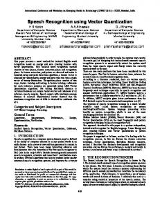
Fig. 1. Example of manual action scenario: a carton of milk is grasped, picked up, and milk is poured into a cup; lower figures show the corresponding visualization of the markers in Nexus [1], a software program from Vicon.

feature vectors to a set of representational codebook vectors c1 , . . . , cK . The codebook vectors are distributed in feature space in a training step by one of the techniques described below. After training, new feature sequences are quantized by computing the closest codebook vector for each feature vector. This can be interpreted as translating the high-dimensional sequences of feature vectors into strings over the finite alphabet of codebook vectors. Quantization is an essential part of our approach since it allows for faster computation in the following matching procedure. We also assume that a VQ algorithm allows for a smoother quantization than dividing the feature space into grids or distributing codebook vectors equidistantly. Instead, VQ algorithms adapt to the data and therefore capture the intrinsic structure of the data. We make use of three approximation techniques to distribute the codebook vectors in feature space. K-means clustering [10] minimizes the distances between K codebook vectors and all samples in training set T by iteratively repeating two steps. The first step assigns each data sample xi to the closest codebook vector cj , and the next step computes a new codebook vector as the average of all assigned data samples. Similarly, SOMs [8] distribute K neurons in the data space. Here, codebook vectors cj are neural weight vectors wi . In the training phase, for each data sample xi , the closest neural weight vector wj is computed and its weights as well as the weights wk of the neighbor neurons are pulled into the direction of xi by w0k = wk + η · h(wj , wk ) · (x − wk ), where η is the learning rate and h is the neighborhood function that defines the distance to the weight vector wj of the winner neuron on the map of neurons. This map is an artificial topology of neurons, typically arranged as a chain or on a grid. The growing neural gas (GNG) by Martinetz [11] is closely related to the SOM, but defines the neighborhood h(·) in data space. Our program is written in Python using the GNG implementation given in the Modular toolkit for Data Processing (MDP) v2.5 [16], a K-means implementation given in SciPy [6] (module scipy.cluster.vq), and our own SOM implementation. 3.4

Dynamic Time Warping

DTW can be used to compute a distance between two sequences s and t of length n and m that are mostly the same but differ by local time distortions. DTW was initially developed for the task of speech recognition, but has since been applied to many domains in which multidimensional linear sequences are observed. The problem is to find a correspondence of each sequence element si of s to an element tj of t and vice versa such that the (weighted) sum of distances between corresponding elements is minimized. This sum is the DTW distance. Since the sequences represent time series data, the correspondences must be monotonic. For example, when si corresponds to tj , then si+1 must correspond to a tj 0 where j 0 ≥ j. We first define a distance d(i, j) between single sequence elements: For Kmeans and the GNG, d(i, j) is the Euclidean distance between the codebook vectors assigned to si and sj . For the SOM, d(i, j) is the distance on the SOM

grid between the two neurons assigned to si and sj . Without VQ, let d(i, j) := ktj − si k. One advantage of using VQ is that we can pre-compute all values of d(i, j), which gives a large speed-up in the following algorithm. To solve the DTW problem, we use this recursion algorithm by Sakoe and Chiba [13]:    g(i − 1, j − 2) + 2d(i, j − 1) + d(i, j),  i = 1, . . . , n, g(i, j) = min g(i − 1, j − 1) + 2d(i, j), , (1)   j = 1, . . . , m g(i − 2, j − 1) + 2d(i − 1, j) + d(i, j) where d(i, j) is a distance between si and tj and g(i, j) is the non-normalized DTW distance between the sequence prefixes s1,...,i and t1,...,j . We let g(i, j) = ∞ when i < 1 or j < 1. g(i, j) can be computed with dynamic programming. The initial condition in Sakoe and Chiba’s paper is g(1, 1) = 2d(i, j), and their normalized DTW distance is DT W (s, t) = g(n,m) n+m . The sequences are therefore compared from end to end. To allow that s may start anywhere within t, we change the initial condition to g(1, j) = 2d(1, j)∀j = 1, . . . , m. To allow 0 ) s to end anywhere, the new DTW distance is DT W 0 (s, t) = g(n,m n+m0 , where 0 0 m = argminj=1,...,m g(n, j). m is the position at which s ends within t. To find out the start position, we introduce table h. If h(i, j) = k, the optimal path through (i, j) starts at position k in sequence t. The initial conditions are h(1, j) = j∀j = 1, . . . , m. h(i, j) is either h(i − 1, j − 2), h(i − 1, j − 1), or h(i − 2, j − 1), depending on which term in (1) is minimal.

4

Experimental Analysis

We now present an experimental evaluation of our approach. We recorded everyday actions similar to the scenario depicted in Fig. 1, which were carried out on four objects (cup, milk carton, pen and book). These recordings serve as reference manual actions and constitute the training data. The actions are: 1) Open book, 2) Pick up pen, 3) Write in the book, 4) Put down the pen, 5) Close book, 6) Pick up milk carton, 7) Simulate pouring milk into cup, 8) Put milk back in original position, 9) Pick up cup and bring to mouth to simulate drinking, 10) Put cup back in original position, and 11) Bring hand back to original position. We then recorded seven long sequences of manual actions that, among other unknown motions, contain variations of the reference actions. The sequences vary in order and orientation to allow an analysis of spatio-temporal dependencies of our technique. For clarity, we illustrate two of the seven sequences: Seq. 1 consists of all the above steps in the order given. In Seq. 5, all four objects were rotated about the z-axis and the cup and the milk carton positions were swapped. The sequence of actions then matched Seq. 1 except that actions 9) and 10) were not carried out. We recorded each sequence three times for a total of 21 sequences. The first seven sequences comprise the validation data and the 14 remaining sequences comprise the test data. The sequences of the validation

data contain 66 known manual actions in total. Those of the test data contain 132 known actions. For all three quantization algorithms, we chose parameters in the following way to limit the codebook size to 100 vectors, which we found to yield a reasonable quantization: For GNG training, we set the maximum number of codebook vectors to 100. We observed that around 70 were used. For K-means clustering, the number of cluster centers was also set to 100. 64 clusters were found to be nonempty. In case of the SOM, we used a 2-dimensional 10 × 10 grid. In this paper, we assume that we know which actions occur in each trial and that each action occurs at most once. This is not an inherent limitation of our approach since preliminary experiments suggest that a properly chosen DTW distance threshold to decide if the action occurs can make the approach fully usable in practice, which will be subject of future work. To measure how well our program finds a gesture, we use the following score function. Let the interval (bp , ep ) be the predicted location of the found action and let (bt , et ) be the true location of the action. We define the (relative) overlap o(bt , et , bp , ep ) := max{min{ep ,et }−max{bp ,bt },0} . The overlap is 100% when both intervals are the max{bp −ep ,bt −et } same and decreases as they move apart. It is zero when the intervals are disjoint. Evaluation Algorithm. A single run of the program consists of the following steps. 1) Load the reference motions; 2) Compute normalized features and train a VQ algorithm; 3) Load either validation or test data and compute normalized features; 4) Convert references and action sequences to symbol sequences using the trained VQ algorithm; 5) For each manual action sequence, search for each known action and record the overlap o; 6) Report the average overlap oˆ and how often o was at least 50%, 75%, and 90%.

4.1

Feature Selection

To find the best feature sets, we ran the program on the validation data using all 29 − 1 possible nonempty feature sets, but without VQ. For each set, we test variance and range normalization and compute features F3–F9 from either all or only the fingertip markers (a total of 4 · (29 − 1) runs). We then looked at the feature sets with the best average overlap oˆ (Tab. 4). All of them contain F1 and F2. F3 was never used and F4 only once. F5–F9 seem to overlap in the sense that at least one of them can be dropped without detriment. For the following experiments, we pick the following feature sets (underlined in Tab. 4). Feature set A is the best in Tab. 4: variance normalization, fingertip markers only, features F1, F2, F5, F6, F8, and F9. Feature set B is at position 5 in Tab. 4 in terms of overlap, but it achieved the highest number of overlaps of at least 90% and contains only four features: variance normalization, all markers, features F1, F2, F8, and F9. Feature set C is at position 15, but also reached a high number of overlaps of at least 90% with only four features: range normalization, all markers, features F1, F2, F6, and F9.

4.2

oˆ [%]

79 . 7866 . 78 3 .0 77 7 . 77 93 . 77 79 . 77 73 . 77 68 .6 77 4 . 77 61 . 77 58 . 77 48 . 77 41 . 77 39 . 7734 . 77 3 .1 77 6 . 77 1 .0 76 8 .9 8

Table 1. Best feature sets among all 2044 possible nonempty feature set/normalization/marker combinations, without VQ. V: Variance normalization; R: Range normalization; T: fingertip markers; A: all markers. The nx rows indicate how often oˆ was at least x% (within 66 actions).

rank norm. markers F1 F2 F3 F4 F5 F6 F7 F8 F9 n90 n75 n50

1 V T × ×

2 V T × ×

3 V A × ×

4 V A × ×

× × × × × × × × × × × 14 13 12 46 44 42 65 64 65

× × × × 14 43 64

5 V A × ×

× × 19 43 64

6 V A × ×

7 V A × ×

8 R A × ×

× × × 12 44 64

× × × × × 10 43 64

× × × × × 14 42 65

9 V T × ×

× × × 16 44 63

10 R T × ×

× × × × × 12 44 63

11 V A × ×

× × 13 43 64

12 V A × ×

13 R A × ×

× × × × × × × × 13 17 44 41 64 65

14 R T × ×

15 R A × ×

× × × 15 44 63

× 21 44 60

16 V A × ×

17 R A × ×

18 V A × ×

19 R A × ×

× × × × × × × × × × × × × × × 18 16 8 12 42 42 45 40 64 61 62 64

Comparison of Vector Quantization Approaches

Using the three chosen feature sets, we ran the evaluation program on the test data set with enabled VQ to compare the approaches in terms of runtime and recognition accuracy (Tab. 4.2).

Table 2. Comparison of K-means, SOM, and GNG recognition accuracy, overall runtime and time spent for DTW, using three feature sets with high recognition rate. Evaluation was done on the test data set. time is total runtime in seconds. DTW is the runtime only for the DTW step in seconds. Feat. set A B C

oˆ [%] 70.35 69.45 64.02

No VQ time DTW 148.2 133.2 151.6 131.8 167.5 147.6

oˆ [%] 68.94 66.76 63.99

GNG time DTW 43.6 17.5 46.5 17.0 44.1 16.4

oˆ [%] 72.23 60.02 62.09

SOM time DTW 231.0 16.3 220.3 16.7 242.7 16.4

K-means oˆ [%] time DTW 70.45 41.0 25.1 66.46 48.0 26.1 63.27 46.7 26.5

The recognition accuracies are almost the same for no VQ, the GNG, and Kmeans. Only the SOM shows slightly worse recognition results for feature sets B and C. We observe significant savings in terms of DTW runtime when the VQ methods are used. The overall runtime is reduced by more than two thirds in the cases of GNG and K-means. In case of the SOM, the increased total runtime is due to a long training time because of the non-optimized implementation.

5

Summary and Outlook

Our experimental analysis reveals that our approach can recognize the manual actions of a small set of everyday actions, while a VQ preprocessing step can lead to significant savings in runtimes. We will extend the approach in various ways. To analyze inter-subject differences, we will enrich the experimental data and record manual actions using different subjects. A further task is to find reliable indicators to decide whether a certain gesture we are looking for occurs at all (in any form). Furthermore, we will extend the framework to a general framework for the recognition of manual action sequences and related multidimensional dynamic data that allows the integration of various preprocessing steps, vector quantization and string matching algorithms.

References 1. Vicon motion capture system. http://www.vicon.com/. 2. G. Caridakis, K. Karpouzis, A. Drosopoulos, and S. Kollias. SOMM: Self organizing Markov map for gesture recognition. Pattern Recogn. Lett., 31(1):52–59, 2009. 3. L. Y. Chang, N. S. Pollard, T. M. Mitchell, and E. P. Xing. Feature selection for grasp recognition from optical markers. In Proc. of the IEEE/RSJ Int. Conf. on Intelligent Robots and Systems, pages 2944–2950, 2007. 4. S. Ekvall and D. Kragic. Grasp recognition for programming by demonstration. In Proc. IEEE Int. Conf. Robotics and Automation, pages 748–753, 2005. 5. D. M. Gavrila and L. S. Davis. 3-D model-based tracking and recognition of human movement. In Proc. Int. Work. on Face and Gesture Recognition, Zurich, Switzerland, 1995. 6. E. Jones, T. Oliphant, P. Peterson, et al. SciPy: Open Source scientific tools for Python, 2001–2010. 7. E. J. Keogh, S. Chu, D. Hart, and M. J. Pazzani. An online algorithm for segmenting time series. In Proc. of the 2001 IEEE Int. Conf. on Data Mining, pages 289–296, 2001. 8. T. Kohonen. The self-organizing map. Proc. IEEE, 78(9):1464–1480, Sept. 1990. 9. H.-K. Lee and J. H. Kim. An HMM-based threshold model approach for gesture recognition. IEEE Trans. Pattern Anal. Mach. Intell., 21:961–973, 1999. 10. S. P. Lloyd. Least squares quantization in PCM. IEEE Trans. Inform. Theor., 28(2):129–137, Mar. 1982. 11. T. Martinetz and K. Schulten. A “neural-gas” network learns topologies. Artificial Neural Networks, pages 397–402, 1991. 12. H. Ritter, H. Robert, F. R¨ othling, and J. J. Steil. Manual intelligence as a Rosetta Stone for robot cognition. ISRR, Dec. 2007. 13. H. Sakoe and S. Chiba. Dynamic programming algorithm optimization for spoken word recognition. IEEE Trans. Acoust. Speech Signal Process., 26:43–49, 1978. 14. T. Stiefmeier and D. Roggen. Gestures are strings: Efficient online gesture spotting and classification using string matching. In Proc. of 2nd Int. Conf. on Body Area Networks (BodyNets), 2007. 15. A. Wendemuth. Grundlagen der stochastischen Sprachverarbeitung. Oldenbourg, 2004. 16. T. Zito, N. Wilbert, L. Wiskott, and P. Berkes. Modular toolkit for Data Processing (MDP): a Python data processing frame work. Frontiers in Neuroinformatics, 2:8, 2008.