Recovering Temporal Integrity with Data Driven Time Synchronization Martin Lukac1† , Paul Davis2† , Robert Clayton3 , Deborah Estrin1† Center For Embedded Networked Sensing† UCLA Computer Science1 UCLA Earth and Space Sciences2 Caltech Division of Geological and Planetary Sciences3 {mlukac,destrin}@cs.ucla.edu,
[email protected],
[email protected]
ABSTRACT
Categories and Subject Descriptors
Data Driven Time Synchronization (DDTS) provides synchronization across sensors by using underlying characteristics of data collected by an embedded sensing system. We apply the concept of Data Driven Time Synchronization through a seismic deployment consisting of 100 seismic sensors to repair data that was not time synchronized correctly. This deployment used GPS for time synchronization but due to system faults common to environmental sensing systems, data was collected with large time offsets. In seismic deployments, offset data is often never used but we show that Data Driven Time Synchronization can recover the synchronization and make the data usable. To implement Data Driven Time Synchronization to repair the time offsets we use microseisms as the underlying characteristics. Microseisms are waves that travel through the earth’s crust and are independent of the seismic events used for the study of the earth’s structure. We have developed a model of microseism propagation through a linear seismic array and use the model to obtain time correction shifts. By simulating time offsets in real data which does not have offsets, we determined that this method is able to repair the offset to less than 0.2 seconds. Our ongoing work will attempt to refine the model to correct the offsets to 0.05 seconds and evaluate how errors in the correction affect seismic results such as event location. Data Driven Time Synchronization may be applicable to other high data rate embedded sensing applications such as acoustic source localization.
C.3 [Special-Purpose and Application-Based Systems]: Real-time and Embedded Systems; J.2 [Physical Sciences and Engineering]: Earth and Atmospheric Sciences
Permission to make digital or hard copies of all or part of this work for personal or classroom use is granted without fee provided that copies are not made or distributed for profit or commercial advantage and that copies bear this notice and the full citation on the first page. To copy otherwise, to republish, to post on servers or to redistribute to lists, requires prior specific permission and/or a fee. IPSN’09, April 13–16, 2009, San Francisco, California, USA. Copyright 2009 ACM 978-1-60558-371-6/09/04 ...$5.00.
General Terms Algorithms, Reliability
Keywords Time Synchronization, Microseisms, Background Noise Correlation
1. INTRODUCTION Time synchronization is a core requirement of embedded sensing applications because the time provides the means to correlate events across sensors. The use of the correlation varies by application but one common use is event source localization. In seismic applications the arrival of events at stations is used for localization of earthquakes. Timing differences in the features of the events such as P-waves and S-waves are used for building models of the crust and mantle (seismic tomography). In existing embedded sensing applications time synchronization is provided by a GPS receiver or by a network time synchronization service. These solutions work well but are not always fault tolerant enough because they are susceptible to poor wireless connectivity, network partitions, start up lag, and unreliable and unpredictable hardware. When such faults occur, the data is deemed unusable. In current practice, if the time synchronization is known to be off for a particular station in a seismic network, the research the data can be used for is limited since there is no good way to consistently recover the data. We propose an approach called Data Driven Time Synchronization (DDTS) to recover data that is com-
promised by time synchronization faults. DDTS uses an underlying characteristic of the data being collected to provide synchronization. The DDTS process builds a model for the characteristic and uses it to compute time correction shifts to apply to the time offset data. We explore DDTS by applying the concept to recently recorded seismic data from the MesoAmerica Subduction Experiment (MASE). These data contain time offsets due to equipment faults. MASE was a joint project between the Center for Embedded Networked Sensing (CENS), the Tectonics Observatory Caltech, and the Universidad Nacional Autonoma de Mexico (UNAM) [9]. The 2 year deployment involved installation of a string of 100 seismic stations seen in Figure 1 stretching 500 km from Acapulco, through Mexico City, to Tampico. Time synchronization was performed by the analog to digital converter (ADC) which converted the GPS signal to a time stamp in the data. As with any deployment, even with this robust hardware, there still were problems: GPS cables were cut and ADCs were misconfigured. These problems combined with transient power failures were exacerbated by a fault in the ADCs which caused large time offsets after a reboot. Up to 7% of the data has time offsets ranging from 10’s of seconds up to 3000 seconds. Figure 2 shows an approximate 260 second time offset discovered for the ZACA station during a local event approximately 140 km South East of the MASE array. We apply DDTS to the time offset data from the MASE deployment. The underlying characteristics used to obtain the time offsets are microseisms: background seismic noise generated by winds in the oceans, which has no correlation to actual seismic events of interest. We have developed a model of the microseism propagation through the MASE seismic array and use it to derive time correction shifts to repair the time offsets to within 0.2 seconds. We apply this to our near-linear array in Mexico. Future work involves extending our approach to areal arrays. Many portable seismic experiments have been conducted in the past with the data stored at the IRIS (Incorporated Research Institutes for Seismology) [1] data center. Most suffer similar loss of time as was experienced in the MASE experiment. Our method could be applied to these data rendering them useful for further analysis. Section 2 introduces Data Driven Time Synchronization and microseisms. Section 3 explains how we detect the time offsets. Section 4 details our model of microseism propagation and the processes of recovering time. In section 5 we evaluate Data Driven Time Synchronization. Sections 6, 7, and 8 discuss the broader applicability of data driven time synchronization, related work, and our future work.
22° N
Huejutla
Pachuca
20° N
Mexico City Cuernavaca
18° N
Acapulco
16° N 100° W
98° W
MÉXICO
20° N
110° W
100° W
90° W
Figure 1: A map of the MASE deployment.
2. DATA DRIVEN TIME SYNCHRONIZATION Data Driven Time Synchronization (DDTS) uses a characteristic of the data collected by the sampling system to recover incorrectly time-synchronized data. The success of DDTS depends on developing a model of a characteristic of the signal to apply to the data to be synchronized. Ideally, there are two requirements of the underlying characteristic for DDTS to be successful. First, the characteristic used is not correlated to the features of the phenomena for which time synchronization is required. Using the same characteristic to resynchronize data and to obtain a scientific result from the data introduces an unacceptable amount of uncertainty. For example, using teleseisms, large distance earthquakes, to resynchronize the data and then using
M 4.1 Event on 2005/10/11,04:17:12.90 −− No Time Correction
BUCU CIEN
Station ID
TOMA TEPO ZACA SATA SAGR MAXE
0
50
100
150
200 250 Time (s)
300
350
400
Figure 2: An example of the time offset experienced at the ZACA station during a local event. 100Hz Vertical Channel Data From Station TONN Frequency Spectrum for 17 Minutes of Data 1 35 30 25 −1 0
20
40
60
Same Data Bandpass Filtered: 0.083 to 0.5 1
Amplitude
Noramlized Amplitude
0
20 15 10
0 5 −1 0
20
40
Time in Seconds
60
0 0
0.1
0.2
Hz
0.3
0.4
Figure 3: 60 seconds of raw unfiltered data and filtered data from MASE. A spectrum of 17 minutes of MASE data. The 6 second microseisms are visible in both the time and frequency domains. the repaired teleseisms to do tomography is undesirable. Second, the characteristic should be either omnipresent or occur at regular intervals such that DDTS can be applied over the entire deployment.
2.1 Microseisms A microseism is a type of seismic wave that is generated by the interference of oceanic surface waves. The interference creates enough pressure on the ocean floor to generate the seismic waves [12] [10]. Microseisms travel through the oceanic and continental crusts. The microseism period depends on the ocean depth and the oceanic surface wave period generated by the wind. Microseisms are omnipresent and exist in the 0.03 to 0.3 Hz frequency range, requiring the use of broadband seismometers. In the MASE data, the dominant period of the microseism energy traveling north through the
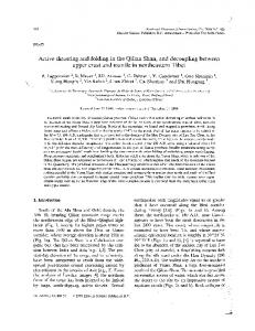
array is 6 seconds, while the dominant period of the microseism energy traveling south through the array is approximately 20 seconds. Figure 3 shows a frequency spectrum of 17 minutes of MASE data (100Hz data filtered and decimated to 1Hz). The approximate 6 second period energy is the peak in the spectrum. Figure 3 also shows the waveform for 60 seconds of 100Hz MASE data, both unfiltered and filtered. The approximate 6 second period microseisms is clearly visible in the filtered data. Microseisms are ideal for applying DDTS because they meet both requirements: they are independent of earthquakes and are omnipresent. Microseisms are not generated by earthquakes and they do not cause earthquakes. This independence makes them ideal for DDTS because it allows earthquakes to be used as the primary means to create models of the crust and the mantle. Like all seismic signals, microseisms can be traced as they travel across a seismic network. The propagation of microseisms between two stations is called travel time. Our goal is to develop a model of the microseism travel time between stations so we can apply DDTS. With a successful model we can predict the travel time for an incorrectly time synchronized station and use that to derive a time correction. Unlike earthquakes, microseisms are continuous and do not have an obvious starting point to try to line up and track the signal across stations. To compute the travel time, we use the lag-time of the peak value of the cross correlation of windows of data from two stations. The lag-time of the peak of the cross correlation is the average travel time of the microseisms over the window. The longer the window of data, the easier it is to determine the peak in the correlogram. Because microseisms are weak, cross correlating very short windows results in correlograms with no clear peak. For our work we use 24 hour windows, which we refer to as short data windows, and 360 day windows which we refer to as long data windows. An example of cross correlating two 360 day windows of data from 2006 is shown in Figure 4. The correlation is from South to North using station EL40 and station TONA. The data was filtered with a bandpass filter around 6 seconds then cross correlated by multiplying spectra obtained using the Fast Fourier Transform (FFT) method. The period of the correlogram shows that there exists a 6 second period oscillation in the signals from both stations. The lag is the amount of time the peak value is offset from zero and gives the time one of the signals must be shifted to best line up with the other signal. The positive lag indicates this energy is traveling North, through EL40 to TONAa. Surface wave energy travels at the group velocity which is different from the phase velocity of the oscillations.
Normalized Amplitude
1
TEMP CANT CIRI RODE ELPA TIBL HUEJ
North
360 day Cross correlation of EL40 to TONA 1.5 Correlogram Group/Envelope Phase Peak Group Peak
IXCA CHIO TLAL OCOL PEMU MOLA TIAN MOJO SAME VENA AGBE NOGA SABI ATOT VEGU SAPA PACH PASU
0.5
0
SAPE KM67 PSIQ ECID TIZA SNLU
−0.5 PTRP ESTA MIXC TEPE
−1 35.90 s
80
The correlogram has two peaks from which we can calculate the corresponding travel times. The travel time of the group peak is the lag-time of the peak of the envelope of the correlogram. The envelope is the overall shape defined by the amplitude of the signal and is the dashed line in Figure 4. The group velocity of the microseisms is determined by the time of the group peak divided into the distance between the stations. The group velocity of the microseisms is around 2.5 km/s. The phase peak is the peak of any one of the oscillations in the correlogram. The phase velocity of the microseisms is determined by the time of the phase peak divided into the distance between the stations. For the 6 second period phase the velocity is around 3 km/s. The position of a specific phase peak depends on the distance between the stations, so when we look at any pair of stations we have to take care in choosing the correct phase peak. For DDTS and our data, we use the phase velocity since in our experience, the group velocities are more scattered and inconsistent between stations. We can also cross correlate across the entire MASE array, both North to South and South to North and see microseisms traveling both directions. Figure 5 shows the North to South cross correlation of all the stations against the TEMP station in the North using 360 days of data. Beacuse we cross correlated from the North to South, the 6 second period North traveling microseisms show up with a negative lag and the 20 second period
PLLI VEVI HUIT PLAT ZURI UICA PETA MAZA PABL ACAH RIVI CARR TICO XOLA PLAY
256
192
128
64
0
EL40 EL30 CEME QUEM ACAP
−64
Figure 4: The results of cross correlating 360 days of data from stations EL40 and TONA. The envelope of the correlogram is the dashed line. The group peak is the peak in the envelope. Its lag-time is used to determine group velocity. Phase velocity, which we use, is determined from the lag-time of a particular phase of the oscillations. We use the peak of the oscillations as a reference phase.
TEPO SATA SAGR TONA MAXE XALI
−128
60
−192
20 40 Lags in Seconds
South
0
−256
−1.5 −20
CHIC PTCU CUCE JIUT TEMI ATLA SJVH PUIX AMAC CASA SAFE PALM BUCU CIEN
Lag in Seconds
Figure 5: The correlograms for a North to South cross correlation sourced at station TEMP. Both the approximately 6 second period South to North moving microseisms and the approximately 20 second period North to South microseisms are visible. South traveling microseisms show up with a positive lag.
3. IDENTIFYING TIME OFFSETS There were a total of 100 seismic stations in the MASE array. 50 of the stations were managed by CENS and 50 stations were managed by Caltech. The CENS stations deliver data through a wireless ad-hoc network and consisted of a broadband Guralp T3 seismometer, an analog to digital convertor (ADC), a CENS station a communications controller, and supporting power equipment [9]. The Caltech stations used Guralp seismometers, data loggers, ADC’s, and supporting power equipment. Time synchronization was performed by the built in GPS receiver on the ADC: a RefTek 130 on the Caltech stations and a Kinemetrics Q330 on the CENS stations. The pulse per second signal and time stamp provided by the GPS receiver are extremely accurate and are used to adjust the internal clock on the ADC. Without a GPS signal the ADC internal clock only drifts a few seconds a month [11], but even this small offset can render the data unusable.
Lags (s) -100
-50
0
50
100
April through May Travel Times
150
200
250
60
300
0 10 15
Day
20 25
Travel Time in Seconds
5
59
58
57
56
30 55
Figure 6: The correlograms for daily cross correlations between CASA and ZACA in the MASE network for the second half of September and the first half of October 2005. The station lost track of time during September 27, 2005 and we can see this as a shift in the correlograms.
As mentioned previously, cut GPS cables and misconfigured ADCs combined with transient power failures caused the large time offsets after a reboot. These are problems that are inherent to these types of systems. 18 CENS stations and 5 Caltech stations experienced the offset. The offsets were always negative (delayed) and averaged less than 1000 seconds. They ranged from 10’s of seconds up to 3000 seconds. To determine how much data was incorrectly time synchronized we used the travel time of microseisms. The velocity of the microseisms through the crust is approximately 3 km/s and the distance between all the stations is known. First we selected stations in our network and from the permanent SSN network [3] which we know have no timing issues and have a nearly complete a record. We know these stations do not have time synchronization problems because they have a GPS log showing multiple active GPS locks for every day. For each day we cross correlated the reference stations with each of the stations in the MASE network and obtained the travel time from the phase peak. Using the known distance between stations and the phase velocity of 3 km/s, we can determine the expected travel time. If the computed travel time from the cross correlation is more than a second or two off the expected travel time, then we know there is a time offset. Figure 6 is an example of the final step in this process for a pair of stations. It shows the daily cross correlations between CASA and ZACA in the MASE network for the end of September and the beginning of October 2005. CASA is a station with good time synchronization. The stations are 38.6 km apart so the travel time is approximately 12 seconds. The x-axis shows the lag
TONA−PTRP 54
0
10
PLAM−PSIQ 20
30
CASA−SAPE 40
TEMI−ATOT 50
60
Day
Figure 7: Travel times for April and May 2006 for four station pairs. The ∗’s represent the calculated travel times and the lines are the travel times generated by Equation 1. The RMSE for each station pair is approximately 0.05 seconds. of the cross correlation. The y-axis represents each day where day 0 is September 16th, 2005. There is a shift in the travel time from minus 12 seconds to 250 seconds during September 27th, 2005. This indicates the station rebooted and lost track of time. During the processes of identifying incorrectly time synchronized stations, we can also identify drift. We can fit a line to the phase peaks across multiple days of offset data. If the line has a significant slope over the course of a month, then the station is potentially drifting. For example by fitting a line to the phase peaks of the offset data in Figure 6, we know there is an approximate 2 second drift over the course of October 2005. For stations which have a more dramatic drift, it is easy to visually identify the drift in the correlograms. Using this method we calculated that almost 7% of the 59,633 station-days in the MASE dataset have time synchronization errors.
4. RECOVERING TIME The first version of our model assumed that the travel time of the microseisms determined from the correlations would be constant in time and not change from one day to the next. Although this is true to within one or two seconds, coherent fluctuations occur across the network, presumed to be caused by changing patterns in the microseisms source. Our current model of microseisms propagation with which we apply DDTS is based on this new observation. We discovered that the time series of daily travel times between pairs of stations fluc-
tuates by up to two seconds but are correlated with one another across independent pairs of nearly aligned (510 degrees apart) stations. The structure of the crust is different between all the stations of the network so the velocity of the microseisms is also different between different pairs of stations. However it is expected to remain constant in time. The fluctuating travel time is not visible in Figure 6 due to scale, but a two month stretch of travel times for four station pairs can be seen as the *’s in Figure 7. So we were left with two questions: why are the travel times fluctuating and why are they correlated between pairs of nearly aligned stations? We have concluded that the fluctuations in the travel times are to due the changing nature of the microseisms. Microseisms are ultimately dependent on the weather so the apparent source of microseisms changes over time. The opposing surface waves that generate microseisms are created by the wind. Patterns of where and when the opposing surface waves generate microseisms constantly shift around due to variations in the weather. There is also not just one source for the microseisms: there are many sources that are changing all the time. The multiple changing random sources are introducing a bias into the signal and causing the fluctuating travel time. Being able to correlate the fluctuations in the travel time between different pairs of stations suggests that there is a common bias in the arriving energy. The bias in the sources must be in the far-field because it is commonmode across the array. Theoretical work [15] has shown that if there are multiple random sources of a signal, only those sources along the receiver line (the straight line joining and extending beyond the stations) stack constructively in the cross correlation as seen in Figure 9. According to theory, when we cross correlate the signals of station A and station B, if the off-receiver line sources are random, they will cancel out and only the energy generated along the receiver line and within the Fresnel zone of the two stations contributes to the cross correlation. In this case, the travel time computed from the cross correlation represents the straight line time between the stations. However, if the pattern of microseism sources on either side of the receiver line is non-random, then from one day to the next, the travel times do not represent the straight line time between the stations. This explains the fluctuating travel time: the sources of microseisms over the short daily cross correlation windows are biased to one side or the other side of the receiver line. This also implies that with a large cross correlation window the microseism sources are more likely to appear random and the bias will be canceled out.
4.1 Microseism Model To repair time offsets and drift we have developed a
Bias
Receiver line Station A
dA,B
Station B
Figure 8: For large cross correlation windows the bias microseism sources cancel out and only the sources along the receiver line stack constructively. For small cross correlation windows, the bias sources become non random and change the phase of the microseisms along the receiver line. model which relates the fluctuations in travel time between multiple pairs of stations and enables us to predict the travel time for the incorrectly time synchronized stations. The model describes the phase change by the biased energy from the off receiver line sources to the averaged microseism energy traveling along the receiver line of two stations. d d d (1) tt = − S + S cos(Z − θ) + f v v v The values tt, d, v, and Z are the travel time, distance, seismic velocity, and angle between two stations. These values are all constants or can be computed using cross correlation. The remaining parameters S, θ, and f represent the strength, S, of the bias field treated as an incident plane wave with angle θ and with f an offset term. They are unknown and are dependent on the particular station pairs and the days we are looking at. We can solve for S, θ, and f as follows. Suppose we have 4 station pairs with 10 days of well correlated travel times for the station pairs. We will be solving for a total of 24 unknowns: an unknown S1 ...S10 for each day, an unknown θ1 ...θ10 for each day, and an unknown offset parameter for each station pair f1 ...f4 . We input the travel times, distances, velocities, and angles between all the station pairs into Equation 1 for a total of 40 equations. This gives us an over determined system of equations we can solve with non-linear least squares.
4.2 Time Correction Process The process to correct the time on an offset or a drifting station has 8 steps. The main idea behind the processes is to obtain parameters for the model about the daily travel time fluctuations using correctly time synchronized data and to use those parameters to predict the travel time for the stations with bad data. Before we perform any cross correlations in the processes, the data is filtered with a bandpass filter around 6 seconds. The data is conditioned with the sign bit method to
remove any high amplitude events, for example earthquakes, that can affect the cross correlation.1 Finally the cross correlation is computed using the FFT method and all the travel times are computed from the phase peak. We have tried various cross correlation window sizes to track the travel time fluctuations and have been most satisfied with a 24 hour window size: it provides the best balance of not averaging out the off receiver line microseisms source bias and providing an easily pickable consistent travel time peak from the cross correlation. 1. Identify the broken stations. We follow the process described in Section 3 to identify the offset and drifting stations. Briefly, we calculate the travel time between a known good station and all the other station. Any travel time which is not within the expected 3 km/s means the station has offset time. This step only needs to be performed once. 2. Calculate the absolute velocities. Our model requires the true velocity between stations. As was discussed earlier in Section 4, short cross correlation windows do not provide a good estimate because the bias in the microseisms sources affects the travel time. To resolve this we calculate the velocity using cross correlation windows that are as large as possible: 360 days and larger. The larger window means that over that longer period of time all the normally non-random microseism sources that introduce bias into the signal do appear random and do cancel each other out. The result is a single velocity for the station pair which is a reasonable estimate of the true velocity. This step only needs to be performed once. 3. Select good data. We select a station and window of data we want to resynchronize. We call the station we want to resynchronize the resync station and the data window we want to resynchronize for that station the resync window. For the resync station we need to select a segment of good data as close to the incorrectly synchronized data as possible. The segment should be about a month of data that does not have any time synchronization issues. We call this segment of data the synced data and use it with other stations in the next two steps to obtain parameters for the model. We run a daily cross correlation over the synced data and the resync window for all station pairs and pick the correct phase peak taking care to avoid cycle skips by using tt estimated from step 2. 4. Select highly correlated stations. Using the resync station we select a couple (3 to 6) station pairs (one of the pairs must include the resync station), for which the travel times correlate well. In other words, for the month of good data, we find station pairs where the fluc1 The sign bit method rewrites the data, setting any sample greater than zero to one, and any values less than zero to zero.
tuations of the daily travel times follow the same pattern and one of these station pairs must be the resync station. These station pairs are easy to find by correlating the time series of the daily travel times and finding independent pairs which have a correlation value of 0.9 or greater. There are some limitations described in Section 4.3. We use these station pairs in the next step to find the offset parameter for the resync station. 5. Solve the model for offset parameter. Next we solve the model as described in Section 4.1 using the synced data and the station pairs from the previous step. We store the offset parameter for the station pair which includes the resync station. We will call this offset fg for the good offset. 6. Solve the model for remaining parameters. Finally, we solve the model as described in Section 4.1, except this time we use the data from the resync window excluding the station pair with the resync station. This step gives us daily S and θ parameters since we did not include any of the incorrectly time synchronized data. We will refer to these parameters as Sg and θg . 7. Calculate correct travel times. Using fg , Sg , θg , the distance, velocity, and angle for the station pair including the resync station, we calculate the travel time for the resync window for the resync station. We call this the predicted travel time. 8. Subtract to get time correction shift and apply. We use the predicted travel time and the offset travel time to obtain the correction shift. For each day, we now have a value to shift all the data by to make that day be the average.
4.2.1 Drift Our method transparently corrects any drift. The predicted travel time is entirely independent from the broken data so for each day we are shifting from the offset and drifted travel time to the predicted travel time. Since the predicted travel time follows the commonmode variation which does not contain any drift our time corrects are compensating for the drift. We initially believed we could correct for drift before the entire processes by using least squares to fit a line to the travel times. However, we found situations where over the course of a month, the drift changes a number of times. This means we have no way to tell whether what we think is drift is actually drift and not just a trend in the data. Beacuse of these cases our method is the ideal solution.
4.2.2 Applying the Corrections The raw data from the MASE deployment is stored on a server and is made available through the Seismogram Transfer Program (STP) [2]. This program supports on-the-fly time corrections based on the corrections es-
2
1
Identify broken stations
Calculate absolute velocities Vi
Daily XCorr to reference station
360 day cross correlation (XCorr)
Badly timed data
Vi
6
Apply model to bad data window Daily Xcorr All stations to all
3,4,5
Apply model to good data Daily Xcorr All stations to all
Obtain common mode variation params S and ș
Solve for offset param f
S,ș
f
7,8
Predict travel time for badly timed data using S, ș, and f Linearly interpolate daily average corrections to digitization interval
Figure 9: A diagram for our method. Not complete yet. There will be numbers on each of the boxes coordinating them with the steps.
timated as described in this paper. The time corrections are stored in a table with columns start date, start time offset, end date, and end time offset. Correction within the start/end dates are derived by linear interpolation. In Section 2.1 we explained that the travel time calculated from the daily cross correlation represents the average travel time of the microseisms between the stations for that day. For this reason we set the time corrections as the middle of the day and let the server interpolate across the corrections. For example, if our method specifies that for 2005/10/10 we add -266.2 seconds, on 2005/10/11 we correct by -266.0 seconds, and on 2005/10/12 we correct by -266.1 seconds, we specify two time corrections as shown in Table 1. For the beginning edge cases we extrapolate back using the subsequent corrections and for the ending edge cases we extrapolate forward using the preceding corrections.
4.3 Model Limitations There are three limitations to our method. First, the station pair selection process reveals some limiting factors of the model and of this particular application of DDTS. In order to estimate model parameters, we require good data from the station with the incorrectly
time synchronized data. If during the course of the deployment, if a station never has good data, then we can only estimate the travel time to within a second or two based on the distance between the stations. Some good data must exist because we need an estimate of the offset parameter f in the model and we can only determine f with good data. The second limiting factor is there needs to be at least a few stations pairs that share receiver lines. We have found that station pairs with receiver lines that are farther than 5 to 10 degrees apart tend to not follow the model as well as stations for which the receiver lines are relatively aligned. The sources that are off the receiver line (and outside the Fresnel zone) will average together differently for stations pairs which are not aligned resulting in varied effects on the microseism phase. Choosing aligned stations for the processes ensures there exist stations pairs for which the model does apply and for which the travel time fluctuations follow the same pattern. So far, we have always found there to be some combination of station pairs with valid data that share receiver lines by looking for high correlations of the time series of the travel times of stations pairs. We do expect to find some cases where we are unable to repair the data and in these cases the alternative is to use a less accurate method to obtain a time correction shift. The final limitation is the station pairs need to be more than 50 km apart. For stations which are within 50 km, the travel time computed from the cross correlations can vary by up to 6 seconds. This is because the interference in the correlogram of the North and South traveling microseisms. We can see this interference in the North most stations in Figure 5. It is not possible to differentiate or filter the north moving energy and the south moving energy in the cross correlation for stations within 50 km of each other. The variations in the travel time caused by this interference do not correlate between stations so we are unable to apply our model.
5. EVALUATION To evaluate DDTS in three ways using the actual data collected by the MASE array. First, we show how well the model is able to predict the travel time of the microseisms. Second, we show how the accuracy of the prediction affects the result of a simple local earthquake localization method. The third evaluation is to show our method applied to real time offset data. For the first two evaluation methods, we use good data and introduce an artificial time offset error. This provides us with the ability to compare the data to the ground truth.
5.1 Model Prediction Evaluation Out of the two years of data we focus on March, April, May, and July of 2006. There is an immense amount of
Start time 2005/10/10,12:00:00.00 2005/10/11,12:00:00.00
Offset -266.2 -266.0
End Time 2005/10/11,12:00:00.00 2005/10/12,12:00:00.00
Offset -266.0 -266.1
Table 1: Sample time correction to the MASE STP server. data to work with and we feel that these months provide a good cross section of the scenarios we are interested in. We select two months of good data and we run the daily cross correlations for all pairs of stations to obtain the travel times. One of the months is designated as the resync window described in Section 4.2 and a randomly selected station is set as the resync station. We follow the processes to obtain a time correction shift for the resync station as if it was actually offset. Briefly, we obtain fg for the resync station using the first month of data, and obtain the Sg and θg parameters from the second month of data not including the station pair with the resync station when we solve the model. We simulate the time offset by not including the station when we solve the model with the travel times from the resync window. We then compare the predicted travel time for the resync station to the actual travel time for the resync station and compute the RMSE. Finally the whole processes is repeated with a separate set of stations and two different time windows.
5.1.1 Results The results of the evaluation for the model prediction are in Table 2. As described earlier, we select a pair of months such that the first month is used to calculate needed parameters to predict a time offset in the second month. For each pair of months, we randomly select 5 or 6 station pairs according to the criteria described above. We run the model on the first month of travel times to obtain the parameters. We then run the model on the second month of travel times, minus one of the station pairs, to obtain the final parameters. Combining the parameters from both months, we predict the travel time for the station pair removed from the second month and compare the result to the actual travel times for that station. We then compute the RMSE of the prediction. This processes is done 10 times for each pair of months, each time using station pairs that have not been used before. The results in the right most column in the table are the mean and standard deviation of the 10 RMSE calculations for each month pair. We are able to predict the travel time for the station with the simulated offset to within 0.2 seconds. The table also shows the mean RMSE for how well the model was able to fit the data from the first month: the month used to determine the offset parameter. This was also averaged across the selection of 10 stations.
The RMSE of the model fit is within 0.1 seconds.
5.2 Local Earthquake Localization We have determined that we can repair the time offsets to within 0.2 seconds, but still leaves us with the question of whether the 0.2 second accuracy is good enough to be able to the data within the broader science processes. To answer this question we perform a simple sensitivity analysis within the context of our deployment on the processes of localization of local earthquakes. We use local earthquakes recorded by the MASE array and compute how different time offsets affect the localization result in terms of distance from the real hypocenter (the x, y, and z location of the earthquake). We localize an earthquake by using multilateration. This processes is straightforward: we choose the arrival times of the pwaves and the locations of the stations to solve for the hypocenter using non linear least squares. We have chosen two local earthquakes as examples both located in the South of the array: the first occurred on April 1, 2007 at 22:25 GMT and the second occurred on January 13, 2007 at 02:25 GMT. After computing the hypocenter using 9 stations for each of the earthquakes, we choose the closest station to each of the quakes and offset the time from -3 second to 3 second in 0.1 second increments. The selected results of this processes are in Table 3. At +-1 second the hypocenter of the first earthquake is already greater than 30 km away from the true hypocenter for that earthquake. Figure 10 shows a three dimensional view of the stations, the true hypocenter, and the hypocenter location for +-1 second offsets in 0.1 increments. Temporary arrays such as MASE are expected to be able to localize local events to within 1 km horizontally and 3 km vertically. Table 3 shows that this expected accuracy is not achieved once the time offsets are greater than 0.1 seconds for the April 2007 event and greater then 0.2 seconds for the January 2007 event. This means that our method is correcting the time offsets to right around the accepted accuracy.
5.3 Real Data Repair For our final evaluation we repair a real offset and drift in data from the MASE deployment. We selected September and October of 2005 and identified the station ZACA as having incorrect time synchronization using the method described in Section 3. Figure 6 shows that on September 27th, 2005 the station can see the
Month Pair March-April May-July March-July
First ’good’ month mean/stddev of the RMSE for the entire model fit 0.073 / 0.006 0.075 / 0.009 0.077 / 0.013
Mean/stddev of the RMSE of the predicted travel times 0.115 / 0.028 0.126 / 0.028 0.142 / 0.024
Table 2: The first column is the mean/standard deviation of the RMSE across 10 runs for the first month of ’good’ travel times. The second column is the mean/standard deviation of the RMSE across 10 runs of the predicted travel time for a station pair during the second month. Apr 07 EQ Dist from hypocenter 52.64 55.96 35.49 15.46 6.09 3.04 3.05 6.13 15.63 33.10 81.58 22716.55
Jan 07 EQ Dist from hypocenter 58.37 31.59 14.64 7.14 2.82 1.41 1.40 2.78 6.89 13.62 26.88 68.84
Table 3: Distance in km from the real hypocenter when time offsets are introduced to the station closest to the real hypocenter for two local earthquakes in the Southern portion of the MASE array. data go bad during September 27th, 2005. We apply the processes described in Section 4.2 and update our data server with the time corrections. We then reran the processes used to generate Figure 6 and the results can be see in Figure 11. The time offset is corrected and the drift has been removed. Figure 12 shows the same local event as Figure 2 after our method has been applied to repair the ZACA for October 2005.
6.
BROADER APPLICABILITY
This work can be applied to other seismic deployments, in particular the large catalogs available from IRIS [1]. Time synchronization problems are common enough in these deployments that the possibility of revisiting past experiments and recovering the data is exciting. Our application of DDTS can also be applied as a primary form of time synchronization for ocean bottom seismic arrays. These arrays lack the ability to use GPS for time synchronization and in current practice the clocks are just allowed to drift. In conjunction with coastal seismometers which can maintain time using GPS receivers, microseisms can be used to keep the drift in check: the travel times would appear to be increasing or decreasing over time and our model can be used to repair the drift. It is possible to apply the idea of DDTS to repair time
Earthquake Localization
50
0
Km
Seconds Offset -5.00 -2.00 -1.00 -0.50 -0.20 -0.10 0.10 0.20 0.50 1.00 2.00 5.00
−50
−100
MASE stations Hypocenter with Time Offsets
−150 80
True Hypocenter 60
100 40
50
20 Km
0
0
Km
Figure 10: The effects of +-1 second offset in .1 second increments on an April 2007 earthquake localization with 9 stations in the south of the MASE array. The distance from the real hypocenter at +-1 second is greater than 30 km.
synchronization faults in acoustic source localization applications. These applications typically use direction of arrival (DOA) methods to localize a source [6], [4]. Before these systems can perform source localization they must self localize and determine the location of each of the sensors. The self localization processes requires time synchronization because it uses time of flight in addition to DOA to provide accurate results. If a station is not time synchronized during the self localization it can not participate in the source localization. This is where data driven time synchronization comes in. Since DOA does not require time synchronization, the DOA results from the broken station combined with the DOA results from the working stations from the self localization steps could be used to estimate the position of the broken node. Once the position of the broken node is known, a time offset for the time synchronization can be estimated. The exact processes and whether this can be used to increase the accuracy of the final source
Lags (s) -100
-50
0
50
100
M 4.1 Event on 2005/10/11,04:17:12.90 −− Time Corrected
150
200
250
300
0 BUCU
5 CIEN
10 15
Day
20
Station ID
TOMA TEPO ZACA
25
SATA SAGR
30 MAXE
Figure 11: The correlograms for daily cross correlations between CASA and ZACA in the MASE network for the last half of September and the first half of October 2005 after applying the time correction from our method. See Figure 6 for the daily correlograms before the data was time corrected. localization result remains as future work. We are interested in trying to correlate background noise in acoustic signals in the same we correlate the background seismic noise. We have a number of data sets from past acoustic source localization experiments and plan to explore whether this is possible as future work. DDTS can be applied to environmental sensors as well. Sundial [7] successfully applies the DDTS idea to light sensors tracking solar patterns.
7.
RELATED WORK
The physics behind our model is descried in [15]. Sundial [7] is an independently developed system which implements the DDTS idea for environmental sensors. The work successfully reconstructs time stamps by correlating annual solar patterns with readings from light sensors available on their nodes. 11 years of data from three stations have been studied by Stehly [16] to attempt to detect changes in the travel time of microseisms between the stations due to physical change in the crust. They are unable to detect changes in travel time due to physical change, but identify changes due to clock drift and other instrumental errors. They attempt to separate the offset in time due to clock drift and instrumental errors from the change in the location of the microseism sources. They use a long 6 year period which had no timing errors as a reference and compare to this short 1 month and 6 months windows of data. The comparisons enables them to identify time offsets due to clock drift and instrumental errors and use these to repair the data independent of the travel time. There is no evaluation of how accurate
0
50
100
150
200 250 Time (s)
300
350
400
Figure 12: A local event after the time offset and drift at ZACA has been repaired with out method. See Figure 2 to see the data without the time correction. the results are. The variations in the travel time due to changing microseisms source locations are evident, but the work does not use the microseism variation to resynchronize the data as we do here. There is a growing body of work which uses microseisms for tomography such as [5] and [13]. These study how microseisms can reveal the structure of the crust and attempt to determine if it changes over time. Other work studies microseisms and attempts to locate the origin of dominant sources [10] [14]. Werner-Allen [17] experienced network time synchronization instability and errors during a wireless embedded sensing deployment on a volcano. The errors were due to bugs in the software system and lasted for a few hours at a time. Their approach to detecting and repairing the synchronization problems is not data driven: it does not use the data collected by the sensors in the network. Instead they take advantage of the system itself: as the data streams from the network the base station adds an addition an additional timestamp to the data. They are able to build piecewise linear models between the clocks in the system: base station clock, the global time from the network time synchronization, and the local node time. The models provided a time reference and conversion for the data to be repaired.
8. FUTURE WORK Our primary focus is to increase the accuracy of our methods down toe 0.05 seconds for seismic arrays. This involves exploring various avenues: using higher data rate data such as the real 20 or 100 Hz data, using the North to South 20 second period microseisms, as well as
expanding the model to work for more than just station pairs which have receiver lines within a few degrees of each other. We will also begun correlating microseisms with potential sources such as the wind and the significant wave height models for the oceans. This correlation has the potential of enhancing the model and increasing its accuracy. We believe it is possible to remove the limitation of the linear array. We will investigate the use of the correlation of coda of correlation method for this purpose. We will evaluate the accuracy of our method by comparing the results to a recently developed deep tomography velocity model [8]. This model was built using teleseisms detected by the MASE array and can be used to predict the time the teleseisms should have arrived for the stations with time offsets. We can compare this prediction to the prediction generated by our methods. We will also perform more in depth evaluation on how much of a difference the corrected time and any error introduced with the corrected time has on the science results from the deployment such as the deep tomography velocity model.
[4] A. M. Ali, T. Collier, L. Girod, K. Yao, C. Taylor, and D. T. Blumstein. An empirical study of acoustic source localization. In IPSN ’07, 2007. [5] P. Gerstoft, K. G. Sabra, P. Roux, W. A. Kuperman, and M. C. Fehler. Green’s functions extraction and surface-wave tomography from microseisms in southern california. Geophysics, 71(4):SI23–SI31, 2006. [6] L. Girod, M. Lukac, V. Trifa, and D. Estrin. The design and implementation of a self-calibrating distributed acoustic sensing platform. In ACM SenSys 2006, 2006. [7] J. Gupchup, R. Musaloiu-E., A. Szalay, and A. Terzis. Sundial: Using sunlight to reconstruct global timestamps. In To appear EWSN, 2009. [8] A. Husker. Tomography of the Subducting Cocos Plate in Central Mexico Using Data from the Installation of a Prototype Wireless Seismic Network: Images of a Truncated Slab. PhD thesis, University of California Los Angeles, 2008. [9] A. Husker, I. Stubailo, M. Lukac, V. Naik, R. Guy, P. Davis, and D. Estrin. Wilson: The wirelessly linked seismological network and its 9. CONCLUSION application in the middle american subduction experiment. Seismological Research Letters, 79(3), Data driven time synchronization is a viable time synMay/June 2008. chronization method. We are able to applying the con[10] S. Kedar, M. Longuet-Higgins, F. Webb, cept of DDTS to repair time offset data from the MASE N. Graham, R. Clayton, and C. Jones. The origin deployment data. Our application makes use of a new of deep ocean microseisms in the north atlantic observation about microseisms and models this obserocean. Proceedings of the Royal Society A, vation across a linear array of broadband seismometers. 464(2091):777–793, March 2008. The model is able to predict the travel time of micro[11] Kinemetrics. Q330 clock stability discussion. seisms in a 24 hour period enabling the time offset surPersonal Correspondence, May 2008. rounding seismic events of interest to be repaired. There are limitations to our current implementation, however [12] M. S. Longuet-Higgins. A theory of the origin of the results are good enough to motivate further investimicroseisms. Philosophical Transactions of the gation in other applications. Royal Society A, 234(875):1–35, September 1950. [13] N. M. Shapiro, M. Campillo, L. Stehly, and M. H. Ritzwoller. High-Resolution Surface-Wave 10. ACKNOWLEDGEMENTS Tomography from Ambient Seismic Noise. The MASE array and this work was partially supScience, 307(5715):1615–1618, 2005. ported under NSF Cooperative Agreement #CCR-0120778. [14] N. M. Shapiro, M. H. Ritzwoller, and G. D. The MASE array was partially supported by the GorBensen. Source location of the 26 sec microseism don and Betty Moore Foundation through the Tectonfrom cross-correlations of ambient seismic noise. ics Observatory at Caltech. Contribution number XXX Geophysical Research Letters, 33, 2006. from the Tectonics Observatory. [15] R. Snieder. Extracting the green’s function from the correlation of coda waves: A derivation based 11. REFERENCES on stationary phase. Phys. Rev. E, 69(4):046610, Apr 2004. [1] Incorporated research institutions for seismology. [16] L. Stehly, M. Campillo, and N. M. Shapiro. http://www.iris.edu. Traveltime measurements from noise correlation: [2] Seismogram transfer program (stp). stability and detection of instrumental time-shifts. http://www.data.scec.org/STP/stp.html. Geophysical Journal International, [3] Servicio sismol´ogico nacional (ssn). 171(1):223–230, October 2007. http://www.ssn.unam.mx/.
[17] G. Werner-Allen, K. Lorincz, J. Johnson, J. Lees, and M. Welsh. Fidelity and yield in a volcano monitoring sensor network. In OSDI, November 2006.