Recurrent Memory Array Structures Technical Report
arXiv:1607.03085v2 [cs.LG] 13 Jul 2016
Kamil M Rocki∗ IBM Research, San Jose, 95120, USA (July 14, 2016)
Abstract The following report introduces ideas augmenting standard Long Short Term Memory (LSTM) architecture with multiple memory cells per hidden unit in order to improve its generalization capabilities. It considers both deterministic and stochastic variants of memory operation. It is shown that the nondeterministic Array-LSTM approach improves stateof-the-art performance on character level text prediction achieving 1.402 BPC† on enwik8 dataset. Furthermore, this report estabilishes baseline neural-based results of 1.12 BPC and 1.19 BPC for enwik9 and enwik10 datasets respectively.
1
Background
It has been argued that the ability to compress arbitrary redundant patterns into short, compact representations may require an understanding that is equivalent to general artificial intelligence (MacKay, 2003; Hutter, 2005). One example of such a process is demonstrated by learning to predict text a letter at a time. A strong connection between compression and prediction was shown (Shannon, 1951). Therefore, this report considers experiments on natural wikipedia text corpora, however the algorithms can be in principle applied to any sequences of patterns.
2
Simple RNN
A standard recurrent neural network (so called simple RNN, cite) is composed of a matrix of connections between its inputs and hidden states W , and a matrix U , connecting hidden states in consecutive time steps. In such a simple RNN architecture the entire history of observations in aggregated in hidden states of neurons (fig 2.1). States (ht ) are determined by previous states (ht−1 ) and feedforward immediate inputs (xt ). This architecture is deterministic, for ∗
[email protected] † bits
per character
1
2 identical ht−1 , xt there will be 2 identical outputs ht . A single time step update can be expressed with an equation (1) or equivalently using the following graphical representation as shown in fig. 2.1. ht = tanh(W xt + U ht−1 + b)
...
ht−1 xt
U
ht
tanh
internal state
(2.1)
...
W
Figure 2.1: Simple RNN unit (omitted implementation specifics); ht - internal (hidden) state at time step t; x are inputs, y are optional outputs to be emitted; All connections are learnable parameters. No explicit asynchronous memory, implicit history aggregation only through hidden states h. Omitted bias terms for brevity.
3
Memory structures
A simple RNN architecture does not handle long-range interactions and multiple simultaneous context well (Bengio et al., 1994). However, it can be modified in order to make learning long-term dependencies easier. One solution to the problem is to change the way of interactions between hidden units, i.e. add multiplicative connections (Sutskever et al., 2011). Another is by adding explicit memory cells. Networks involving register-like functionality allowing hidden states to store and load its contents in an asynchronous way have been very successful recently. Examples of such architectures include Long-Short Term Memory (Hochreiter and Schmidhuber, 1997) and Gated Recurrent Unit (GRU) (Chung et al., 2014) networks.
3.1
LSTM
This section describes a standard LSTM network used in our experiments and serving as a foundation for array extensions. Equations 3.1-3.6 define a single LSTM time step update. f t = σ(Wf xt + Uf ht−1 + bf ) t
t−1
+ bi )
(3.2)
t
t
t−1
+ bo )
(3.3)
i = σ(Wi x + Ui h
o = σ(Wo x + Uo h t
(3.1)
t
t
t−1
c˜ = tanh(Wc x + Uc h
+ bc )
ct = ft ct−1 + it c˜t 2
(3.4) (3.5)
...
ct−1
memory lane
.
ft
...
ht−1
it
ot
.
c˜t
control logic
.
...
ct
+
ht
internal state
...
xt Figure 3.1: LSTM, biases and nonlinearites omitted for brevity; The memory content ct is set according to the gates’ activations which are in turn driven by the bottom-up input xt and previous internal state ht−1 . ht = ot tanh(ct )
3.2
(3.6)
State-sharing Memory: Array-LSTM
POTENTIAL SYNAPSE (A BIT LOCATION)
Fig 8. The structure of the cerebellarcortcx of the brain. PU = Purkinje cell (black); Go = Golgi cell (dotted);GI = granule cell; Pa = parallel fiber: St = stellate cell; Ba = basket cell; C1= climbing fiber; Mo = mossy fiber (black) (From"The Cortex of the Cerebellum",by R. Llinas, Copyright 0 1975 by Scientific American, Inc. All rights reserved.)
Fig 9. Simplified structure for the ccrebcllarcortcx of the brain.
Even more provocative is the manner in which the climbing fiber branches to follow the dendritic tree of a Purkinje cell to its synapses with the parallel fibers. In 1970, David M m proposed that the function of the cerebellum is pattern leaming.6 Marr postulated that the firing of the climbing fiber, coincident with the activation of parallel fibers, caused changes in the Purkinje-cell-parallel-fiber synapse which facilitated future firings across those synapses. James Albus, and, later, Pentti Kanerva, independently proposed similar models for the cerebellum. 2*7*8 These models are now recognized as essentially equivalent. I will refer to this model as the Marr-Albus-Kanerva (or MAK) model of the cerebellum. Of interest in this paper is the relationship of the MAK model of the cerebellum to the sparse distributed memory algorithm. This is best described using the simplified model of the cerebellum shown in Figure 9. (For simplicity, the Golgi, basket, and stellate cells have been left out of the figure.) In this proposed relationship, the mossy fibers are transmitting the reference address for the memory. Each granule cell is
acting as a memory location; it only fires when the address transmitted along the mossy fibers is close enough to the address it represents. Thefiring of u granule cell can be considered equivalent to the selection of (I location in the SDM model. (The Golgi cells, which are not shown in our simplified drawing, may be involved in setting the radius for the memory.) A major question is the site in the cerebellum corresponding to the data counters in SDM. Kanerva postulates that the data counters are the synapse points wheFe parallel fibers, climbing fibers, and Purlunje cell dendrites meet. This is the same location where Marr postulated learning to take place in the system. If this hypothesis about these synapses is correct, then the c h b i n g fibers could be carrying the input data for the memory. This would explain the careful construction of the cerebellum, where each Purkinje cells receives input from exactly one climbing fiber. The Purkinje cells provide the output data from the system. As the natural function of a neuron is to sum its inputs and fire if over threshold, they would serve admirably in this capacity and mirror the functioning of a column in a SDM (see Fig. 5). While this correspondence is suggestive, there is little direct evidence to support it. Even 18 years after Marr suggested a site for plasticity in the cerebellum. there is still a Lively debate among neuroscientists as to whether this plasticity
Figure 3.2: The structure of the cerebellar cortex (Kanerva, 1988)
Cerebellar cortex structure as described in (Kanerva, 1988) among others: Fig. 3.2 shows array-like structure in what seems to be Random-Access Memory in cerebellum. It has served as an inspiration for the Array-LSTM architecture. The main idea is that instead of building hierarchies of layers (as in stacked LSTM (Graves, 2013), Gated-Feedback RNN (Chung et al., 2015)) keep a single layer, but build more complex memory structures inside a RNN unit 3
memory lanes
...
ct−1 3
.
+
ct3
...
...
ct−1 2
.
+
ct2
...
...
ct−1 1
.
+
ct1
...
...
ct−1 0
.
+
ct0
...
. . .
it3
ot3
it2
ot2
it1
ot1
it0
ot0
control logic
.
. . . . P
f3t
...
ht−1
f2t
f1t
f0t
c˜t3
c˜t2
c˜t1
c˜t0
ht
internal state
...
xt Figure 3.3: Array-LSTM with 4 memory cells per hidden control unit; modulated vs modulating connections, omitted nonlinearities and biases for brevity; It becomes a standard LSTM when only 1 memory cell per hidden unit is present (a similar line of thinking has been explored by contructing a more complex transition function inside a layer (Pascanu et al., 2014)). We want to create a bottleneck by sharing internal states, forcing the learning procedure to pool similar or interchangeable content using memory cells belonging to one hidden unit (analogy would be that a word related to car would activate a particular hidden state and each memory cell could be interchangeably used if it represents a particular car type, therefore externally the choice of a particular memory cell would not be relevant. Similar concepts exist already in convnets, i.e. spatial pooling, the hidden state should work as a complex cell pooling multiple possible substates. Figure 3.3 and equations 3.1-3.6 describe a single Array-LSTM architecture. Note the similarity between figures 3.2 and 3.3. Furthermore, We consider modifications of the presented simple Array-LSTM architecture which are meant to improve capacity, memory efficiency, learning time or generalization. This report shows two types of changes, one pertains to deterministic family of architectures and the other one to stochastic operations (working in a dropout-like fashion). fkt = σ(Wf k xt + Uf k ht−1 + bf k )
(3.7)
itk = σ(Wik xt + Uik ht−1 + bik )
(3.8)
4
otk = σ(Wok xt + Uok ht−1 + bok )
(3.9)
c˜tk = tanh(Wck xt + Uck ht−1 + bck )
(3.10)
ct−1 k
c˜tk
(3.11)
otk tanh(ctk )
(3.12)
ctk
=
fkt
ht =
X
+
itk
k
4
Deterministic Array-LSTM extensions
4.1
Lane selection: Soft attention
We allow hidden state to choose a memory cell that it wants to read from and write to. This choice will be invisible to other hidden states, so that multiple memory cell choices can be mapped to the same internal state, giving some space to learning invariant temporal patterns. Compared to the original LSTM and simple Array-LSTM, one additional gate activation per memory lane is computed. We call it selection gate. See Fig. 4.1 and equations (4.1-4.8) for details. The intuition behind this approach is that the s gates control how much a particular memory lane should be used during current time step. If st is 1 then all other activations remain unchanged, we fully process this memory cell. If st is 0, then the contents are carried over from the previous time step and the memory cell is not affected during that time step (no read/no write). The idea is that such a mechanism should allow less leaky memory cells, effectively not relying entirely on forget gate in order to preserve its contents. Each memory lane has a selection gate st associated with it, controlling information flow through or bypassing current time step (carrying over memory content from previous time step). The idea is that s gates should be responsible for controlling the timescale (as proposed in the Zoneout paper (Krueger et al., 2016)). Attention signals k. atk = σ(Wak xt + Uak ht−1 + bak )
(4.1)
Softmax normalization. t
eak stk = P at k ke
(4.2)
fkt = stk σ(Wf k xt + Uf k ht−1 + bf k ) itk otk
=
stk
=
stk
(4.3)
t
t−1
+ bik )
(4.4)
t
t−1
+ bok )
(4.5)
σ(Wik x + Uik h
σ(Wok x + Uok h
c˜tk is not affected by stk . c˜tk = tanh(Wck xt + Uck ht−1 + bck ) 5
(4.6)
1-st3
.
...
ct−1 3
st3
˜
.
st3
memory lanes
.
+
ct3
...
.
+
ct2
...
.
+
ct1
...
.
+
ct0
...
1-st2
.
...
ct−1 2
st2
˜
.
st2
1-st1
.
...
ct−1 1
st1
˜
.
st1
1-st0
.
...
ct−1 0
st0
˜
.
attention
st0
internal state / control logic
Figure 4.1: Lane selection through soft attention, solid lines are control logic signals (from/to gates), dotted lines are memory cell lanes used upon selection, dashed lines represent the carry lanes used otherwise; dotted and dashed lanes are mutally exclusive Note the inverted f gate effect for clearer notation (cell k is reset for fk = 1). If stk is 0, then fkt is 0 and effectively k memory cell’s contents are entirely transferred for the previous time step. ctk = (1 − fkt ) ct−1 + itk c˜tk k ht =
X
otk tanh(ctk )
(4.7) (4.8)
k
Max pooling version In this version the algorithm used a hard, deterministic selection, by choosing the lane with highest st value. It ignores other lanes and backpropagates errors only through that lane, It is analogous to max pooling in CNNs.
5 5.1
Non-deterministic Array-LSTM extensions Stochastic Output Pooling
This is the simplest of the considered stochastic architectures (Fig. 5.1). It works by treating initial o gate activations as inputs to a softmax output distribution and sampling from this distibution. Therefore it enforces normalization of output response and sparse binary outputs (6 1/2). During backpropagation, the algorithm uses only the selected gate (as in the max attention algorithm in 4.1). All other steps are exactly the same as the standard Array-LSTM approach in 3.2. Probability that memory cell i will used during ht update (other cells’ outputs are not used): 6
ct0
discretize
softmax
ot1
ct2
ct3 .
ot3 ot2
ct1
. . .
ot0
P
ht
Figure 5.1: Stochastic Output Pooling: Sample open output gate index i from this distribution calculated using sof tmax normalization. Dotted lines represent inactive connections (set to zero due to the sampling procedure).
memory lanes
...
ct−1 3
.
+
ct3
...
...
ct−1 2
.
+
ct2
...
...
ct−1 1
.
+
ct1
...
...
ct−1 0
.
+
ct0
...
internal state / control logic Figure 5.2: Stochastic Memory Array: solid lines are control logic signals (from/to gates), dotted lines are memory cell lanes used upon selection, dashed lines represent the carry lanes used otherwise; dotted and dashed lanes are mutally exclusive
t
eok p(i = k) = P ot k ke
(5.1)
The hidden state ht is computed using the active output cell index. ht = oti tanh(cti )
5.2
(5.2)
Stochastic Memory Array
This is a more complex architecture, an active cell is being chosen for the entire cycle of computation. Instead of selecting only the output memory cell, the algorithm chooses one memory lane to be used during the entire forward and backward loop. If a lane is not selected, carry over cell contents. This idea is very similar to the algorithm described as Zoneout (Krueger et al., 2016). The main difference between two implementations is the fact that here, the hidden state is not affected directly by the noise injecting procedure. Instead, by choosing 7
exactly one memory lane, it ensures that the output of the memory is non-zero and the content of ht is going to be non-zero (I found that the main instability of all stochastic approaches, including Recurrent Dropout (Zaremba et al., 2014) is caused by the fact that all or almost all hidden states’ activations can be zeros. Figure 5.2 depicts the changes to the original Array-LSTM architecture from 3.2. Each memory lane has an additional bypass connection which is used when memory cell is not selected for computation (as in the soft attention algorithm in 4.1). We consider 2 variants of this approach: (a) 1 out of K cells is active (b) 1/2 cells are active, i.e. 4 out of 8. In the first implmentation, the algorithm randomly chooses index of the memory cell to be used. In the latter one, the same procedure applies, only to groups of 2 cells (odd or even). 5.2.1
Stochastic hard attention
Here this report describes different implementations of combinining the soft attention mechanism with stochastic lane selection. We would like to select memory cell in a semi-random way, according to some selection distribution as described in 4.1. Semi-Hard One memory lane is selected as being active (as in Stochastic Memory Array from 5.2). However, unlike the previous fully random selection mechanism, in this approach the lane is selected according to softmax distribution where s are inputs controlling this distribution. The backward step is the same as in the soft attention version, ignoring the fact that in the forward pass a sample was used and computes derivatives using differentiable softmax outputs. Hard 5.2)
5.3
Same as v1, but the backward pass uses only the selected lane (as in
Implementation considerations
Array-LSTM brings many advantages from the computation cost perspective. 1. More memory cells Given the same amount of memory for allocation, Array-LSTM has effectively use more memory cells due to smaller matrix between hidden units and gates. 2. More parallelism More cells give raise to more independent elementwise computation which is very cheap on SIMD hardware like GPUs. 3. More data locality Cells belonging to the same hidden unit will be somehow correlated which might improve cache hit ratio. In addition to that, sparse hidden to hidden connectivity might be possible for larger number of cells per unit. 4. Approximate Stochastic Array Memory is naturally resilient to noisy input. 8
6
Related Works
There are many other approaches to improving baseline LSTM architecture including deterministic approaches such as Depth gated LSTM (Yao et al., 2015), Grid LSTM (Kalchbrenner et al., 2015) or Adaptive Computation Time (Graves, 2016). Examples of stochastic variants include recurrent dropout (Zaremba et al., 2014; Semeniuta et al., 2016) Batch normalization (Cooijmans et al., 2016) and Zoneout (Krueger et al., 2016).
7
Experiments
7.1
Methodology
The learning algorithm used was backprogagation through time (BPTT), it proceeded by selecting random sequences of length 10000 randomly from a given corpus. The learning algorithm used was Adagrad‡ with a learning rate of 0.001. Weights were initialize using so-called Xavier initialization Glorot and Bengio (2010). Sequence length for BPTT was 75 and batch size 128, states were carried over for the entire sequence of 10000 simulating full BPTT. Forget bias was set initially to 1. These values were not tuned, so it is possible that better results can be easily obtained with different settings. The algorithm was written in C++ and CUDA 8 and ran on GTX Titan GPU for up to 20 days. Link to the code is at the end.
7.2
Data
7.2.1
enwik8
It constitutes first 108 bytes of English Wikipedia dump (with all extra symbols present in xml), also known as Hutter Prize challenge dataset∗ . 7.2.2
enwik9
This dataset is used in Large Text Compression Benchmark - the first 109 bytes of the English Wikipedia dump∗ . 7.2.3
enwik10
This dataset is an extension of enwik9 dataset and was created by taking first 1010 bytes of english wikipedia dump from June 1, 2016† , entire dump‡ (57G). ‡ with
a modification taking into consideration only recent window of gradient updates
† https://www.dropbox.com/s/kzb5a0bih99ltui/enwik10.txt ‡ https://www.dropbox.com/s/1wigbsjpwxtwh2k/enwiki-20160601-pages-articles.xml
9
7.2.4
Test data
First 90% of each corpus was used for training, the next 5% for validation and the last 5% for reporting test accuracy.
7.3
Results
It it not known what the limit on the compression ratio is beforehand. It it not known if a pattern is compressible, before actually being able to compress it or proving that it cannot be compressed. It was shown that for humans the perceived prediction quality of natural english text depends largely on the amount of context given and the ability to incorporate previous knowledge into making predictions and ranges from 0.6 to 1.3 depending on the case (Shannon, 1951). Another estimate was obtained by bzip and cmix9 algorithms used for text compression which prove the upper limit on the compressibility of these datasets (Table 7.1). Table 7.1: Bits per character (BPC) on the Hutter Wikipedia dataset (test data). The results were collected using networks of approximately equal size (66M parameters)
∗
mRNN (Sutskever GF-RNN (Chung Grid LSTM (Kalchbrenner Recurrent Highway Networks (Zilly
et et et et
al., al., al., al.,
enwik8
enwik9
enwik10
bzip2
2.32
2.03
-
2011) 2015) 2015) 2016)
1.60 1.58 1.47 1.42
1.55 -
-
1.45 1.468 1.445 1.43 1.43 1.422 1.402 1.25
1.13 1.12 0.99
1.24 1.19 -
LSTM (my impl) Stacked 2-LSTM (my impl) Vanilla Array-4 LSTM Soft Attention Array-2 LSTM Hard Attention Array-2 LSTM Output Pooling Array-2 LSTM Stochastic Lane Array-2 LSTM cmix9†
7.4 7.4.1
Observations Worked
1. Array-LSTM performs as well as regular LSTM; it seems that sharing control states does not affect negatively training as long as there is the ∗ preprocessed
data, with 86-symbol alphabet, 2G dataset instead of enwik9
† http://mattmahoney.net/dc/text.html
10
2-Array LSTM with stochastic memory LSTM 1 1.1
Training BPC
1.2 1.3 1.4 1.5 1.6 1.7 1.8 1.8
1.7 1.6 Validation BPC
1.5
1.4
Figure 7.1: Training progress on enwik8 corpus (validation vs training), bits/character) - overfitting LSTM N=4000 Validation Stochastic Lane Selection Stochastic Output Pooling LSTM N=4000 Training Stochastic Lane Selection Stochastic Output Pooling
1.9 1.8 1.7
(1) LSTM-2 N=2800 Validation LSTM-2 N=2800 Validation (1) LSTM-2 N=2800 Training LSTM-2 N=2800 Training
1.6 1.5 1.4 1.3 1.2 1.1 1 0.9 8h
16h 24h 32h 40h 48h
60h
72h
84h
96h
Figure 7.2: Training progress on enwik8 corpus, bits/character) 11
1.5 2-LSTM N=2800 Training LSTM N=4000 Training 2-LSTM N=2800 Validation LSTM N=4000 Validation
1.4
BPC
1.3
1.2
1.1
1
0.9
1
2
3
4
5
6
7
8
9 10 11 12 13 14 15 16 17
Time (Days)
Figure 7.3: Training progress (x-axis is time) on enwik9 corpus. Problem seems to be capacity limited for this dataset, after 2 weeks of learning both the training loss and validation loss are still decreasing. Learning proceeds in a very similar way on enwik10 dataset (both curves are slightly higher, approximately 0.05 bits). Array-LSTM architectures did not provide any boost in learning convergence, comparable performance. same number of memory cells), despite having limited number of hidden nodes (but same number of parameters). However, like LSTM it exhibits strong overfitting on enwik8 datasets (after about 24h of training). In some cases convergence speed is better when using state sharing, however it does not seem to generalize better than standard LSTM contrary to expectations. 2. Stochastic Memory Array - need to make sure that at least 1 cell is on, otherwise it blows up. 7.4.2
Inconclusive
1. Hard attention - couldn’t make it work well, converged slowly, hard to debug. Max variant works slightly better, but not results are not convincing. 2. Attention modulated LSTM comparable to Array-LSTM, not much of an improvement.
12
3. Stochastic Output Pooling works if n = 2, for n > 2 there is too much randomness (for n = 4, effectively the dropout rate is 75 percent, training is slow), Stochastic Memory Array works better with 1/2 cells active. 7.4.3
Did not work
1. Uncostrained Dropout (allowing all cells or states to be zeros - causes unstable behavior). 2. Multiplicative interactions between memory cells within one column/array or stack (example - 7.4) 7.4.4
Other observations
1. 2-LSTM or multilayer LSTM do not really improve things, no gain in generalization, slightly better capacity observed on enwik10; a better way of injecting compositionality is required. In short, one large layer is equally capable, which may be explained by inherent deep structure of recurrent nets. 2. No visible overfitting with standard LSTM on enwik9 and enwik10 after 2 weeks of training - 2 problems. 3. On enwik8, the main problem is overfitting, even small nets (less than 500 units) can basically memorize small corpora, observed that during generation of sequences it can recite fragments of text, need to improve generalization - incorporate temporal invariance into architecture. 4. results from compression challenge (cmix9) show that there is some redundancy left, so it should be possible to get better results 5. Batch size affects convergence speed, sequence length (possibly because we carry last state over emulating full BPTT) and epoch length have low impact 6. Performance analysis supports persistent RNN paper (Diamos et al., 2016); Most time is spent moving data, pointwise OPs are very cheap 7. Qualitative evaluation Generated sequences give some hints, these are only hypotheses which need to be confirmed. cells may be sensitive to: . . . (a) position, dates, city names, languages, topics, numbers, quantities An analysis as in (Karpathy et al., 2015) may be required. See the Appendix for generated samples, we also provide nearly 5000 samples of length 5000 each as a by-product of the experiments for analysis. 8. Even BPC of 1.0 seems to be insufficient in order to generate human-level text, but getting close (heavily structured text is OK)
13
f3t
f3t
ct3
ct3
f2t
it3
ct2
it2
f1t
it3 ot3
f0t
it2
ot2
t
c˜
ot2
f1t
ot1
ct1 it1
ot1
ct0
it0
f2t
ct2
ct1 it1
ot3
h
c˜t
t
(a) Stack-LSTM
ot0
ct0
it0
ot0
f0t
ht
(b) Stack-LSTM with Multiplicative Output connections
Figure 7.4: The main idea is that a stack-like structure enforces ordering in the data-flow between low and high frequency patterns; here we assume that bottom memory cells deal with high frequency and top cell with least frequent changes 7.4.5
Further work
1. How to incorporate compositionality in a better way to reflect recursive structure - feedback: how to implement it efficiently? 2. How to do learning in a more efficient way which reflects the asynchronous nature of event. BPTT works, but the time horizon is fixed, so how to make parts of network see different past sequences, incorporate only relevant symbols, i.e. discarding exact timing and preserving ordering. (a) Stack vs Array, Tape The data structure should enforce representation compositionality, we are experimenting with the following structures injecting feedback signal, but no significant improvement. We got it to work in practice, and there is some experimental evidence that it may increase capacity, but it took too much time on enwik9 and enwik10 datasets using current implementation to draw any definive conclusions. (b) The relationship between gating-like mechanism in RNNs and thalamocortical circuits in the brain - resonant columns; there seem to be some clues that cortex incorporates some form of gating mechanism though thalamus, but we don’t know exactly how it works and how feedback is implemented - some research is needed - see Appendix B
14
y
y
y
...
y
...
x y x y x y x y (a) 1-Layer Stack-LSTM with 4 cells/column
x
x
x
x
(b) 4-Layer Stacked LSTM
Figure 7.5: Stack-LSTM with the memory hierarchy built-in into the layer (1 layer with columnar cell stack) feedback architecture vs popular stacked-LSTM which is a feedward multilayer architecture without feedback from higher layers 3. What is the hard limit on BPC - will improving BPC lead to better samples? See Appendix A for low entropy samples from enwik9 and enwik10 datatests
8
Conclusions
This report presented Array-LSTM approaches. Stochastic memory operation seems to be necessary in order to mitigate overfitting effects. We tried many deterministic variants, but they all overfit as easily as baseline LSTM. Based on results from enwik9 and enwik10 datasets, the best regularization strategy is simply more data. Furthermore the Stochastic Memory Array approach extended state-of-the-art on enwik8 and set reference results for neural based algorithms on enwik9 and enwik10 datasets.
Acknoledgements This work has been supported in part by the Defense Advanced Research Projects Agency (DARPA). The source code is available§ (contains implementations of the described ideas and was used to obtain the reported results).
References Y. Bengio, P. Simard, and P. Frasconi. Learning long-term dependencies with gradient descent is difficult. IEEE Transactions on Neural Networks, 5(2):157–166, 1994. URL http://www.iro.umontreal.ca/˜lisa/ pointeurs/ieeetrnn94.pdf. § https://github.com/krocki/ArrayLSTM
15
J. Chung, C ¸ . G¨ ul¸cehre, K. Cho, and Y. Bengio. Empirical evaluation of gated recurrent neural networks on sequence modeling. Technical Report Arxiv report 1412.3555, Universit´e de Montr´eal, 2014. Presented at the Deep Learning workshop at NIPS2014. J. Chung, C ¸ . G¨ ul¸cehre, K. Cho, and Y. Bengio. Gated feedback recurrent neural networks. CoRR, abs/1502.02367, 2015. URL http://arxiv.org/abs/ 1502.02367. T. Cooijmans, N. Ballas, C. Laurent, and A. Courville. Recurrent batch normalization. CoRR, abs/1603.09025, 2016. URL http://arxiv.org/abs/ 1603.09025. G. Diamos, S. Sengupta, B. Catanzaro, M. Chrzanowski, A. Coates, E. Elsen, J. Engel, A. Hannun, and S. Satheesh. Persistent rnns: Stashing recurrent weights on-chip. In Proceedings of The 33rd International Conference on Machine Learning, page 20242033, 2016. X. Glorot and Y. Bengio. Understanding the difficulty of training deep feedforward neural networks. In In Proceedings of the International Conference on Artificial Intelligence and Statistics (AISTATS10). Society for Artificial Intelligence and Statistics, 2010. A. Graves. Generating sequences with recurrent neural networks. CoRR, abs/1308.0850, 2013. URL http://dblp.uni-trier.de/db/ journals/corr/corr1308.html#Graves13. A. Graves. Adaptive computation time for recurrent neural networks. CoRR, abs/1603.08983, 2016. URL http://arxiv.org/abs/1603.08983. S. Hochreiter and J. Schmidhuber. Long short-term memory. Neural Comput., 9 (8):1735–1780, Nov. 1997. ISSN 0899-7667. doi: 10.1162/neco.1997.9.8.1735. URL http://dx.doi.org/10.1162/neco.1997.9.8.1735. M. Hutter. Universal Artificial Intelligence: Sequential Decisions based on Algorithmic Probability. Springer, Berlin, 2005. ISBN 3-540-22139-5. doi: 10.1007/b138233. URL http://www.hutter1.net/ai/uaibook.htm. 300 pages, http://www.hutter1.net/ai/uaibook.htm. N. Kalchbrenner, I. Danihelka, and A. Graves. Grid long short-term memory. CoRR, abs/1507.01526, 2015. URL http://arxiv.org/abs/1507. 01526. P. Kanerva. Sparse Distributed Memory. MIT Press, Cambridge, MA, USA, 1988. ISBN 0262111322. A. Karpathy, J. Johnson, and F. Li. Visualizing and understanding recurrent networks. CoRR, abs/1506.02078, 2015. URL http://arxiv.org/abs/ 1506.02078.
16
D. Krueger, T. Maharaj, J. Kram´ar, M. Pezeshki, N. Ballas, N. R. Ke, A. Goyal, Y. Bengio, H. Larochelle, A. C. Courville, and C. Pal. Zoneout: Regularizing rnns by randomly preserving hidden activations. CoRR, abs/1606.01305, 2016. URL http://arxiv.org/abs/1606.01305. D. J. C. MacKay. Information Theory, Inference, and Learning Algorithms. Cambridge University Press, 2003. URL http://www.cambridge.org/0521642981. Available from http://www.inference.phy.cam.ac.uk/mackay/itila/. R. Pascanu, C ¸ . G¨ ul¸cehre, K. Cho, and Y. Bengio. How to construct deep recurrent neural networks. In International Conference on Learning Representations 2014 (Conference Track), Apr. 2014. URL http://arxiv.org/ abs/1312.6026. S. Semeniuta, A. Severyn, and E. Barth. Recurrent dropout without memory loss. CoRR, abs/1603.05118, 2016. URL http://arxiv.org/abs/1603. 05118. C. E. Shannon. Prediction and entropy of printed english. Bell System Technical Journal, 30:50–64, Jan. 1951. URL http://languagelog.ldc.upenn. edu/myl/Shannon1950.pdf. I. Sutskever, J. Martens, and G. Hinton. Generating text with recurrent neural networks. In L. Getoor and T. Scheffer, editors, Proceedings of the 28th International Conference on Machine Learning (ICML-11), ICML ’11, pages 1017–1024, New York, NY, USA, June 2011. ACM. ISBN 978-1-4503-0619-5. K. Yao, T. Cohn, K. Vylomova, K. Duh, and C. Dyer. Depth-gated LSTM. CoRR, abs/1508.03790, 2015. URL http://arxiv.org/abs/1508. 03790. W. Zaremba, I. Sutskever, and O. Vinyals. Recurrent neural network regularization. CoRR, abs/1409.2329, 2014. URL http://arxiv.org/abs/1409. 2329. J. G. Zilly, R. K. Srivastava, J. Koutnk, and J. Schmidhuber. Recurrent highway networks, 2016.
Appendices A
Generated samples
A gallery of samples generated by networks, standard procedure was used: initialize all h and c memory units with 0, generate one symbol at a time according to the output probability distribution conditioned on ht , treat that input 17
as the next input, iterate a few thousand times, see https://github.com/ krocki/ArrayLSTM/tree/master/samples for more samples. Listing 1: enwik8.txt Stochastic Array-2 LSTM N-4000 Validation BPC-1.395 1
2 3 4
5 6 7 8 9
10 11 12
13 14 15 16 17
18 19
20 21 22 23
24 25
26 27 28 29 30 31 32 33 34 35 36 37
well s lie to capture political activities created in and 2000 would be made up- if the Scripturals reached between ngation and decent from three to five, and when the painting followed, about 68,000 members of societies had not yet deployed its monumental calilets as I continued to come back towards them, liliced to familiarity. Most hinders thereore, concerning the behavioral science of the latter was done in the 1980s. Third participation did not imply that close relationships were annoyal because of the distinctive emotions, both * intrinsic and realism. (see [[Dark mass disaster]]). In particular, Darwinisms that arise out by meipsycological treatment because many is reearted in he response limit of inn. In some further cases, particularly apologetative sounds do not prefix conditions, such as results of non-coditional analogy in cles of gaining chemical in different ways will almost completely lead to death, or require some extent by emphasizing that in general times or death, types or etching. This is not associated with [[Negative testiny]] or [[Gaut in the ulture]]. ==Usage== Within the [[Chinese experiment of sexual abuse]], ’’’evolution’’’ is also called "[[Generalissimple kinese object]]". It however is at least essentially understood and alleged by the philosophers of [[societal planning]] as a result of analogous working-nature expressions in overrun variables based on the expectations of which aid is inevitable. ==History of the name== Criticism of fundamental differentialism by modern day liberties now refers to individual organizations such as [[ Black paricular]]s. In [[Germany]], which examples as either a consonant or non-GFT, a correspondence against the people of the [[West End of Britain]]. Prior to the case was beginning in 1983 in relation to the subdivision of the cultural landforms of many years of academic life (at least once, according to 16th century chronology law neither language ’ar’ Esperanto had less so in [[Old Norse literature]] than on other balancing words. [[Old Scottish Gaelic language|Old English variations]] are be"liked" in [[Taggart Stanley]]’s "New Yorkers." *Romantic Cross-and-Sip Modern-Literature generators would retain him in [[Christmas]] notice as the composer of a child’s chick in the Charles W. Burgh6 story in books or history; two L5 centuries. The Dish Studios describe a giant as Ann She given in [[Weether University]]. This lingens the linement in the semifinal dayline: in his ack of main characters, Jeffrey was indeed his lyrical heart-town. However, the general rule would find confusing well, the film, the odds being exceeded. Another popular transgressionist [[Evan Tobi]], openly Wet artist, inspared Moore for the time. He also made many successes, including the sequel, ’’[[Rolling Stone]]’’, and a number of pseudoblasts. ’’[[John Gapling Madden]]’’ also starred [[Elizabeth Jones]] as ’’Back and East’’. Born in [[Scagblaw]], Buckingham Carolini were among the only serious visual concerns over one such theeto ad continued to exchange dance bolbloonfriends their involvement in devesong her being. A young Bruce Goldwater wife promoted William Randolly to I.L. in this year. In the end was Bell running back in Parliament with a bug in the [[odorn slug administration]]. During which three former top-ever, filed and bigenting factories in the upstate New York, factories family were typically severely defered; she sometimes refused. Coupland also appeared in ’’The Party’’ and ’’[[RuneQuest]]’’ (’’[[300 Begs For Studies]]’’) in [[1968]]. It took the characters found at Berkeley in theater in [[Rochester, New York|Rochester]] on [[June 3]], [[1923]] at Anny Bryant London as an staple, after the [[[1904 in film|1945]] interview that the [[film|movie]] played the play. After this peregrension, Beatle came from a group of [[Rock and Roll Hall of Fame]]rs. Much of his life is considered cross-time and less extreme and successful in popular drink. Her novel ’’Places in Amoryo music’’, penned for four plays selling the opening band [[Kazuma Ahmet]] (’’[[Amalghend]]’’) rolled out the [[United Kingdom|British]] movie of the 20th century and is most name out of the role. ==External links== {{wikibooks}} * {{imdb name|id=0416003|name=Charles Lindberg}} * [http:/www.farleyfnet.com/ Far Easter.com] (unofficial) Quote * [http://www.fantagnalsilot.co.uk Frankie Nobina, Andy Warhol] * [http://www.friendsfootballsholdon.com/shaganshish.html Fall for Anarchy Fancifully Charted from The Golden Dawn of the 1913 General Theater] * [http://www.cwvtc.us/archives/hackman/050802.pdf ’’And there Were Today’s ’ Portrait of Andrew Jackson’’] from a musical account of written work on Camus ] * {{cite book | first=Francis | last= Catted | author=Astounding Spooks | other= | others= | publisher=Freedman | year=1986 | id=ISBN 1-854889-04-7}} ’’G&SCollingd: * St. Claire Clarke, "Casualties of Eden Young Check in Closet" in ’’W
Listing 2: enwik9.txt LSTM N-3200 BPC-1.116 1
spread allith the age of 18 year. The [[population density]] is 218.1/km² (560.5/mi²). There are 3,298 housing units at an average density of 153.5/km² (390.7/mi²). The racial makeup of the town is 98.62% [[White (U.S. Census)|White]], 0.07% [[African American (U.S. Census)|African American]], 0.13% [[Native American (U.S. Census)|Native American]], 0.11% [[Asian (U.S. Census)|Asian]], 0.02% [[Pacific Islander (U.S. Census)|Pacific Islander]], 0.09% from [[Race (U.S. Census)|other races]], and 0.48% from two
18
or more races. 0.16% of the population are [[Hispanic (U.S. Census)|Hispanic]] or [[Latino (U.S. Census)| Latino]] of any race. 2 3
4 5
6 7
8 9 10 11 12 13 14 15 16 17 18 19 20 21 22 23 24 25 26 27 28 29 30 31 32 33
34 35 36
37 38
39 40
41 42
There are 2,000 households out of which 45.5% have children under the age of 18 living with them, 85.6% are [[ Marriage|married couples]] living together, 3.2% have a female householder with no husband present, and 14.9% are non-families. 12.9% of all households are made up of individuals and 3.8% have someone living alone who is 65 years of age or older. The average household size is 3.02 and the average family size is 3.38. In the town the population is spread out with 26.2% under the age of 18, 8.0% from 18 to 24, 29.8% from 25 to 44, 22.4% from 45 to 64, and 12.7% who are 65 years of age or older. The median age is 36 years. For every 100 females there are 100.8 males. For every 100 females age 18 and over, there are 101.5 males. The median income for a household in the township is $35,621, and the median income for a family is $35,729. Males have a median income of $29,463 versus $16,071 for females. The [[per capita income]] for the township is $12 ,675. 3.4% of the population and 2.4% of families are below the [[poverty line]]. Out of the total population, 1.1% of those under the age of 18 and 3.9% of those 65 and older are living below the poverty line. == External links == {{Mapit-US-cityscale|41.830224|-92.713274}} [[Category:Villages in Illinois]] [[Category:Fayette County, Illinois|"Grand Isle,"]] Rethshawn, Illinois 111452 16001292 2004-12-21T22:31:38Z Rambot 6120 Updated internal [[Geographic References|references]]. Added [[Template:Mapit-US-cityscale]] external links. Reorganized and cleaned up the page. ’’’Otho’’’ is a town located in [[Lyon County, North Carolina]]. As of the [[2000]] census, the town had a total population of 380. == Geography == [[Image:NCMap-doton-Saxonville.PNG|right|Location of Saxonville, North Carolina]] Stockyard is located at 35°20’20" North, 81°36’1" West (35.543920, -81.635405){{GR|1}}. According to the [[United States Census Bureau]], the town has a total area of 7.3 [[square kilometer|km²]] (2.8 [[square mile|mi²]]). 7.3 km² (2.8 mi²) of it is land and none of it is covered by water. == Demographics == As of the [[census]]{{GR|2}} of [[2000]], there are 9,851 people, 4,251 households, and 2,736 families residing in the town. The [[population density]] is 233.0/km² (607.3/mi²). There are 3,102 housing units at an average density of 226.4/km² (583.2/mi²). The racial makeup of the city is 86.82% [[White (U.S. Census)|White]], 5.93% [[African American (U.S. Census)|African American]], 0.04% [[ Native American (U.S. Census)|Native American]], 15.67% [[Asian (U.S. Census)|Asian]], 0.07% [[Pacific Islander (U.S. Census)|Pacific Islander]], 1.04% from [[Race (U.S. Census)|other races]], and 1.64% from two or more races. 7.17% of the population are [[Hispanic (U.S. Census)|Hispanic]] or [[Latino (U.S. Census)| Latino]] of any race. There are 408 households out of which 26.8% have children under the age of 18 living with them, 52.2% are [[Marriage |married couples]] living together, 8.5% have a female householder with no husband present, and 35.2% are non -families. 31.0% of all households are made up of individuals and 14.0% have someone living alone who is 65 years of age or older. The average household size is 2.43 and the average family size is 3.03. In the town the population is spread out with 25.6% under the age of 18, 6.0% from 18 to 24, 26.8% from 25 to 44, 24.9% from 45 to 64, and 14.9% who are 65 years of age or older. The median age is 39 years. For every 100 females there are 95.3 males. For every 100 females age 18 and over, there are 91.4 males. The median income for a household in the city is $25,708, and the median income for a family is $31,398. Males have a median income of $29,589 versus $16,750 for females. The [[per capita income]] for the town is $13,053. 22.3% of the population and 18.0% of families are below the [[poverty line]]. Out of the total population, 37.3% of those unde
Listing 3: enwik10.txt 2-LSTM N-2304 BPC-1.27 1 2 3 4 5 6 7 8 9 10 11 12 13 14 15
= |image/Parkinmapsfrom1IMWebTourism.UH-CIPTIFICAIN.jpg |imagesize = 240 |image_caption = View of the Republic of Pitza Park in Nottingham. |image_flag = |image_seal = |image_map = NSW Map of Indiana cities locations in Indiana.svg |map_caption = Location in Indiana |image_map1 = |mapsize1 = |map_caption1 = |subdivision_type = [[List of countries|Country]] |subdivision_name = [[United States]] |subdivision_type1 = [[Political divisions of the United States|State]] |subdivision_name1 = [[Indiana]]
19
16 17 18 19 20 21 22 23 24 25 26 27 28 29 30 31 32 33 34 35 36 37 38 39 40 41 42 43 44 45 46 47 48
49 50 51 52 53 54 55 56 57 58 59 60 61 62 63 64 65 66 67 68 69 70 71 72 73 74 75 76 77 78 79
80 81 82 83 84 85 86 87 88 89 90 91 92 93 94 95 96 97 98 99 100 101
|subdivision_type2 = [[List of counties in Indiana|County]] |subdivision_name2 = [[Mississippi County, Indiana|Mississippi]] |subdivision_type3 = [[List of townships in Indiana|Township]] |subdivision_name3 = [[Holden Township, Coshocton County, Indiana|Holden]] |government_footnotes = |government_type = |leader_title = |leader_name = |leader_title1 = |leader_name1 = |established_title = |established_date = [[Hibernian|’’Michigan Historical Markers’’]]. [http://www.ks.gov/ facts/hebstr/geog/grossmap.htm Former Government History database] |established_title3 = Town |established_date3 = 1863 |area_magnitude = |area_total_km2 = 1.48 |area_total_sq_mi = 0.47 |area_land_sq_mi = 0.17 |area_water_sq_mi = 0.02 |area_water_percent = 0 |area_urban_sq_mi = |area_metro_sq_mi = |area_blank1_title = |area_blank1_title = |area_blank1_km2 = |area_blank1_sq_mi = |population_as_of = [[2010 United States Census|2010]] |population_est = 9211 |pop_est_as_of = 2012{{cite web|title=Population Estimates| url=http://www.census.gov/popest/data/cities/totals/2012/SUB-EST2012.html|publisher=[[United States Census Bureau]]|accessdate=2013-05-29}} |population_note = |population_total = 118 |population_density_km2 = 662.1 |population_density_sq_mi = 1832.3 |population_metro = |population_density_metro_km2 = |population_density_metro_sq_mi = |population_urban = |population_density_urban_km2 = |population_density_urban_sq_mi = |population_blank1_title = |population_blank1 = |population_density_blank1_km2 = |population_density_blank1_sq_mi = |timezone = [[North American Central Time Zone|Central (CST)]] |utc_offset = -6 |timezone_DST = CDT |utc_offset_DST = -5 |area_land_km2 = 1.38 |area_water_km2 = 0 |area_footnotes = |area_total_km2 = 1.23 |area_total_sq_mi = 0.60 |area_land_sq_mi = 0.59 |area_water_sq_mi = 0 |population_as_of = [[2010 United States Census|2010]] |population_est = 655 |pop_est_as_of = 2012{{cite web|title=Population Estimates| url=http://www.census.gov/popest/data/cities/totals/2012/SUB-EST2012.html|publisher=[[United States Census Bureau]]|accessdate=2013-05-28}} |population_footnotes = |population_total = 364 |population_density_km2 = 650.2 |population_density_sq_mi = 1840.0 |timezone = [[North American Central Time Zone|Central (CST)]] |utc_offset = -6 |timezone_DST = CDT |utc_offset_DST = -5 |elevation_footnotes = |elevation_m = 472 |elevation_ft = 1546 |coordinates_display = inline,title |coordinates_type = region:US_type:city |latd = 49 |latm = 18 |lats = 45 |latNS = N |longd = 101 |longm = 21 |longs = 33 |longEW = W |postal_code_type = [[ZIP code]] |postal_code = 58023 |area_code = [[Area code 508|508]]
20
102 103 104 105
|blank_name = [[Federal Information Processing Standard|FIPS code]] |blank_info = 48-15224{{cite web|url=http://factfinder2.census.gov| publisher=[[United States Census Bureau]]|accessdate=2008-01-31|title=American FactFinder}} |blank1_name = [[Geographic Names Information System|GNIS]] feature ID |blank1_info = 0475524 {{cite web|url=http://geonames.usgs.gov| accessdate=2008-01-31|title=US Board on Geographic Names|p
21