Reducing Parameter Uncertainty for Stochastic Systems∗ Szu Hui NG†
Stephen E. CHICK‡
November 21, 2005
Abstract The design of many production and service systems is informed by stochastic model analysis. But the parameters of statistical distributions of stochastic models are rarely known with certainty, and are often estimated from field data. Even if the mean system performance is a known function of the model’s parameters, there may still be uncertainty about the mean performance because the parameters are not known precisely. Several methods have been proposed to quantify this uncertainty, but data sampling plans have not yet been provided to reduce parameter uncertainty in a way that effectively reduces uncertainty about mean performance. The optimal solution is challenging, so we use asymptotic approximations to obtain closed-form results for sampling plans. The results apply to a wide class of stochastic models, including situations where the mean performance is unknown but estimated with simulation. Analytical and empirical results for the M/M/1 queue, a quadratic response-surface model, and a simulated critical care facility illustrate the ideas.
Category: G.3: Probability and Statistics, Probabilistic algorithms (including Monte Carlo) experimental design Category: I.6: Simulation and Modeling, Simulation output analysis Terms: Experimentation, Performance Keywords: Stochastic simulation, uncertainty analysis, parameter estimation, Bayesian statistics
1
Introduction
Stochastic modeling and simulation analysis are useful approaches to evaluate the performance of production and service systems as a function of design and statistical parameters [e.g., Buzacott and Shanthikumar 1993; Law and Kelton 2000]. Models of existing systems, or variations of existing systems, can help inform system design and improvement decisions. Data may be available to help estimate statistical parameters, but estimators are subject to random variation because they are functions of random phenomena. Parameter uncertainty means that there is a risk that a planned system will not perform as expected [Cheng and Holland 1997; Chick 1997, 2001; Barton and Schruben 2001], even if the relationship between the parameters and system performance is ∗
c °ACM, (2006). This is the author’s version of the work. It is posted here by permission of ACM for your personal use. Not for redestribution. The definitive version was published in ACM TOMACS {Vol 16, Iss 1, Jan. 2006}. http://www.linklings.net/tomacs/index.html † S.-H. Ng, Dept. Industrial and Systems Engineering, National University of Singapore, 10 Kent Ridge Crescent, Singapore 119260,
[email protected]. ‡ S. E. Chick, Technology and Operations Management Area, INSEAD, Boulevard de Constance, 77305 Fontainebleau CEDEX, France,
[email protected].
1
completely known. For example, the stationary mean occupancy of a stable M/M/1 queue is a known function of the arrival and service rates, but the mean occupancy is unknown if those rates are not precisely known. When the system performance is an unknown function of the parameters, and is estimated by simulation, the problem is aggravated. The common practice of inputting point estimates of parameters into simulations can dramatically reduce the coverage of a supposedly 100(1 − α)% confidence interval (CI) for the mean performance (Barton and Schruben 2001). Bootstrap methods (Cheng and Holland 1997; Barton and Schruben 2001), asymptotic normality approximations (Cheng and Holland 1997; Ng and Chick 2001), and Bayesian model averaging [Draper 1995; Chick 2001; Zouaoui and Wilson 2003, 2004] can quantify the effect of input parameter uncertainty on output uncertainty. This paper goes beyond quantifying uncertainty by suggesting how to reduce parameter uncertainty in a way that effectively reduces uncertainty about the mean performance of a system. We do so for a broad class of stochastic systems by using asymptotic variance approximations for the unknown mean system performance. Section 2 formalizes the stochastic model assumptions along with examples. Section 3 introduces the asymptotic variance approximations for input parameter uncertainty. Section 4 describes how input parameter uncertainty affects output uncertainty and formulates an optimization problem to reduce output uncertainty. When the system response is a known function of the inputs, the optimal sampling plan turns out to be very similar to known results for stratified sampling. When the system response must be estimated with simulation, a different sampling allocation is obtained. The allocation shows how to balance the cost of running additional simulations (to reduce uncertainty about the mean response and its gradient) and data collection (to reduce uncertainty about the inputs to the system). Under some general conditions, the optimal sampling allocations are shown to have the attractive property of being invariant to the coordinate systems used to represent the parameter of each input distribution. Section 5 applies the results to several examples. This paper extends preliminary work (Ng and Chick 2001) by generalizing results to a broader class of distributions, and by providing results for unknown response functions. An appendix also describes how to reduce the mean-squared error (MSE) rather than the variance. The approach taken is Bayesian, so parameter uncertainty is quantified with random variables.
2
Model Formulation and Examples
Consider a system with multiple statistical parameters Θ = (θ 1 , θ 2 , . . . , θ k ) that influence the system performance g(Θ). Simulated performance realizations Yl (“output”) with input parameter Θl for replication l = 1, 2, . . ., Yl = g(Θl ) + σ(Θl )Zl , may be observed if g(Θ) is unknown, where σ 2 is the output variance, and the Zl are independent zero-mean random variables with unit variance. The system is driven by k scalar (real-valued) input processes that are mutually independent sources of randomness. Given the parameter vector θ i for the ith input process, the corresponding observations {xi` : ` = 1, 2, . . .} are independent and identically distributed with conditional probability density function pi (xi` | θ i ). Uncertainty about the parameter θ i is initially described with a probability model πi (θ i ). In Bayesian statistics, πi (θ i ) is called a prior probability distribution. Qk Here we presume joint independence across sources of randomness, π(Θ) = i=1 πi (θ i ). Each θ i is assumed to be inferrable from data. The data xi = (xi1 , xi2 , . . . , xini ) that has been observed so far for the ith input process can be used to get a more precise idea about the value of
2
the unknown parameter θ i , whose uncertainty is characterized by the posterior distribution fini (θ i | xi ) ∝ πi (θ i )
ni Y
pi (xi` | θ i ),
(1)
`=1
for i = 1, 2, . . . , k. We will use those distributions to figure out how to collect additional data, if needed, to reduce uncertainty about input parameters. Let n = (n1 , . . . , nk ) specify the number of data points observed so far for each source of randomness. Probability statements below are all T conditional on all data collected so far, En = (xT 1 , . . . , xk ), unless otherwise specified. ˜ in maximizes A tilde denotes the maximum a posteriori (MAP) estimate of any parameter, e.g. θ i ˆ fini . Maximum likelihood estimates (MLEs) are denoted with a hat, θ . Given the data xi , the in i Q i MLE maximizes n`=1 pi (xi` | θ i ). Parameters may be multivariate, such as θ 1 = (ϑ1 , ϑ2 ). It will be convenient at times to refer to the individual components of the parameter vector Θ = (θ 1 , θ 2 , . . . , θ k ) encompassing all k sources of randomness; and for this purpose we write Θ = (ϑ1 , ϑ2 , . . . , ϑK ), where K > k when at least one of the θ i are multidimensional. Decision variables and system control parameters are considered to be fixed and implicit in the definition of g, so that we focus upon the effects of input parameter uncertainty. Table 1 summarizes this notation, as well as much of the notation used in the rest of the paper. The M/M/1 queue can be described with this notation as a system with k = 2 sources of randomness (arrival and service times), with arrival rate θ 1 = λ and service rate θ 2 = µ. There are a total of K = 2 components of the overall parameter vector Θ, so Θ = (λ, µ). The stationary mean occupancy is known in closed form if the queue is stable, g(Θ) = λ/(µ − λ). A less trivial example for which the system response is unknown is the critical care facility depicted in Figure 1. Schruben and Margolin (1978) studied that system to determine the expected number of patients per month that are denied a bed, as a function of the number of beds in the intensive care unit (ICU), coronary care unit (CCU), and intermediate care units. Patients arrive according to a Poisson process and are routed through the system depending upon their specific health condition. Their analysis presumed fixed point estimates (MLE) for the parameters of the ˆ 1n = 3.3/day), k = 6 sources of randomness: the patient arrival process (Poisson arrivals, mean θ ICU stay duration (lognormal θ 2 = (ϑ2 , ϑ3 ), with mean ϑˆ2n = 3.4 and standard deviation ϑˆ3n = 3.5 days), three more bivariate input parameters θ 3 , θ 4 , θ 5 for the lognormal service times at the intermediate ICU, intermediate CCU, and CCU processes, and a sixth parameter for patient routing ˆ 6n = (pˆ1 , pˆ3 , pˆ4 ) = (.2, .2, .05), note that p2 = 1 − p1 − p3 − p4 ). There are therefore (multinomial, θ a total of K = 12 components of the overall parameter vector Θ. The function g(·) is not known, ˆ n. and is to be estimated from simulation near the point Θ This paper will use approximations that assume a constant variance, σ(Θ) = σ (homoscedastic). If the variance actually depends upon Θ (heteroscedastic), then we will estimate σ by the MAP ˜ n ), a Bayesian analog of the usual MLE for the standard deviation, σ ˆ n ). This estimator σ ˜ (Θ ˆ (Θ approximation is a standard assumption in the design of experiments literature (Box, Hunter, and Hunter 1978; Box and Draper 1987; Myers, Khuri, and Carter 1989), and is asymptotically valid ˜ n. under certain conditions (Mendoza 1994, p. 176) if σ(Θ) is a “nice” function of Θ near Θ The approximations made below in a Bayesian context are analogous to frequentist approximations by Cheng and Holland (1997). The modification of the analysis is with a straightforward application of results of Bernardo and Smith (1994), and result in a decoupling of stochastic uncertainty from parameter uncertainty when g(·) is a known function. Zouaoui and Wilson (2001) used a similar decoupling to obtain a variance reduction for estimates of E[g(Θ) | En ] with the Bayesian Model Average (BMA) when multiple candidate distributions are proposed for a single 3
k θi K Θ ϑj g(Θ) r σ ni n xi` xi En πi (θ i ) pi (x | θ i ) fini (θ i ) ˜i θ ˆi θ
Gi = Σ−1 i
Σ Hi βj βi β mi m m0 D
Table 1: Summary Of Notation1 number of independent sources of randomness, each consisting of i.i.d. scalar (real-valued) random variables statistical input parameter for ith source of randomness (can be multivariate with dimension di ≥ 1), i = 1, 2, . . . , k P total number of components of all k parameter vectors, K = ki=1 di vector of all statistical parameters, Θ = (θ 1 , θ 2 , . . . , θ k ) the jth individual component of Θ for j = 1, . . . , K, so that we have Θ = (θ 1 , θ 2 , . . . , θ k ) = (ϑ1 , ϑ2 , . . . , ϑK ) the mean response of the model, as a function of the statistical parameters number of replications a simulated model standard deviation of output of a simulated model number of observations taken from the ith source of randomness and used to estimate the associated parameter vector θ i , for i = 1, . . . , k vector of number of observations, n = (n1 , n2 , . . . , nk ) `th observation for ith statistical parameter, i = 1, . . . , k; ` = 1, 2, . . . , ni vector of observations xi = (xi1 , xi2 , . . . , xini ) for ith statistical parameter T T all data observed so far, En = (xT 1 , x2 , . . . , xk ) prior probability density of parameter θ i , i = 1, . . . , k density function for data x given parameter θ i , i = 1, . . . , k posterior probability density of parameter θ i given data xi (ni observations) MAP estimate for ith statistical parameter, i = 1, . . . , k MLE for ith statistical parameter, i = 1, . . . , k observed information matrix associated with the parameter vector θ i , given xi for i = 1, . . . , k. Also sometimes written Gini = Σ−1 ini to emphasize the dependence on the sample size ni −1 Block diagonal matrix Σ = diag[Σ1 , . . . , Σk ] = diag[G−1 1 , . . . , Gk ] Expected information matrix of one observation for parameter i, i = 1, . . . , k ˜ Derivative of g(Θ) with respect to jth component of Θ, evaluated at θ = θ, for j = 1, . . . , K ∇θi g(Θ) |θ=θ˜ , the gradient vector of the function g(Θ) with respect to the ˜ parameter vector θ i for the ith source of randomness, evaluated at θ = θ ∇Θ g(Θ) |θ=θ˜ , the gradient vector of the function g(Θ) with respect to the ˜ parameter vector Θ, evaluated at θ = θ number of additional data points to be collected for ith statistical parameter vector of number of additional points, m = (m1 , m2 , . . . , mk ) number of additional simulation replications to be run all additional data to be collected (mi points for ith source, i = 0, 1, . . . , k)
1 A subscript i may be dropped to denote a generic source of randomness to simplify notation. The addition of (a)
a ˆ denotes maximum likelihood estimate (MLE), (b) a ˜ denotes a MAP estimator, (c) an extra subscript n, ni or n emphasizes the number of data points that determine the estimate, (d) an extra subscript Θ, ψ may be added to emphasize the coordinate system for the parameters, as in ΣΘ , Σψ .
4
Exit 0.20
Intensive Care Unit (ICU)
Exit Patient Entry
Intermediate ICU
0.55
Intermediate CCU
Exit 0.20
Coronary Care Unit (CCU)
Exit 0.05
Figure 1: Fraction of patients routed through different units of a critical care facility. source of randomness, and the response is homoscedastic. Their result appears to be extendable ˜ n ). The idea of decoupling to the heteroscedastic case (n → ∞) by approximating σ with σ ˜ (Θ stochastic and parameter uncertainty is applied to the case of an unknown g(Θ) with an unknown gradient in Section 4.2.
3
Approximations for Parameter Uncertainty
Uncertainty about parameters, and the effect of data collection variability, is approximated by the variance. The mean squared error (MSE) of estimates is treated in Appendix A. The analysis is motivated by analogy with the following well-known result for confidence intervals based on asymptotic normality. Suppose that the simulation outputs y1 , . . . , yr are observed, with sample mean 1 y¯r , sample variance Sr2 , and 100(1 − α)% CI for the mean y¯r ± tr−1,1−α/2 (Sr2 /r) 2 . An approximate ∗ expressionnfor the number of additional observations m o required to obtain an absolute error of ² is £ ¤ 1/2 m∗ = min m ≥ 0 : tr+m−1,1−α/2 Sr2 /(r + m) ≤ ² . For large r, tr+m−1,1−α/2 does not change much as a function of m. The CI width is essentially scaled by shrinking the variance for the unknown mean from Sr2 /r to Sr2 /(r + m). (2) Analogous results exist for asymptotic normal approximations to the posterior distributions of input parameters. For the rest of this section, we focus on one parameter θ = (ϑ1 , . . . , ϑd ) for a single source of randomness (dropping the subscript i for notational simplicity). Proposition 3.1. For each n, let fn (·|xn ) denote the posterior p.d.f. of the d-dimensional pa˜ n be the associated MAP; and define the Bayesian observed information rameter vector θ n ; let θ −1 Gn = Σn by ¯ £ −1 ¤ ∂ 2 log fn (θ | xn ) ¯¯ [Gn ]jl = Σn jl = − (3) ¯ ˜ for j, l = 1, . . . , d. ∂ϑj ∂ϑl θ=θ n −1/2 ˜ n ) converges in distribution to a standard (multivariate) Then the random variable Σn (θ n − θ normal random variable as n → ∞ if certain regularity conditions hold.
5
Proof. See Bernardo and Smith (1994, Prop 5.14). The regularity conditions presume a nonzero prior probability density near the “true” θ, and the “steepness”, “smoothness”, and “concentration” regularity conditions imply that the data is informative for all components of θ n , so the posterior ˜n. becomes peaked near θ Colloquially, Σn is proportional to 1/n, so the posterior variance shrinks as in Equation (2) as additional samples are observed. Gelman, Carlin, Stern, and Rubin (1995, Sec. 4.3) describe when the regularity conditions may not hold, including underspecified models, nonidentified parameters, cases in which the number of parameters grows with the sample size, unbounded likelihood functions, improper posterior distributions, or convergence to a boundary of the parameter space. The expected information matrix in one observation is · 2 ¸¯ ∂ log p(X` | θ) ¯¯ ˜ [H(θ n )]jl = EX` − ¯ ˜ for j, l = 1, . . . , d. ∂ϑj ∂ϑl θ=θ n so the analog to the asymptotic approximation in Equation (2) for the variance of θ, given that m additional data points are to be collected, is ˜ −1 (Σ−1 n + mH(θ n )) .
(4)
Equation (4) simplifies under some special conditions. A sufficient condition is that the distribution for θ be in the regular exponential family (which includes the exponential, gamma, normal, binomial, multinomial, lognormal, Poisson, and many other distributions) and that a conjugate prior distribution be used to describe initial parameter uncertainty (see Appendix B). Use of a conjugate prior distribution implies that the posterior distribution will have the same functional form as the prior distribution. Appendix B shows that if the prior distribution before observing any data is a conjugate prior, ˜ then Σ−1 n = (n0 + n)H(θ n ) for some n0 and Equation (4) simplifies: −1 ˜ ˜ n ))−1 = H (θ n ) . (Σ−1 + mH( θ n n0 + n + m
(5) −1
ˆ n replaces θ ˜ n and the expected information Σ ˆn) ˆ = nH(θ Equation (4) also simplifies if the MLE θ n −1 replaces Σn . All of the distributions for the M/M/1 queue and the critical care facility are in the regular exponential family and satisfy the regularity conditions of Proposition 3.1. The specific numbers of service time and routing decision observations for the critical care facility were not published. For the analysis here, we presumed standard noninformative prior distributions for each unknown parameter (Bernardo and Smith 1994). We further assumed that the published point estimates were MLEs based on 100 patients, so that 20 patients were routed to the ICU alone, 5 were routed to the CCU alone, and so forth. This assumption uniquely determines the sufficient statistics of the data and the proper posterior distributions for the parameters. It also uniquely determines the observed information matrices Σ−1 n for each parameter. Ng and Chick (2001) provided details for the information matrix and input uncertainty of the Poisson and lognormal distributions. For the multinomial routing probabilities, the Dirichlet distribution is the conjugate prior, π(p1 , p3 , p4 ) ∝ pα1 01 −1 p3α03 −1 pα4 04 −1 (1 − p1 − p3 − p4 )α02 −1 , with noninformative distribution α0j = 1/2 for j = 1, . . . , 4 (Bernardo and Smith 1994). Reparametrizing this into the canonical conjugate form as in Appendix B, we have ψ = (log p1 , log p3 , log p4 ). Since this mapping is bijective, the results from Appendix B also hold in the (p1 , p3 , p4 ) coordinates. If sj patients are routed to location j, then the 6
posterior distribution is Dirichlet with parameters αj = α0j +sj . If αj > 1 for all j, then the MAP is P4 P4 −1 p˜j = (αj −1)/[ j=1 (αj −1)], and Σn = [ j=1 (αj −1)]H(θ˜n ) = [ 24 +n−4]H(θ˜n ) = (n0 +n)H(θ˜n ), where n0 = −2.
4
Parameter and Performance Uncertainty
Section 4.1 derives approximations for performance uncertainty, measured by variance, as a function of parameter uncertainty when g(·) is a known function. It formulates and solves an optimization problem that allocates resources for further data collection to minimize an asymptotic approximation to performance uncertainty. Section 4.2 identifies sampling allocations when g(·) is unknown. It shows whether it is more important to run more simulation replications (to improve the gradient estimate) or to collect more field data (to reduce parameter uncertainty).
4.1
Known Response Function
Denote gradient information of the known response surface, g(Θ), evaluated at the MAP estimator of Θ, by ¯ ∂g(Θ) ¯¯ for j = 1, . . . , K (6) βj = ∂ϑj ¯Θ=Θ ˜n ¯ ¯ βi = ∇θi g(Θ)¯¯ for i = 1, . . . , k ˜n Θ=Θ
β = (β1 , β2 , . . . , βk ). Suppose that the parameters for each source of randomness are estimated with n observations each, and that each satisfies the asymptotic normality properties of Proposition 3.1. Proposition 4.1 states that g(Θ) is also asymptotically normal as more observations are collected from each of the sources of randomness. Proposition 4.1. Use the assumptions, notation and technical conditions of Proposition 3.1, with the modification that Θn = (θ 1n , . . . , θ kn ) is the nth vector of parameters, so that fin (·) is the poste˜ 1n , . . . , θ ˜ kn ), ˜ n = (θ rior density function of the random variable θ in , the MAP estimator of Θ is Θ and Σn = diag [Σ1n . . . Σkn ] is the nth block diagonal matrix with appropriate submatrices for parameters i = 1, . . . , k, assuming n observations are ³ ´ available from each source of randomness. ˜ Suppose that Θ has an asymptotic Normal Θn , Σn distribution, as in the conclusion of Propo˜ n → Θ0 in sition 3.1. Suppose that g is continuously differentiable near Θ0 , that σ ¯n2 → 0 and Θ ¯n2 and σ 2n respectively denote the largest and smallest eigenprobability, and σ ¯n2 = O(σ 2n ), where σ values of Σn . ˜ n )] converges in distribution to the standard The random variable (β n Σn β Tn )−1/2 [g(Θ) − g(Θ normal distribution. Colloquially, g(Θ) is asymptotically distributed ³ ´ ˜ n ), β n Σn β T . Normal g(Θ n Proof. Mendoza (1994) and Bernardo and Smith (1994, Prop. 5.17) provide an analogous result for bijective functions g(Θ) when k = 1. The result holds for univariate g(Θ) because the marginal distribution of a single dimension of a multivariate joint Gaussian is also Gaussian. That result generalizes directly to k ≥ 1, as required here, with straightforward algebra. This is a Bayesian analog for classical results from Serfling (1980, Sec. 3.3). 7
Block diagonality reflects an assumption that the parameters for different sources of randomness are a priori independent, and that samples are conditionally independent, given the value of Θ. ˜ n ) converges to g(Θ0 ) but is biased for nonlinear functions. ApThe plug-in estimator g(Θ pendix A discusses bias and the mean squared error of estimates, using a first-order bias approximation. For now we focus on the variance of the estimators. The number of observations for each of the k sources of randomness may differ, as may the number of additional data points to collect. Let ni be the number of data points for source i, suppose that mi additional points are to be collected for each source of randomness i, and set m = (m1 , . . . , mk ). Using the approximation of Equation (4), we see that the variance in the unknown performance after collecting additional information is approximately Vpar (m) =
k X
−1 T ˜ βini (Σ−1 ini + mi H i (θ ini )) βini
(7)
i=1
If each observed information matrix is proportional to the corresponding expected information matrix, as when conjugate priors are used, then Equation (7) simplifies: Vpar (m) =
k X i=1
ξi T ˜ , where ξi = βini H −1 i (θ ini )βini . n0i + ni + mi
(8)
The optimal sampling plan for reducing this asymptotic approximation to the variance in system performance, assuming that sampling costs for source i is linear in the number of samples, is therefore the solution to Problem (9). min s.t.
Vpar (m) P
(9)
mi ≥ 0
for i = 1, . . . , k
ci mi = B
Cost differences may arise if data collection can be automated for some but not all sources of randomness, if suppliers differ in willingness to share data, and so forth. Proposition 4.2. If Vpar (m) simplifies to Equation (8), the integer restriction is relaxed (continuous mi ), and B is large, then the solution to Problem (9) is: m∗i
P B + k`=1 (n0` + n` )c` = − (n0i + ni ) for i = 1, . . . , k Pk ³ ξj ci cj ´1/2 j=1
(10)
ξi
Proof. See Appendix C. For small B, the nonnegativity constraints for the mi need consideration. Special features of the data collection process can be handled by adding constraints, e.g. set a subset of mi ’s to be equal for simultaneously reported data. Example: The mean occupancy of an M/M/1 queue is g(λ, µ) = λ/(µ − λ) when µ > λ. The gamma distribution is the conjugate prior for an unknown rate of samples with an exponential distribution. Suppose that a gamma prior distribution Gamma (α, ν) models uncertainty for the unknown arrival rate, with mean α/ν and density fΛ (w) = ν α wα−1 exp(−wν)/Γ(α) for all w ≥ 0. If na arrivalsP are observed, the posterior distribution is also Gamma with parameters αλ = α + a ˜ = (αλ − 1)/νλ , and H 1 (λ) ˜ = 1/λ ˜ 2 = ν 2 /(αλ − 1)2 . na , νλ = ν + nl=1 xil . The MAP estimate is λ λ 8
2 ˜2 With calculus, Σ−1 1na = (αλ − 1)/λ = νλ /(αλ − 1). Similarly assume the service rate has a conjugate gamma prior, that ns service times are observed, resulting in a Gamma (αµ , νµ ) posterior ˜ (otherwise, we would consider a multiserver system), then Equation (7) distribution. If µ ˜ > λ implies µ ¶ ˜2µ λ ˜2 1 1 Vpar (m) = + . ˜ 4 αλ − 1 + ma αµ − 1 + ms (˜ µ − λ) −1 ˜ As conjugate priors are used, Σ−1 µns ). This reduces 1na = (αλ − 1)H 1 (λna ) and Σ2ns = (αµ − 1)H 2 (˜ to Equation (8) where n0a + na = αλ − 1 and n0s + ns = αµ − 1. If ma interarrival times can be collected at cost ca each, and ms service times can be collected at cost cs each, then by Proposition 4.2, it is optimal to sample with m∗s = (B − ca m∗a )/cs and
m∗a =
B + (αλ − 1)ca + (αµ − 1)cs − (αλ − 1) ca + (ca cs )1/2
for large B. If ca = cs , this choice minimizes the difference between αλ + ma and αµ + ms (the same effective number of data points is desired for both parameters). If the arrival and service rates are believed to have a gamma distribution, then the queue is unstable with positive probability. In fact, the expectation of the average queue length does not exist even after conditioning on stability, Eλ,µ [λ/(µ − λ) | λ < µ] = ∞ (Chick 2001). This means that using Bayesian models for unknown statistical input parameters may lead to simulation output processes whose expectation is not defined. At least two alternative approaches can be taken. First, a similar analysis can be done for a model that not only has finite moments but is also more realistic (say, by considering a finite waiting capacity or by modeling a finite time horizon rather than an infinite horizon time average). Second, one can use the asymptotic normality approximation in spite of the lack of moments as a starting point for reducing input uncertainty. Section 5.2 illustrates by example when this second alternative might be expected to work well or not. The optimal allocation for Problem (9) does not depend on the parametrization Θ under certain conditions. Let T : RK 7→ RK be a one-to-one continuously differentiable transformation ψ = (ψ1 , . . . , ψK ) = T (Θ) = [T1 (Θ), . . . , TK (Θ)] with differentiable inverse Θ = T −1 (ψ), and nonsingular matrix of derivatives J T (Θ), where [J T (Θ)]j` = ∂Tj /∂ϑ` . We write J T −1 (ψ), where ˜ be the MAP estimator for ψ given En . Denote the response gra[J T −1 (ψ)]j` = ∂Tj−1 /∂ψ` . Let ψ n dient with respect to ψ by β ψ and the gradient in Equation (6) with respect to Θ by β Θ . Similarly denote the observed information matrix and expected information in one observation (measured in ψ coordinates) by Σψ,n and H ψ to emphasize the coordinate system. The expression Vpar (m) in Equation (8) explicitly depends upon Θ. We write Vpar (m; Θ) to denote that dependence explicitly. Let Vpar (m; ψ) denote the analogous approximation approximation when computed in ψ coordinates. Proposition 4.3. Suppose the setup of Proposition 4.1, that the distribution of Θ is in the regular exponential family, and that a conjugate prior is adopted. Let T : RK 7→ RK be a one-to-one continuously differentiable transformation ψ = T (Θ) = [T1 (Θ), . . . , TK (Θ)] with differentiable inverse Θ = T −1 (ψ), and nonsingular Jacobian J T (Θ). If conditions (a) for each i, ψi = Ti (Θ) ˜ = T (Θ ˜ n ) are true, then Vpar (m; Θ) = Vpar (m; ψ). depends upon only one θ j , and (b) ψ n Proof. Presume the setup of Proposition 4.1, define T and the other notation as in the problem statement, and suppose conditions (a) and (b) hold. Condition (a) means that J T (Θ) has the same block diagonal structure as Σ, and that no ψi is a function of parameter vectors for multiple sources of randomness. 9
Suppose first that there is only k = 1 source of randomness with parameter θ and drop the T ˜ subscript i for notational simplicity. In this notation, ξi can be rewritten ξ = βΘ H −1 Θ (Θn )βΘ in ˜ = T (Θ ˜ n ), Θ coordinates. By the chain rule for partial differentiation, and the assumption ψ n ¯ βψ = ∇ψ g(ψ)¯ψ=ψ˜ n ³ ´³ ´ ¯ ˜ ¯ = ∇Θ g(Θ) Θ=Θ J ( ψ ) . −1 ˜n n T By Schervish (1995, p. 115), H ψ (ψ) = J T (ψ)H Θ (Θ)J T −1 (ψ), so that with additional calculus T −1 −1 T T −1 H ψ (ψ) = (J T −1 (ψ)H Θ (Θ)J T −1 (ψ)) = J T (Θ)H −1 Θ (Θ)J T (Θ). Therefore, in ψ coordinates, T ˜ ξ = βψ H −1 ψ (ψ n )βψ ˜ )][J T (Θ ˜ )∇T g(Θ ˜ n )J −1 (ψ ˜ n )H −1 (Θ ˜ n )J T (Θ ˜ n )][J T −1 (ψ ˜ n )] = [∇Θ g(Θ n n T Θ T Θ T ˜ n )∇T g(Θ ˜ n) ˜ n )H −1 (Θ = ∇Θ g(Θ Θ
Θ
T ˜ = βΘ H −1 Θ (Θn )βΘ .
˜ ) = J −1 (ψ ˜ )J T (Θ ˜ n )J −1 (ψ ˜ n ) is the K × K identity The third equality follows because J T (Θ n n T T ˜ ˜ matrix, when ψ n = T (Θn ) holds. For k > 1, the block diagonality assumption of Condition (a) assures that the ξi decouple, one for each of the k independent sources of randomness. ˜ n is the MAP in Θ The MAP estimator is not invariant to coordinate changes. That is, if Θ ˜ ˜ = T (Θ ˜ n ). For coordinates, and ψ n is the MAP in ψ coordinates, then it may not be true that ψ n example, if the unknown rate ψ of an exponential distribution has a Gamma (αn , νn ) distribution, then ψ˜n = (αn − 1)/νn and the mean θ = 1/ψ has an inverted gamma distribution, with MAP ˜ and θ˜n = νn /(αn + 1) 6= 1/ψ˜n . The multivariate generalization of Proposition 4.1 implies that ψ n ˜ n ) are asymptotically equal. For a Bayesian, then, the allocations are asymptotically invariant T (Θ to parametrization, in this sense. For a frequentist, the allocations are invariant for finite n, as the MLE is invariant, given mild regularity conditions (Edwards 1984), and expected information matrices behave as required for a development parallel to Proposition 4.3.
4.2
Unknown Response Function
If the response function g(Θ) is unknown, an approximation is needed to estimate the mean of some future output Yr+1 . The asymptotic approximations above “hit their limit” in some sense ˜ n with a first-order regression model with linear approximations, so we approximate g(Θ) near Θ that may depend on past simulation output. E[Yr+1 | Θ] ≈ h(Θ, β) = β0 +
K X
βj (ϑj − ϑ˜j )
(11)
j=1
The notation h(Θ, β) replaces the notation g(Θ) to make it explicit that the estimated response ˜ and βj takes the role of ∂g(Θ)/∂ϑj . depends upon both Θ and β. Note that β0 takes the role of g(Θ) If the derivatives βj = ∂h/∂ϑj are estimated from simulations, for j = 1, 2, . . . , K, then uncertainty about both Θ and β must be considered. We take a Bayesian approach and presume β to be a random vector, whose posterior distribution is updated when simulation replications are run.
10
˜ n ), (Θ2 − Suppose that r replications have been run, with r×(K+1) design matrix M = [(Θ1 −Θ Pr T T −1 ˜ ˜ Θn ), . . . , (Θr − Θn )] , resulting in outputs y = [y1 , . . . , yr ] with sample mean y¯ = r i=1 yi . The r runs may have come from q replications at each of t design points selected with classical design of experiments (DOE) techniques, with r = qt. Or the Θi may have come from using a BMA to sample t values of Θi independently from f (Θ | x), with q replications for each Θi (Chick (2001) used q = 1, Zouaoui and Wilson (2003) extended to q > 1 to assess stochastic uncertainty, also see Zouaoui and Wilson (2004)). In either case, the posterior distribution of β, assuming the standard linear model with a noninformative prior distribution p(β, σ 2 ) ∝ σ −2 , and that r > (K +1) (Gelman, Carlin, Stern, and Rubin 1995, Sec. 8.3), is ³ ´ ˆ , (MT M)−1 σ 2 ) , p(β | y, M, σ 2 ) ∼ Normal β (12) r ¡ ¢ p(σ 2 | y, M) ∼ Inverse-Chi2 r − (K + 1), s2 , ˆ = (βˆ0 , βˆ1 , βˆ2 , . . . , βˆk ) = (MT M)−1 MT y β r
s2 =
1 ˆ )T (y − Mβ ˆ ). (y − Mβ r r r − (K + 1)
ˆ , and for σ 2 is s2 . The standard classical estimate for β is β r The posterior marginal distribution of β is actually multivariate t, not normal. We approximate this distribution by estimating σ 2 by s2 and presuming the variance is known, as we did in Equation (2), to arrive at a normal distribution approximation for the unknown response vector ˆ and variance of the form Σβ /(r0 + r). Similarly, we presume that the postethat has mean β r rior variance of β is of the form Σβ /(r0 + r + m0 ) when m0 additional replications are run (cf. Equation (8)). Amongst other scenarios, this approximation makes sense when m0 = q 0 t, with q 0 additional replications are run at each of the t originally selected Θi as above. Then the approximation Vtot = Var(h(Θ, β) | En , y, M, σ 2 = s2 ) for overall performance uncertainty Var(E[Yr+1 ] | En , y, M) asymptotically consists of components that reflect parameter uncertainty (Vpar ), response surface/gradient uncertainty (Vresp ), and stochastic noise (σ 2 = s2 ). The following expectations, through Equation (13), implicitly condition on all observations so far, En , y, M. Vtot
≈
K X K nh i X s2 + E βi (ϑi − ϑ˜i )(ϑj − ϑ˜j )T βj r0 + r i=1 j=1 h i h io −E βi (ϑi − ϑ˜i ) E βj (ϑj − ϑ˜j ) K
=
K
XX s2 + E [βi βj ] Cov(ϑi , ϑj ) r0 + r i=1 j=1 K
=
K
XX s2 Cov(ϑi , ϑj ) [E(βi )E(βj ) + Cov(βi , βj )] + r0 + r i=1 j=1
≈
s2 + r
k X
ˆ )Σin ∇θ h(Θ ˆ )T ˜ n, β ˜ n, β ∇θi h(Θ r r i i
i=1
+
K K X X [Σβ ]ij i=1 j=1
def
=
r
[Σn ]ij
Vstoch + Vpar + Vresp
(13) 11
The last equality defines Vresp . The preceding equalities depend upon independence and asymptotic normality assumptions. The term Vstoch = s2 /r in the second approximation (with r0 = 0) follows directly from plugging in s2 for σ 2 and examining the posterior conditional variance of β0 in Equation (12). Cheng and Holland (2004) also found an estimator of Vstoch that is proportional to 1/r. Cheng and Holland (2004) describe several methods to estimate the gradients of a stochastic simulation model with an unknown response model, and use those results to approximate Vstoch and Vpar . A full study of the merits of the many ways to estimate the gradient β, and their influence upon Vtot , is an area for further study. Since Cov(βi , βj ) is inversely proportional to the number of runs, the asymptotic approximation for all uncertainty if m0 more replications and mi data samples for each input are collected can be approximated (cf. Equation (8)) by k
Vtot (m, m0 ) =
X ξi ai s2 + + , r + m0 n0i + ni + mi (r + m0 )(n0i + ni + mi )
(14)
i=1
£ −1 ¤ P PK where ai represents the sum of the subset of the terms in K l=1 j=1 [Σβ ]lj H n lj that have both l and j indexing components of the overall parameter vector that deal with θ i , for i = 1, . . . , k. The double sum decouples into one term per input parameter vector due to the block diagonality of Σn . Derivatives confirm that Vtot (m, m0 ) is convex and decreasing in m0 and each mi . Suppose there is a sampling constraint for more field data and simulation runs, B = c0 m0 +
k X
ci mi .
i=1
By Proposition 4.2, the m that minimizes Vtot (m, m0 ) for a fixed m0 < B/c0 , subject to the sampling constraint, can be found by substituting B with B − c0 m0 , and replacing ξi with ξi + ai /(r + m0 ) for i = 1, 2, . . . , k in Equation (10). The optimal (m, m0 ) can then be found by univariate search for the optimal m0 . In practice, one might run more replications if Vstoch + Vresp is large relative to Vpar (m), and do more data collection if Vpar (m) is unacceptably large.
5
Experimental Analysis
This section presents numerical studies to assess how close the asymptotic approximations are to the actual variance. It also assesses the variance, bias, and root mean squared error (RMSE) of estimators of the unknown mean performance as a function of both the number of initially collected samples of data and the total number of additional samples to be collected. We evaluate the influence of response surface uncertainty for a quadratic response in Section 5.1, consider a known nonlinear function with unknown parameters in Section 5.2, and apply the ideas to the ICU simulation in Section 5.3. In all three examples, we assume noninformative prior distributions for the unknown parameters, and initial data collection is complemented with a follow-up data collection plan based upon Equation (7) or Equation (14).
5.1
Unknown Nonlinear Response
The first numerical experiment assesses the reduction in uncertainty about the mean performance assuming that the response surface is unknown. Assume that the unknown parameters are the mean µi and precision λi of k = 3 sources of randomness for which data xi` has been observed 12
(i = 1, 2, 3; ` = 1, 2, . . . , ni ). The response function is quadratic in Θ = (µ1 , λ1 , µ2 , λ2 , µ3 , λ3 ), with known functional form but unknown response parameters. Figure 2 summarizes the experiment. Based on initial data collection, the input parameters of the k normal distributions are estimated. The “true” response is à k ! X β2i−1 µi + β2i λi + β7 µ1 µ2 + β8 µ21 + σZ Y = g(Θ) + σZ = β0 + i=1
where β = (0, −2, 1, −2, 1, 1, 1, 1, 1), µ = (2, 10, 2), λ = (1, 2, 1), σ 2 = 1/2. The vector (β, σ 2 ) is estimated from independent model output tested with q = 1 replication at t = 29 design points from a central composite design (CCD, Box and Draper 1987, with a 26−2 design for the factorial portion, 2 × 6 star points with α = 1, and one center point, for 16+12+1=29 points total). Design points were taken to be the MAP and endpoints of a 95% credible set for the six parameters (using a normal distribution approximation). Follow-up data collection and simulation run allocations from Equation (14) are used to reduce input and response parameter uncertainty. For the inference process, we used a noninformative prior distribution πi (µi , λi ) ∝ λ−1 for i i = 1, 2, 3. After n observations for a given source of randomness, and dropping the i momentarily for notational clarity, this results in normal gamma posterior pdf fn (µ, λ | En ) = 1 α P P (nλ) 2 − nλ (µ−˜ µn )2 νn n αn −1 e−νn λ , where µ √ e 2 ˜n = n`=1 x` /n, αn = (n − 1)/2, and νn = n`=1 (x` − Γ(αn ) λ 2π µ ˜n )2 /2 (Bernardo and Smith 1994). This implies that the posterior means of an unknown mean µ is the sample average µ ˜n , and the posterior marginal distribution of λ is a Gamma (αn , νn ) distri˜ = (αn − 1)/νn = (n − 3)/(2νn ) and posterior variance Var[Λ | En ] = αn /ν 2 . bution, with MAP λ n We estimated the mean of the variance approximation, EEn [Vpar (m∗ )], the expectation taken over the sampling distribution of the initial data samples, and with m∗ computed for B = ˜ ˜ ˜ n+m∗ , β ˜ 0, 10, . . . , 100; and the variance VarEn ,D [h(Θ n+m∗ )] and bias κ = EEn ,D [h(Θn+m∗ , β n+m∗ )]− g(Θ) of the overall estimator of the mean, determined with respect to the sampling distributions ˜ ˜ n+m∗ , β of both rounds of sampling. Those samples determine the estimates Θ n+m∗ and best ˜ ˜ ∗ local linear approximation h(Θ, β ) to g(Θ) near Θ . Estimates are based on 1000 n+m n+m∗ macroreplications of data collection experiments for each combination of the number of initial samples (ni = n = 10, 20, . . . , 100 for i = 1, . . . , k). ˜ ˜ n+m∗ , β Figure 3 shows that EEn [Vpar (m∗ )] and VarEn ,D [h(Θ n+m∗ )] track each other reasonably well, which is expected since the response is a low order polynomial. The allocations tended to allocate more samples from inputs with a larger variance and/or larger influence on the output (intuitive, so data not shown). In spite of the relatively close match of variance, Figure 4 indicates the fraction m∗1 /B of samples allocated to learning about the major quadratic term (µ1 , λ1 ) varies as a function of B and n more significantly when there is less information about the response parameters (small r = qt). This indicates that variability in the regression estimates may affect the optimal data collection allocations. Figure 5 illustrates how significantly deleterious ignoring parameter uncertainty can be for the coverage probability and the mean half-width size of confidence √ intervals. For this example, constructing 95% CI with stochastic uncertainty alone (using z97.5 Vstoch ) results in an extremely poor coverage probability (about 0 to 2% rather than √ 95%) because input parameters are poorly identified. The wider CI half-widths based on z97.5 Vtot result in much better coverage (empirical coverage of 93-95%, very close to the nominal 95% level, when ni = n = 20, 40, 60, 80 data points were initially collected and when B = 0). For a fixed B, the coverage is worst when the least amount of initial data is available (smaller n). For a fixed n, the coverage declined somewhat with increasing B, dropping to 87-89% when B = 1000 and down further to 77-82% when B = 4000. For 13
1. For i = 1, 2, . . . , 1000 macroreplications (a) Sample n conditionally independent, normally distributed samples (k = 3 sources of randomness), xj` ∼ Normal(µj , λ−1 j ), for j = 1, . . . , k; ` = 1, 2, . . . , n. P i ˜ i given the (b) Determine MAP estimators µ ˜i = n`=1 xi` /ni , λ samples from Step (a). (c) Generate q independent samples of y(l−1)q+j = g(Θ(l−1)q+j ) for j = 1, . . . , q, at each design point Θl , for l = 1, 2, . . . , t. The design points were on the lattice generated by the MAP and MAP±z0.95 SE for each of the 2k components of the parameter vector (the unknown µi , λi ). (d) Estimate the response surface parameters β, σ 2 , using Equation (12). (e) Compute the optimal sampling allocations m∗ji , m∗0i for the ith macroreplication to minimize the approximation Vtot (m, m0 ) in Equation (14) (given sampling budget B with costs c0 = cj = 1, for j = 1, . . . , k). (f) Generate m∗0i more additional runs at the simulation design ˜ σ points and reestimate the response surface (update β, ˜ ). (g) Observe m∗i additional data points then update the estimates ˜ j for j = 1, 2, 3, and y˜i = h(Θ, ˜ (i.e. the estimate of ˜ β) µ ˜j , λ the response function g(Θ)). P ˜i /1000, sample bias κ ¯n, 2. Compute the sample mean y¯ ˜n = 1000 i=1 y sample variance Sn2 of the y˜i , and average number of additional ¯ samples m. Figure 2: Algorithm to assess variance, bias, and RMSE for the response surface example in Section 5.1, assuming Θr = (µ1 , λ1 , . . . , µk , λk ) and Yr = g(Θr ) + σZr . fixed n, we hypothesize that the coverage degrades somewhat as B increases because the allocations and response surface estimates may be influenced by errors in the gradient estimators. In spite of the degradation in coverage for large B, the coverage is still orders√of magnitude better than the coverage that considers stochastic uncertainty alone. Note that z97.5 Vtot does not depend strongly upon n for large B in this example because Vresp remains a factor in the uncertainty. That term could be reduced by running additional replications at each design point. Similar results were obtained for the first-order bias corrected estimators, for a different values of the response gradients, and for the 90% confidence level.
5.2
M/M/1 Queue
We assessed the influence of input uncertainty about the arrival rate λ and service rate µ on the stationary mean g(λ, µ) = λ/(µ − λ) for an M/M/1 queue. Noninformative prior distributions are used for the unknown arrival and service parameters so that πΛ (λ) ∝ λ−1 and πµ (µ) ∝ µ−1 . 14
n =20
n =60
Variance (for q =1)
8 6 4
n =100
9
9
8
8
7
7
6
6
5
5 4
4
3
3
2
2
2 0
0
50
100
Variance (for q =2)
8 6 4
1
1 0
50
100
9
8
8
7
7
6
6
5
5
50
Budget, B
100
1
100
50
100
3
3
0
50
4
2
2 0
0
9
4 2
Asymp. Approx. Sample Approx.
1 0
50
Budget, B
100
0
Budget, B
Figure 3: Comparison of mean asymptotic variance approximation EEn [Vpar (m∗ )] (labeled “Asymp. ˜ ˜ n+m∗ , β Approx.”) with realized sample variance estimate of VarEn ,D [h(Θ n+m∗ )] (labeled “Sample Approx.”), if q iterations are taken from each of t = 29 design points in a CCD. After observing n simulated arrival times and service times, En = (a1 , a2 , . . . , an , s1 , s2 , . . . , sn ), P the modeler’s posterior distribution for Λ is Gamma (n, n`=1 a` ) (Bernardo and Smith 1994). A similar posterior distribution holds for µ. Interarrival times and service times were simulated from the “true” exponential(λ) and exponential(µ) distributions respectively. Additional data D collected from m∗ = (m∗a , m∗s ) optimally-allocated follow-up samples were then simulated. We compared the mean of the asymptotic variance approximation EEn [Vpar (m∗ )] predicted after the initial samples were collected but before the follow-up samples were collected (averaged over realizations of the initial n data observations) with the variance of the estimated ˜ n+m∗ )] (expectation with respect to both stages of sampling that estimate mean VarEn ,D [g(Θ ˜ n+m∗ )] − g(Θ) after both rounds of Θ = (λ, µ)) and computed the overall bias κ = EEn ,D [g(Θ sampling. Because expectations may not exist, we conditioned on the utilization being less than 0.995. Estimates are based on 1000 macroreplications of data collection experiments as in Figure 6, for each combination of the number of initial samples (n = 20, 40, . . . , 100), follow-up samples (B = m∗a + m∗s = 0, 10, . . . , 100, 200, . . . , 1000), and “true” utilizations (λ/µ = 0.2, 0.4, 0.6, 0.8 with µ = 1). Several qualitative points that can be made. One, the mean asymptotic variance approximation ˜ n+m∗ )] in areas where EEn [Vpar (m∗ )] better matches the sample variance estimate of VarEn ,D [g(Θ g is more linear (low utilization) and/or the number of initial samples n is larger (Figure 7). The approximation can be considered very useful when g is relatively linear in the area where most of the posterior probability of the parameters is found. For higher utilization levels and fewer data points, the asymptotic approximation for variance and for bias was higher than the empirically observed variance and bias. ˜ n+m∗ ) was still reduced even Two, the variance, bias, and MSE of the plug-in estimator g(Θ when the approximation was poor. For example, the solid line in Figure 8 predicts how much first-order bias is expected, given that n observations of arrival and service times have been ob15
q =2
0.95
0.95
Fraction for source 1: m*1 / B
1
1
Fraction for source 1: m* / B
q =1 1
0.9
0.85
0.85
0.8
0.75
0.9
B=10 B=30 B=50 B=100 0.8
0
20
40
60
80
0.75
100
n
0
20
40
60
80
100
n
Figure 4: Fraction of budget for sampling from source of randomness 1, if q iterations are taken from each of t = 29 design points in a CCD. served, and another m∗a , m∗s observations are expected (based on the variance-reducing solution in Proposition 4.2). The first-order bias estimate is given in Appendix A. The dotted line represents the empirically observed bias after those additional observations were collected, and the updated plug-in estimator is used. The bias is low and the predicted bias is proportional to the estimated bias when the response surface is linear (note the scale in the row for ρ = 0.2). The approximation is worse where the response surface is nonlinear, but an improvement in bias is still observed with more data. Three, the optimal allocation for variance reduction samples both service times and arrival times equally, but the optimal MSE allocation tends to allocate more samples for service times, particularly with a small budget for additional samples or a high utilization (Figure 9). Four, the MSE allocation does slightly better than the variance allocation in terms of bias and MSE, but not significantly so. Including the bias term in the optimal sampling allocation therefore added to the computing time to determine the optimal allocation, but did not significantly improve the statistics of any estimates (data not shown, graphs are so similar to the variance allocation graphs). ˆ µ Five, the function g is particularly nonlinear for larger values of ρˆ, so the estimator g(λ, ˆ) is biased. We also checked the variance, bias, and MSE of the first-order bias-corrected estimator (the ˆ µ plug-in estimator g(λ, ˆ) minus the bias correction from Equation (15) in Section A) and found ˆ µ that the bias correction actually hurt the variance, bias and MSE of g(λ, ˆ) because the first-order bias correction fared particularly poorly when ρˆ > 0.92. We therefore recommend the plug-in estimator and asymptotic variance sampling allocation for the M/M/1 queue, and by extension to other functions where the first-order bias correction is poor. We do not replicate the poor confidence interval coverage for the M/M/1 queue already demonstrated (Barton and Schruben 2001) in related work.
5.3
Critical Care Facility
The critical care facility described in Section 2 can be used to illustrate the above analysis on a practical problem when the response surface is unknown. Suppose initial field data is collected,
16
Coverage (target 95%)
Half Width 6
0.8
5
CI with Vtot
1
n = 20 n = 40 n = 60 n = 80
4
0.6
n = 20 n = 40 n = 60 n = 80
0.4
3 2
0.2 0
1 0
1000
2000
3000
0
4000
1
0.03
0.8
0.025
CI with Vstoch
n = 20 n = 40 n = 60 n = 80
0.6
0
1000
2000
3000
4000
n = 20 n = 40 n = 60 n = 80
0.02 0.015
0.4 0.01
0.2 0
0.005 0
1000
2000
3000
0
4000
Budget, B
0
1000
2000
3000
4000
Budget, B
Figure 5: Empirical coverage and half-width of CIs constructed with Vtot (accounts for input and output uncertainty) and Vstoch (output uncertainty only).
³ ´ ˆ in , Σin for each of the k = 6 resulting in asymptotically normal approximations θ i ∼ Normal θ i i input parameters. For the unknown arrival rate λ for a Poisson number of arrivals per P day, we used a noninformative prior distribution, π(λ) ∝ λ−1/2 , resulting in a Gamma (1/2 + n`=1 x` , n) posterior distribution after observing n daily counts of arrivals (Bernardo and Smith 1994). So Pn ˜ λ = (−1/2 + `=1 x` )/n. The prior distribution for the unknown routing probabilities is given in Section 3. The prior distributions for the lognormal service time parameters were chosen identical to those for the unknown normal distribution parameters in Section 5.1. We used a BMA to sample 32 independent sets of input parameters for the critical care simulation. For each set of input parameters, we ran q = 4 independent replications of the critical care unit, for a total of r = 128 replications. Each replication simulated 50 months of operation (after a 10 month warm-up period). ˜ = (28.9, 1.52, −0.29, 29.4, −0.57, Assuming the linear model in Equation (11), the simulation output implies that β 2 and σ ˜ = 1.078. This results in Vpar ≈ 98.1 and approximations for the variance in the performance due to parameter uncertainty of Vresp ≈ 0.99. The uncertainty due to unknown parameters greatly outweighs the response parameter uncertainty, which in turn outweighs the stochastic uncertainty from the random output Vstoch ≈ σ ˜ 2 /128 = 0.0084. The mean allocations for further data collection suggested by minimizing Equation (13) subject to nonnegative sampling constraints for a variety of sampling budgets are shown in Table 2. The table presumes that a total of B data points can be collected, that the collection cost for each area is the same (ci = 1 for i = 1, . . . , k), and that each “real” data sample is 4 times as expensive as running one more replication at each of the original 32 design points (c0 = 1/(4 × 32)). The most important area for additional data collection, based on this analysis, is the arrival rate. Uncertainty about routing probabilities and intermediate ICU service times are of secondary importance. Simulation replications may help reduce performance uncertainty due to response surface uncertainty. Uncertainty about the other input parameters play a much less important role for output uncertainty. The specific mechanism for estimating the gradient in this example did not significantly affect
17
1. For i = 1, 2, . . . , 1000 macroreplications (a) Sample n independent exponential(λ) inter-arrival times and n independent exponential(µ) service times to obtain MAP ˜ i (resampling until λ ˜ i /˜ estimates µ ˜i , λ µi < .995), assuming a noninformative prior distribution p(λ, µ) ∝ λ−1 µ−1 . (b) Given a sampling budget B with costs ci = 1, compute the optimal sampling allocations m∗a,v , m∗s,v to minimize the variance approximation Vpar (m) and optimal allocations m∗a,mse , m∗s,mse to minimize the MSE approximation (see Appendix A). (c) Collect additional input samples to obtain updated estimates ˜ i,v , µ ˜ i,v , µ λ ˜i,v , and yi,v = g(λ ˜i,v ) for the variance allocation, ˜ ˜ i,mse , µ and λi,mse , µ ˜i,mse , and yi,mse = g(λ ˜i,mse ) for the MSE allocation. 2. Compute the sample mean y¯n,v to estimate g(λ, µ), the sample 2 bias κ ¯ n,v , and the sample variance Sn,v of the output, as well as the average number of additional samples m ¯ ∗a,v , m ¯ ∗s,v for the variance-based allocation (subscript v ), and analogous statistics 2 y¯n,mse , κ ¯ n,mse , Sn,mse ,m ¯ ∗a,mse , m ¯ ∗s,mse for the MSE-based allocation (subscript mse ). Figure 6: Algorithm to the assess variance, bias, and RMSE for the M/M/1 queue example in Section 5.2 for a given λ, µ and sampling parameters n, B. the data collection allocation that was ultimately suggested. Kleijnen (2001) notes that spurious regressors in parametric regression can deteriorate the predictor, so a parsimonious metamodel is desirable. We repeated the experiment with another technique for response surface modeling due to Raftery, Madigan, and Hoeting (1997) that identifies the most important response parameters (effectively screening out βj that are relatively close to 0). That analysis determined essentially the same sampling plans in Table 2. We did not check the CI coverage for this example since the true performance is unknown.
6
Comments and Conclusions
Stochastic models are useful system design and analysis tools. The mean system performance depends on statistical parameters that describe the model. There are several ways to handle parameter uncertainty. One is to design a system to handle “worst case” scenarios, but this may be cost ineffective. Another way is to develop robust designs that perform well over a range of parameter values. This begs the question of what range to consider. A reduction of parameter uncertainty can reduce the range of parameters for which the design must perform well. When possible, a third way is to learn about parameters as the system operates and adapt the operation of the system to the extent possible as parameters are inferred, given the existing design of a system (e.g. as did Scarf (1959) for the news vendor problem).
18
Variance (ρ=0.8) Variance (ρ=0.4) Variance (ρ=0.6) Variance (ρ=0.2)
3
n =100
n =200
−3
−3
x 10
1.5
n =300
n =400
−4
x 10
8
−4
x 10
8
2
1
6
6
1
0.5
4
4
0
0
2
0
500
1000
0.04
0
500
1000
0.015
0
500
1000
0.01
2
x 10
Asymp. Approx. Sample Approx.
0
500
1000
0
500
1000
0
500
1000
500
1000
0.01
0.01
0.02
0.005
0.005
0.005 0
0
500
1000
0
0
500
0
1000
0
500
1000
0
4
0.4
0.2
0.1
2
0.2
0.1
0.05
0
0
500
1000
1000
0
500
0
1000
400
500 0
0
0
500
1000
0
60
30
40
20
20
10
200
0
500
Budget, B
1000
0
0
500
0
1000
Budget, B
0
500
Budget, B
1000
0
0
Budget, B
Figure 7: Comparison of mean asymptotic variance approximation EEn [Vpar (m∗ )] (“Asymp. Ap˜ n+m∗ )] (“Sample Approx.”). prox.”) with realized sample variance estimate of VarEn ,D [g(Θ Another approach, taken by this paper, assumes that a number of parameters may need estimation, and that data sampling is possible to better infer their values before a final design is chosen. Asymptotic approximations simplify the problem, and closed form solutions can be found for a broad class of input distribution models. One advantage of this approach is its generality for input models, and the ability to use a variety of gradient estimation tools, including but not limited to regression with the BMA, a natural tool for exploring input parameter uncertainty. Our approach was Bayesian, but some frequentist results emerge as corollaries. Several issues warrant further exploration. The asymptotic variance approximation is poor for some systems, including the M/M/1 queue where even the posterior mean of the system performance may not exist. The nonexistence of moments might be avoided by making the model more realistic (assume capacitated queues, run transient rather than steady state simulations), but nonnormal approximations may be of use. Also, some Bayesian representations of parameter uncertainty may have no obvious sampling mechanism for further inference. Nonetheless, the formulas in this paper present an implementable mechanism for guiding data collection plans to reduce parameter uncertainty in a way that in some sense effectively reduces performance uncertainty.
APPENDIX A
Reducing MSE with Bias Estimates
The paper principally discusses sampling plans to reduce an approximation to the variance of the unknown performance, based on parameter variance and gradient information. The linear, 19
bias (for ρ=0.8) bias (for ρ=0.6) bias (for ρ=0.4) bias (for ρ=0.2)
−3
6
n =100
−3
x 10
3
4
2
2
1
n =200
−3
x 10
n =300
−3
x 10
2
1.5
n =400
x 10
bias (approx) bias (realized)
1 1
0
0
500
0.03 0.02
0.5
0 1000 0 0.015
500
0 1000 0 0.01
500
1000
0 8
0.01
−3 0 x 10
500
1000
500
1000
500
1000
500
1000
6 0.005
0.01 0
0.005 0
500
1000
0
0.4
0.1
0.2
0.05
0
0
500
1000
0
20
10
10
5
0
0
500
1000
0
Budget, B
4 0
500
0
500
0
500
0 1000 0 0.06
500
2 1000 0 0.06
0.04
0.04
0.02
0.02
1000
1000
0
0
500
1000
0
3
1.5
2
1
1
0.5
0
0
Budget, B
500
Budget, B
1000
0
0
0
Budget, B
Figure 8: Bias comparison using the optimal allocation for variance, measuring the predicted bias and the empirical bias. gradient-based approximation of the response function ignores bias introduced by naive estimates of the mean due to any nonlinearity of g(·). Bias increases the mean squared error. In particular, if θ = (ϑ1 , . . . , ϑd ) is a single parameter for which n data points have been observed, and Σn is as ˜ n )] − g(θ) is approximately in Equation (3), then the bias E[g(θ γn =
d d ´ ˜n) 1 ³ 1 X X ∂ 2 g(θ ˜ n )Σn , Cov(ϑj , ϑl ) = tr ∇2θ g(θ 2 ∂ϑj ∂ϑl 2
(15)
j=1 l=1
a well-known result obtained with a Taylor series expansion with linear and quadratic terms. The MSE is (asymptotically) approximately Vpar + γn2 . Informally, as n increases, Vpar decreases like 1/n and the bias-squared term decreases like 1/n2 . If Vpar (m) simplifies to Equation (8) with k ≥ 1 input parameters then the asymptotic estimate for MSE after m samples are collected simplifies. MSEn (m) = Vpar (m) + γn2 (m) Ã k ! ³ ´−1 X 1 −1 2 ˜ in ) ˜ n ) Σ + (mi H i (θ γn (m) = tr ∇θi g(Θ i ini 2 i=1
=
k X i=1
ζi n0i + ni + mi
20
(16)
ρ=0.2
ρ=0.4
0.8
ρ=0.6
ρ=0.8
0.8
0.8
0.8
100) 200) 0.75 300) 400)
0.75
0.75
0.7
0.7
0.7
0.7
0.65
0.65
0.65
0.65
0.6
0.6
0.6
0.6
0.55
0.55
0.55
0.55
0.5
0.5
0.5
0.5
0.45
0.45
0.45
0.45
Variance MSE (n = MSE (n = MSE (n = MSE (n =
*
Fraction of budget for service times, ms / B
0.75
0.4
0
500 Budget, B
1000
0.4
0
500 Budget, B
1000
0.4
0
500 Budget, B
1000
0.4
0
500 Budget, B
1000
Figure 9: Average fraction of samples m ¯ ∗s /B allocated for service times for the variance allocation (always 50%) and the MSE optimal allocation for various n). Table 2: Predicted Input Uncertainty Vtot (m, m0 ) as a Function of Sampling Budget B and Resulting Optimal Sampling Plan (m1 =Days of Arrival Data, m2 =# ICU Service Times, m3 =# Intermediate ICU Service Times, m4 =# Intermediate CCU Service Times, m5 =# CCU Service Times, m6 =# Routing Decisions, q 0 = m0 /32=# Replications per Design Point) B 0 100 200 500 1000
m1 0 99 198 440 794
m2 0 0 0 0 0
m3 0 0 6 25 78
m4 0 0 0 0 6
m5 0 0 0 0 0
m6 0 0 0 30 115
q0 0 1 8 20 28
Vpar (m) 98.1 53.8 38.8 23.2 14.0
Vtot (m, r) 99.1 54.3 39.2 23.3 14.1
˜ in )]/2. For the M/M/1 queue in Section 4.1, ˜ n )H −1 (θ where ζi = tr[∇2θi g(Θ i i γn (m) =
B
˜ ˜2 λ µ ˜ µ ˜2 λ + . ˜ 3 (αµ − 1 + ms ) (˜ ˜ 3 (αλ − 1 + ma ) (˜ µ − λ) µ − λ)
Canonical conjugate prior distribution.
This section justifies the claimed simplification of Equation (4) to Equation (5) when (i) the likelihood is in the regular exponential family and has a finite dimensional sufficient statistic, (ii) the prior distribution for the unknown parameter is a canonical conjugate distribution, and (iii) some differentiability conditions hold. This section fixes typographical errors in Bernardo and Smith (1994, Prop. 5.16). If X has a likelihood model in the regular exponential family, with d-dimensional parameter θ = (ϑ1 , . . . , ϑd ), the likelihood function can be written d X p (x | θ) = a1 (x)g(θ) exp cj φj (θ)hj (x) (17) j=1
for some a1 (·), g(·), cj , φj (·), and hj (·). The conjugate prior distribution for θ with parameter 21
n0 , t = (t1 , . . . , td ) is d X p (θ | n0 , t) = [K(n0 , t)]−1 g(θ)n0 exp cj φj (θ)tj ,
(18)
j=1
R P where K(n0 , t) = g(θ)n0 exp[ dj=1 cj φj (θ)tj ]dθ < ∞. Suppose that the data P x1 , . . . , xn are observed. Set v`j = hj (x` ) and v ` = (v`1 , . . . , v`d ) with ¯ n = n`=1 v ` /n. Then n¯ sample average v v n is a sufficient statistic for θ and the posterior distribution of θ is p (θ | n0 + n, t + n¯ v n ). A final reparametrization is useful. Set ψj = cj φj (θ) and ψ = (ψ1 , . . . , ψd ). Equation (17) can be rewritten in what is known as canonical conjugate form (Bernardo and Smith 1994, Definition 4.12), £ ¤ p (v ` | ψ) = a2 (v) exp v ` ψ T − b(ψ) for some real-valued a2 (v), b(ψ). The canonical conjugate prior distribution is £ ¤ p (ψ | n0 , t) = c(n0 , t) exp n0 tψ T − n0 b(ψ) , where n0 , t = (t1 , . . . , td ) are parameters of the prior distribution. Bernardo and Smith (1994, Prop. 5.16) note that the posterior distribution has the same functional form as the prior distribution, p (ψ | n0 , t, v 1 , v 2 , . . . , v n ) = p (ψ | n0 + n, n0 t + n¯ v n ). ¯ ¡ ¢ ˜ is the MAP estimator of ψ, then Σ−1 = (n0 + n) ∂ 2 b(ψ) ¯ ˜ . The claim is proven Further, if ψ n jl ∂ψj ∂ψl ψ=ψ by noting that the expected information in one observation is ¯ ¸¯ · 2 ∂ b(ψ) ¯¯ ∂ 2 b(ψ) ¯¯ (H(ψ))jl = E = . ∂ψj ∂ψl ¯ψ˜ ∂ψj ∂ψl ¯ψ˜ The relationship also holds in the θ coordinate system if the map from ψ to θ is bijective in a ˜ neighborhood of ψ.
C
Proof of Proposition 4.2.
Using the method of Lagrange multipliers, we obtain the Lagrangian function L(m, τ ) = Vpar (m) −
k X
τ (ci mi − B)
i=1
=
k X i=1
k
X ξi τ (ci mi − B) , − n0i + ni + mi i=1
where τ is the Lagrange multiplier. Set the (k + 1) partial derivatives to 0 to get −
ξi − τ ci = 0, for i = 1, . . . , k, and (n0i + ni + mi )2 k X
ci mi − B = 0.
i=1
22
(19) (20)
Equation (19) implies
ξi /ci (n0i +ni +mi )2
=
ξj /cj . (n0j +nj +mj )2
µ cj (n0j + nj + mj ) =
After some algebra we get
ξj ci cj ξi
¶1/2 (n0i + ni + mi ).
(21)
Pk Pk Equation (20) can be rewritten j=1 cj (n0j + nj + mj ) = B + `=1 c` (n0` + n` ). Substitute Equation (21) into this expression to obtain (n0i + ni + mi )
¶ k µ X ξj ci cj 1/2 j=1
ξi
=B+
k X
c` (n0` + n` ).
(22)
`=1
Algebraic rearranging gives the claimed result for the optimal m∗i , m∗i
P B + k`=1 c` (n0` + n` ) = − (n0i + ni ). Pk ³ ξj ci cj ´1/2 j=1
ξi
When B is sufficiently large, the constraint m∗i ≥ 0 is satisfied as desired. Acknowledgments: We thank Jim Wilson for thorough and helpful feedback.
Bibliography Barton, R. R. and L. W. Schruben (2001). Simulating real systems. in submission. Bernardo, J. M. and A. F. M. Smith (1994). Bayesian Theory. Chichester, UK: Wiley. Box, G. and N. Draper (1987). Empirical Model-Building and Response Surfaces. New York: Wiley. Box, G., W. Hunter, and J. Hunter (1978). Statistics for Experimenters. An Introduction to Design, Data Analysis and Model Building. New York: Wiley. Buzacott, J. A. and J. G. Shanthikumar (1993). Stochastic Models of Manufacturing Systems. Englewood Cliffs, New Jersey: Prentice-Hall, Inc. Cheng, R. C. H. and W. Holland (1997). Sensitivity of computer simulation experiments to errors in input data. J. Statistical Computing and Simulation 57, 219–241. Cheng, R. C. H. and W. Holland (2004). Calculation of confidence intervals for simulation output. ACM Transactions on Modeling and Computer Simulation 14 (4), 344–362. Chick, S. E. (1997). Bayesian analysis for simulation input and output. In S. Andrad´ottir, K. Healy, D. Withers, and B. Nelson (Eds.), Proc. 1997 Winter Simulation Conference, Piscataway, NJ, pp. 253–260. IEEE, Inc. Chick, S. E. (2001). Input distribution selection for simulation experiments: Accounting for input uncertainty. Operations Research 49 (5), 744–758. Draper, D. (1995). Assessment and propogation of model uncertainty (with discussion). J. Royal Statistical Society, Series B 57 (1), 45–97. Edwards, A. W. F. (1984). Likelihood. Cambridge University Press. Gelman, A., J. B. Carlin, H. S. Stern, and D. R. Rubin (1995). Bayesian Data Analysis. London: Chapman & Hall. 23
Kleijnen, J. P. C. (2001). Comments on M.C. Kennedy & A. O’Hagan’s ‘Bayesian calibration of computer models’. Journal Royal Statistical Society, Series B 63 (3), in press. Law, A. M. and W. D. Kelton (2000). Simulation Modeling & Analysis (3rd ed.). New York: McGraw-Hill, Inc. Mendoza, M. (1994). Asymptotic normality under transformations. A result with Bayesian applications. TEST 3 (2), 173–180. Myers, R., A. Khuri, and W. Carter (1989). Response surface methodology: 1966-1988. Technometrics 31 (2), 137–157. Ng, S.-H. and S. E. Chick (2001). Reducing input distribution uncertainty for simulations. In B. Peters, J. Smith, M. Rohrer, and D. Madeiros (Eds.), Proc. 2001 Winter Simulation Conference, Piscataway, NJ, pp. 364–371. IEEE, Inc. Raftery, A. E., D. Madigan, and J. A. Hoeting (1997). Bayesian model averaging for linear regression models. Journal of the American Statistical Association 92 (437), 179–191. Scarf, H. (1959). Bayes solutions of the statistical inventory problem. Annals of Mathematical Statistics 30, 490–508. Schervish, M. J. (1995). Theory of Statistics. New York: Springer. Schruben, L. W. and B. H. Margolin (1978). Pseudorandom number assignment in statistically designed simulation and distribution sampling experiments. Journal of the American Statistical Association 73 (363), 504–525. Serfling, R. J. (1980). Approximation Theorems of Mathematical Statistics. New York: Wiley. Zouaoui, F. and J. R. Wilson (2001). Accounting for input model and parameter uncertainty in simulation input modeling. In B. Peters, J. Smith, M. Rohrer, and D. Madeiros (Eds.), Proc. 2001 Winter Simulation Conference, Piscataway, NJ, pp. 290–299. IEEE, Inc. Zouaoui, F. and J. R. Wilson (2003). Accounting for parameter uncertainty in simulation input modeling. IIE Transactions 35, 781–792. Zouaoui, F. and J. R. Wilson (2004). Accounting for input-model and input-parameter uncertainties in simulation. IIE Transactions 36 (11), 1135–1151.
24